A
A
l
l
m
m
a
a
M
M
a
a
t
t
e
e
r
r
S
S
t
t
u
u
d
d
i
i
o
o
r
r
u
u
m
m
–
–
U
U
n
n
i
i
v
v
e
e
r
r
s
s
i
i
t
t
à
à
d
d
i
i
B
B
o
o
l
l
o
o
g
g
n
n
a
a
DOTTORATO DI RICERCA IN
Ingegneria Biomedica, Elettrica e dei Sistemi
Ciclo 32°
Settore Concorsuale: 09/E4
Settore Scientifico Disciplinare: ING-INF/07
TITOLO TESI
Integration of conventional and unconventional Instrument
Transformers in Smart Grids
Presentata da:
Alessandro Mingotti
Coordinatore Dottorato
Supervisore
Prof. Daniele Vigo
Prof. Lorenzo Peretto
Preface
This thesis concludes a three-years work. It contains the main achievements, result of study and effort aimed at contributing, with a little step further, to the scientific knowledge.
To this purpose, the reader will be guided towards the role of Instrument Transformers inside the always evolving Smart Grid scenario. In particular, even non-experts or non-metrologists will have the chance to follow the main concepts presented; this, because the basic principles are always presented before moving to in-deep discussions.
The chapter including the results of the work is preceded by three introductive chapters. These, contain the basic principles and the state of the art necessary to provide the reader the tools to approach the results chapter.
The first three chapters describe: Instrument Transformers, Standards, and Metrology. In the first chapter, the studied Instrument Transformers are described and compared with particular attention to their accuracy parameters. In the second chapter instead, two fundamental international documents, concerning Instrument Transformers, are analysed: the IEC 61869 series and the EN 50160. This has been done to be completely aware of how transformers are standardized and regulated. Finally, the last introductive chapter presents one of the pillars of this work: metrology and the role of uncertainty. As a matter of fact, it is fundamental to provide an accuracy parameter together with the result of a measurement. Therefore, this aspect is stressed and highlighted along the results description to confirm their meaningfulness.
In the core of the work Instrument Transformers integration in Smart Grid is distinguished in two main topics. The first assesses the transformers behaviour, in terms of accuracy, when their normal operation is affected by external quantities (either electric or environmental). The second exploits the current and voltage measurements obtained from the transformers to develop new algorithm and techniques to face typical and new issue affecting Smart Grids.
In the overall, this thesis has a bifold aim. On one hand it provides a quite-detailed overview on Instrument Transformers technology and state of the art. On the other hand, it describes issues and novelties concerning the use of the transformers among Smart Grids, focusing on the role of uncertainty when their measurements are used for common and critical applications.
CONTENT Page
1. Instrument Transformers 1
1.1. Inductive Instrument Transformers 1
1.1.1. Basic Principles 1
1.1.1.1. Ideal configuration 1
1.1.1.2. Real configuration 2
1.1.2. Current Transformers 3
1.1.2.1. From the equivalent circuit to the ratio and phase-angle 3
1.1.2.2. Current transformers types 4
1.1.2.3. Current transformers accuracy 5
1.1.3. Voltage Transformers 5
1.1.3.1. From the equivalent circuit to the ratio and phase-angle 5
1.1.3.2. Voltage transformers types 7
1.1.3.3. Voltage transformers accuracy 8
1.1.4. Combined Transformers 8
1.2. Low-Power Instrument Transformers 9
1.2.1. Introduction 9
1.2.1.1. LPITs accuracy 10
1.2.2. Current Transformers: Rogowski Coils 10
1.2.2.1. Basic principles 10
1.2.2.2. Advantages and disadvantages 12
1.2.3. Voltage Transformers: Capacitive Dividers 12
1.2.3.1. Basic principles 12
1.2.3.2. Advantages and disadvantages 13
2. International Standards 15
2.1. IEC 61869 15
2.1.1. IEC 61869-1 and IEC 61869-6 16
2.1.1.1. Operating conditions and rated values 16
2.1.1.2. Tests on the ITs 17
2.1.2. IEC 61869-2 and IEC 61869-3 17
2.1.3. IEC 61869-4 and IEC 61869-12 20
2.1.4. IEC 61869-10 and IEC 61869-11 20
2.2. EN 50160 21
2.2.1. Medium and Low Voltage supply characteristics 21
3. The Role of Uncertainty 23
3.1. Basic Principles 23
3.2. Guide to the Expression of Uncertainty in Measurements 25
3.2.1. Introduction 25
3.2.2. The GUM 25
3.2.2.1. Basic definitions and concepts 25
3.2.2.2. Evaluating standard uncertainty 26
3.2.2.3. The Monte Carlo method 27
3.2.2.4. The central limit theorem 28
4. Instrument Transformers & Smart Grids 30
4.1. ITs vs. Influence Quantities 30
4.1.1. Inductive VT, Verification of Accuracy Depending on Temperature 30
4.1.1.1. Introduction 30
4.1.1.2. Experimental setup 31
4.1.1.3. Experimental tests & results 35
4.1.2. Inductive CT, Verification of Accuracy Depending on Temperature 38
4.1.2.1. Introduction 38
4.1.2.2. Automatic measurement setup 38
4.1.2.3. Tests & results 40
4.1.2.4. Conclusion 44
4.1.3. Accuracy vs. multiple influence quantities verification of passive LPCT 45
4.1.3.1. Introduction 45
4.1.3.2. Automatic measurement system 45
4.1.3.3. Experimental tests 46
4.1.3.4. Experimental results 48
4.1.3.5. Conclusion 54
4.2. ITs Integration into Smart Grid Operation 56
4.2.1. A novel approach for assessing the time reference in asynchronous
measurements 56 4.2.1.1. Introduction 56 4.2.1.2. The approach 57 4.2.1.3. Numerical example 60 4.2.1.4. Final remarks 65 4.2.1.5. Appendix 64
4.2.2. Uncertainty analysis of an equivalent synchronization method for
phasor measurements 66
4.2.2.1. Introduction 66
4.2.2.2. Line modelling: PI-section line schematization 66
4.2.2.3. The proposed approaches 67
4.2.2.4. Simulations results 71
4.2.2.5. Measurement setup 72
4.2.2.6. Numerical examples 72
4.2.2.7. Conclusion 76
4.2.3. A general expression for uncertainty evaluation in residual voltage
measurement 78
4.2.3.1. Introduction 78
4.2.3.2. Residual voltage 79
4.2.3.3. Uncertainty evaluation 81
4.2.3.4. Experimental setup 86
4.2.3.5. Experimental tests & results 87
4.2.3.6. Conclusion 90
Chapter 1
INSTRUMENT TRANSFORMERS
In this chapter the key element of the thesis is presented: the instrument transformer (IT). It is “a transformer intended to transmit an information signal to measuring instruments, meters and protective or control devices”, here a transformer is “an electric energy converter without moving parts that changes voltages and currents associated with electric energy without change of frequency” [1]. ITs were developed at the end of the nineteenth century and their improvement continues even today. To understand their evolution over the years, the following section provides an overview of the main technologies and their working principles. This will help the reader to understand the structure of the document and clarify some aspects useful to master the core of this thesis.
1.1 Inductive Instrument Transformers 1.1.1 Basic Principles
The transformer [2, 3] is a static electric machine and can be represented by Fig. 1.1. It consists of a magnetic core, typically obtained by joining several thin metallic layers, and of two copper windings: the primary and the secondary. Its working principle is based on Faraday’s’ law, Lenz’s law, and conservation of energy law. It is important to understand the difference between its ideal and real configuration to grasp the concept of ITs.
Fig. 1.1. Main components of a generic transformer
1.1.1.1 Ideal configuration
By applying an alternate voltage source 𝑉" to the primary windings, as in Fig. 1.1, a varying magnetic
flux 𝜙 is generated by the current of the winding 𝐼" and transmitted via the infinite magnetic permeability of the transformer core. Then, such a varying flux induces an electromotive force on the secondary windings which results in a current 𝐼& generated in the secondary windings, hence in a
secondary voltage 𝑉&. In light of this behavior, the ratio between the primary and secondary quantities
depends on the number of turns of the primary and secondary, 𝑁" and 𝑁&, respectively. In particular, it is: () (* = ,* ,) = -) -*, (1.1)
where (1.1) holds only under two ideal hypotheses on the magnetic material of the core: linearity (hence with a permeability 𝜇 far higher than the one of free space 𝜇/) and null conductivity (no iron
losses). This results in two possible behaviors, a step-down transformer is obtained if 𝑁" > 𝑁&,
whereas a step-up one is the result of 𝑁" < 𝑁&.
1.1.1.2 Real configuration
A better representation of a transformer can be provided if nonidealities are considered. By referring to Fig. 1.2, which shows the equivalent circuit of a transformer, these can be detailed as:
• Joule Losses. Primary and secondary windings are made of copper; hence losses can be represented as resistors (𝑅" and 𝑅&′ for the primary and secondary, respectively).
• Leakage Flux. This includes the amount of flux which does not concatenate with the secondary windings, hence it is lost and not transferred in the secondary. Such phenomenon is represented with a reactance for both the primary (𝑋") and secondary (𝑋&′) circuits.
• Eddy Currents. These loss currents rise in the magnetic material of the core, due to its not-null conductivity. They are proportional to the square of the thickness of the laminated layers, which represent the magnetic material.
• Hysteresis Losses. Due to the nonlinearity of the magnetic material, a percentage of energy is lost at every polarity change of the magnetic field.
The last two aspects are also known as core losses, because they arise from phenomena taking place in the core of the transformer. Their effect is represented by a resistor 𝑅5 considering that the physical effect is heat production, and then a current 𝐼5 is flowing through the resistor.
• Magnetizing reactance. A reactance 𝑋6 is introduced in the equivalent circuit of the
transformer (Fig. 1.2) to include a further nonideality. The iron used for the core has a very small reluctance, but clearly not zero. Therefore, a magnetizing current 𝐼6 is required to maintain the mutual flux inside the transformer core.
Finally, the two currents (𝐼5 and 𝐼6) originated from the transformer’s nonidealities can be combined to a current 𝐼/, referred to as the no-load condition current.
Fig. 1.2. Transformer equivalent circuit, referred to the primary windings
Considering the nonidealities introduced above, from the equivalent circuit referred to the primary windings of Fig. 1.2, it can be emphasized that:
• The secondary current of a transformer is not exactly proportional to the transformer ratio a due to the presence of the core losses.
• The secondary voltage of a transformer is not exactly proportional to the transformer ratio a due to the presence of the primary and secondary windings impedance.
• In primary or secondary equivalent circuits, it is essential to consider the effects of the impedance on the other side. In an equivalent primary circuit, a weight of a2 for 𝑅
1.1.2 Current Transformers
1.1.2.1 From the equivalent circuit to the ratio and phase-angle
The Current Transformer (CT) is used in series to the main circuit, as shown in Fig. 1.3. The primary current 𝐼" is scaled to the secondary one 𝐼&, which is typically closed on a resistive burden B. The CT
burden is almost a short circuit and in most of the applications it has one point connected to ground. As for the number of coil’s turns, typically the primary circuit only has few of them (or even none, as explained in the following), whereas the number of coil turns in the secondary circuit is much higher depending on the desired transformation ratio.
Fig. 1.3. Connection of the CT in series to the main circuit
From Fig. 1.2 and 1.3, it is possible to build a simple vector diagram of the CT. Let 𝐸:& be the phasor of voltage induced in the secondary windings by the primary current; then its relation with the overall secondary burden 𝑍̅& is 𝐸:& = 𝐼̅&∗ 𝑍̅&. As for the angles, 𝐸:& is 90° shifted from the flux 𝜙, and leading 𝐼̅& of an angle 𝜑&. To complete the vector diagram of the CT, depicted in Fig. 1.4, the primary current
𝐼̅" and the overall core leakage current 𝐼̅/ must be defined: the former is the sum of 𝐼̅/ and the secondary current referred to the primary circuit 𝐼̅&′, by being multiplied by 𝑁?= 1/𝑎. The latter
current, 𝐼̅/, is obtained by summing the magnetizing current 𝐼̅6, in phase with 𝜙 and the loss current 𝐼̅5, 90° leading 𝜙. Hence: 𝐼̅&C = 𝑁 ?∗ 𝐼̅&, (1.2) 𝐼̅" = 𝐼̅/+ 𝐼̅&′, (1.3) 𝐼̅/= 𝐼̅6+ 𝐼̅5. (1.4)
Fig. 1.4. Vector diagram of the CT
At this point, the expressions of the actual transformer ratio N and phase-angle between currents 𝛾 [4], both function of the CT parameters, can be written as:
𝑁 = 𝑁?F1 +G(,IJKLM*N,OPQJM*) ,*-S + ,TU ,*U-SUV W/G , (1.5) 𝛾 =,TPQJ(M*NY) ,*-S , (1.6)
where 𝜃 is the angle between 𝐼̅/ and the flux, whereas the quantities without the vector symbol refer to the correspondent magnitudes. From (1.5) and (1.6) it is clear that both N and 𝛾 depend on several CT parameters which basically result from the geometry of the transformer. A further simplification of those equation can be done under the hypotheses of (i) a mainly resistive burden with a slight inductive component and (ii) a very small 𝜑&. Then:
𝑁 ≈ 𝑁?\1 +,O
,)], (1.7)
𝛾 ≈,I
,). (1.8)
These last expressions provide at a glance which CT parameters affect the most N and 𝛾.
1.1.2.2 Current transformers types
The basic principle detailed above can be implemented in more than one type of CTs. In particular, three main types of CT can be distinguished in typical applications: wound-type, bar-type, and toroidal-type. An example of each has been collected in Fig. 1.5.
Fig. 1.5. From left to right: wound-type, bar-type, toroidal-type CT
The wound-type CT has to be installed in series to the main circuit through its terminals; then the main case contains the primary and the secondary windings, insulated one from another. The bar-type differs from the previous by the fact that the primary “bar” that composes the CT is the only primary winding available, hence constitutes a single turn configuration. Again, it has to be installed in series to the main circuit. As for the toroidal-type, it differs from the others, because here the primary conductor has to be inserted into the hole of the CT. Hence, the conductor constitutes of the primary winding only, whereas in the CT case, the secondary wires are wound around the toroidal base.
In terms of carried current, the bar-type is used for carrying very high currents, whereas the wound-type is the mostly used for low ratios and low current values.
1.1.2.3 Current transformers accuracy
The described technologies for manufacturing CTs share common definitions when dealing with CTs accuracy: ratio (or current) error 𝜀 and phase displacement ∆𝜑. From [1], the ratio error is “the error which a current transformer introduces into the measurement of a current and which arises from the fact that the actual transformation ratio is not equal to the rated transformation ratio”, whereas the phase displacement is “the difference in phase between the primary and secondary currents, the positive direction of the primary and secondary currents being so chosen that this difference is zero for a perfect transformer”. The two accuracy indicators are defined in the Standard IEC 61869-2 dedicated to the inductive current transformers [5] (detailed in the next chapter) as:
𝜀 =`a,*b,)
,) ∗ 100, (1.9)
∆𝜑 = 𝐼d&− 𝐼d", (1.10) where 𝑘g is the CT nominal ratio, 𝐼" and 𝐼& are the rms values of the primary and secondary currents, respectively. As for (1.10), 𝐼d" and 𝐼d& are the phase-angles of the primary and secondary current phasors. The accuracy parameters 𝜀 and ∆𝜑 allow to determine the performance of a CT, according to the Standard, by referring to standardised accuracy classes collected in [5] and described in the following.
1.1.3 Voltage Transformers
1.1.3.1 From the equivalent circuit to the ratio and phase-angle
Conversely to current transformers, Voltage Transformers (VTs) [4] are much similar to power transformers which are spread among the network nodes to appropriately scale the voltage. As Fig. 1.6 shows, the connection of the VT to the network is different from the CT link. In fact, the primary windings of the VT are connected to both lines of the main circuit; this way the VT is subjected to
the network, the VTs primary input varies in a very limited range compared to the CTs, which can experience a variety of different currents depending on the load demand of a particular time-slot. Therefore, the flux inside the core of a VT can be considered as almost constant, whereas the one of the CTs cannot.
Fig. 1.6. Connection of the VT in parallel to the main circuit
As for the burden of a VT, there is another interesting comparison: whereas the CTs work under almost short-circuit conditions, the VTs work under near open-circuit conditions, with relatively high burdens (instrumentation) connected to the secondary terminals.
Even for the VTs, it is worth to consider a vector diagram to comprehend the main quantities that have an important role in the VT operation. Note the VT vector diagram in Fig. 1.7. Distinguish these parameters: the flux 𝜙 and the 90° lagging voltage 𝐸:& induced in the secondary windings. In turn, 𝐸:&
generates the secondary current 𝐼̅&, hence a secondary voltage 𝑉:& at the secondary output terminals of the VT, by considering the presence of the secondary impedance 𝑍̅&. Then there is 𝐸:&C = 𝑎𝐸:
&, the
secondary induced voltage reflected to the primary side of the VT by the transformer ratio. This component summed to the voltage drop caused by the primary impedance 𝑍̅" originated the primary voltage 𝑉:". Finally, the primary current 𝐼̅"is obtained by summing 𝐼̅/ and the secondary current
referred to the primary circuit 𝐼̅&C = 𝐼̅ &/𝑎.
Fig. 1.7. Vector diagram of the VT
𝑁 = 𝑎 h1 +,*(iS*PQJM*NjS*JKLM*)NkOl)mkIn)o
(* p, (1.11)
𝛾 =,Ii)b,Oj)
q(* −
,*
(*(𝑋?&𝑐𝑜𝑠𝜑&− 𝑅?&𝑠𝑖𝑛𝜑&). (1.12) Where 𝑅?& and 𝑋?& are two equivalent impedances defined as:
𝑅?& = 𝑅&+i)
qU (1.13)
𝑋?& = 𝑋&+j)
qU (1.14)
From a first comparison between (1.5)-(1.6) and (1.11)-(1.12), note the complexity of the VT expressions and their dependence on more VT parameters.
1.1.3.2 Voltage transformers types
By starting from the working principle of the transformer, in what follows are described two of the most spread types of VTs that can be found in the market, which differ one from the other by slight peculiarities. The two typologies are: wound-type, and capacitive-type transformers, and they are collected in Fig. 1.8. It is sometimes difficult to distinguish one type from the other from their construction.
Fig. 1.8. From left to right: wound-type, capacitive-type VT
The wound-type voltage transformer is exactly the application described in the previous sections: two sets of windings are used to scale the voltage to match with the measuring/protective instruments inputs.
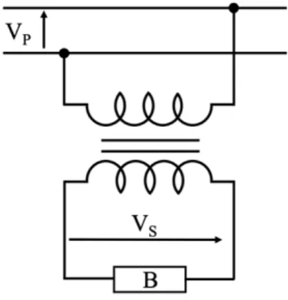
The capacitive-type voltage transformer (CVT) is basically a VT not directly connected to the power line. In between a series of two capacitors (𝐶W and 𝐶G) is installed; in particular, the VT is connected to the 𝐶G terminals (as depicted in Fig. 1.9), whereas the power line voltage is applied to the series of the two capacitors. This way it is possible to reduce extra-high voltages guaranteeing the safety properties of a standard VT.
Fig. 1.9. Schematic of a capacitive voltage transformer
1.1.3.3 Voltage transformers accuracy
As it is standardized in [5] for CTs, the accuracy parameters, ratio error and phase displacement, of a VT are defined in IEC 61869-3 [7]. They are defined as:
𝜀 =`ax*bx)
x) ∗ 100, (1.15)
∆𝜑 = 𝑈z&− 𝑈z", (1.16)
where 𝑈" and 𝑈& are the primary and secondary rms voltage of the VT under test, whereas 𝑘g is its
nominal ratio. In (1.16) the circumflexed quantities 𝑈z" and 𝑈z& refer to the phase of the primary and
secondary voltages.
Based on this, it is clear how the performance scenario of the inductive ITs has been well uniformized by International Standards. As a matter of fact, both kinds of ITs (including the unconventional ones, as described in the following chapters) are assessed by always referring to the same expressions. 1.1.4 Combined Transformers
An instrument that includes the features of VTs and CTs is the combined transformer. By definition, it is an “instrument transformer consisting of a current and a voltage transformer in the same enclosure” [1], hence it does not introduce novelties from a technological point of view but only in the application of different technologies. It is largely adopted in High Voltage (HV) primary stations, but it can be found even in Medium Voltage (MV) applications. They are typically installed in places with limited free space, as fewer mechanical structures are needed. In addition, the cost of combined transformers is lower than for single transformers. Fig. 1.10 includes a picture (left) and a simple schematic diagram (right) of the combined transformer.
Fig. 1.10. Picture (left) and simple schematic (right) of a combined transformer
The upper part of the transformer is dedicated to the primary terminals; in fact, the voltage is applied on just one of the current terminals. The main central part of the instrument provides the main connections for the two measured quantities: there is proper physical separation between the voltage and the current. This is also the main drawback of the combined solution: the two parts are separately insulated and contained inside the external insulation. Therefore, parasitic capacitances arise and are subjected to an electric field distributed in the height of the combined transformer. Finally, the lower part of the transformer contains the secondary voltage and current terminals, including the ground connection.
For the accuracy of the combined transformer, refer to Standard IEC 61869-4 [8]. In particular, the Standard assesses the transformer accuracy by using the ratio error and phase displacement expressions defined singularly for VTs and CTs.
1.2 Low-Power Instrument Transformers 1.2.1 Introduction
A new generation of ITs has been developed and spread in the last few decades. Initially, they have been referred to as non-conventional ITs; while after their standardization, they are referred to as Low-Power Instrument Transformers (LPITs) or simply “sensors” as another accepted term. The general aspects of LPITs are regulated by Standard IEC 61869-6 [9], defining these devices as: “arrangement, consisting of one or more current or voltage transformer(s) which may be connected to transmitting systems and secondary converters, all intended to transmit a low- power analogue or digital output signal to measuring instruments, meters and protective or control devices or similar apparatus”. In addition to this definition, it is essential to clarify the meaning of “low-power”. The Standard [9] states that an IT can be considered low-power if its output is typically lower than 1 VA. So, it is clear that the Standard has not been strict in defining the LPITs; therefore, the classification of ITs is not as straightforward as it seems, there is some degree of freedom to the manufacturer and user of such devices.
The LPITs structure, is shown in Fig. 1.11 in the block diagram, where the upper block-chain describes the general components of a passive LPIT, while the bottom blocks only apply to active LPITs. However, the block diagram, defined in [9], does not constitute a fixed schematic to build a LPIT but a general one which could vary depending on the considered device.
Fig. 1.11. General block diagram of a single-phase LPIT
Fig. 1.11 highlights that the basic principle of the LPITs is not common to all of them, but it varies depending on each technology for manufacturing them. The following section discusses two kinds of LPITs in detail, these are examined in the core of this thesis; the typical technologies adopted for LPITs are: resistive, capacitive, and resistive/capacitive dividers for Low-Power Voltage Transformers (LPVTs); and Rogowski coils, inductive transformers, shunts, for the Low-Power Current Transformers (LPCTs).
1.2.1.1 LPITs accuracy
The accuracy of the LPITs is just an extension of the concepts for the accuracy of inductive ITs. In fact, the definitions of ratio error 𝜀 and phase displacement ∆𝜑 still apply:
𝜀 =`a{*bj)
j) ∗ 100, (1.17)
∆𝜑 = 𝑌}&− 𝑋}". (1.18)
The differences rely only on the notation of the expressions; in fact, for the LPITs it is not always true that the input quantity is the same as the output one. Hence, there is a new notation in (1.17) and (1.18): 𝑋" and 𝑌& are the primary and secondary quantities, respectively; whereas 𝑋}" and 𝑌}& are the phases related to these quantities.
1.2.2 Current Transformers: Rogowski Coils
1.2.2.1 Basic principles
The Rogowski coil [10, 11] is a measurement device used to measure alternating currents. It consists of an iron-free toroidal core, typically made of air or other insulating materials, on which a solenoid is wound. Then, the conductor carrying the current to be measured is inserted in the Rogowski as shown in Fig. 1.12; where S and R are cross-section and radius, respectively.
at the solenoidal terminals, proportional to the mutual inductance 𝑀 between the primary and secondary conductors. Such phenomenon can be expressed as:
𝑢J(𝑡) = −𝑀‚K)(ƒ)
‚ƒ . (1.19)
Equation (1.19) shows that the Rogowski output is not a current proportional to the primary one, but a voltage proportional to the derivative of 𝑖"(𝑡). Therefore, in its basic configuration, the device
cannot provide a current-to-current relation to be used to process the measurement performed with the Rogowski coil. To obtain such a relation, an integrating block is necessary in cascade to the device; however, for the sake of simplicity and to avoid any external components, typical off-the-shelf Rogowski coils do not include any integrator. In addition, the coils are provided to the end users with a current to voltage ratio (e.g. 10 A/ 100 mV) to be used during measurements.
Based on these principles, it is possible to obtain an equivalent circuit of the Rogowski coil, valid for low frequencies including the power frequencies, 50 and 60 Hz. See Fig. 1.13, which contains:
• An ideal transformer, which provides the nominal ratio of the device; • an inductor 𝐿&: 𝐿&= …T -U‚ † G‡ log ‹ q, (1.20) • a resistor 𝑅&: 𝑅& = 𝜌 •Ž ‡gU, (1.21)
• a coupling capacitor 𝐶&,
𝐶& =•‡
U• T(‹Nq)
‘’“”moo•o , (1.22)
where 𝜌, 𝜀/, and 𝜇/ are the wire electrical resistivity, vacuum permittivity and permeability,
respectively. As for the geometrical parameters, N is the number of turns, b and a are the outer and inner diameters of the toroid, r is the wire radius, 𝑑P is the single loop diameter and 𝑙˜ is the length of the coil. For the sake of clarity, the meaning of the geometrical parameters is clarified in Fig. 1.14.
Fig. 1.14. Geometrical parameters clarification picture
Considering expressions (1.20) to (1.22) note that precise manufacturing information is required to obtain the Rogowski parameters; hence, obtaining such parameters is not straightforward for off-the-shelf devices.
1.2.2.2 Advantages and disadvantages
The previous subsection showed that the structure and the working principle of a Rogowski coil is quite simple. In addition, it has some features which can be compared briefly to legacy ITs.
The first feature derives from the core material, being iron-free, the Rogowski coil does not suffer from the nonlinearities of a typical IT; therefore, the Rogowski coil can be considered linear in its entire working range. Such a range is theoretically infinite, and significantly higher than the one of an IT, which is typically in the order of 10 times the rated current. Continuing with the geometrical features, a Rogowski coil is far smaller and more compact than an IT; hence it fits in all applications which do not have sufficient space for post-installation of instrumentation.
These coils also offer advantages regarding the measurements provided.: they work in a wide range of frequencies (from fractions of Hz to almost GHz) and they provide accurate answers to short transient input signals. In terms of safety, they guarantee the electrical insulation between the primary and the secondary circuits, considering that no active parts of the primary circuit are connected to the secondary windings.
However, Rogowski coils also have some drawbacks which make them unsuitable for certain applications. For example, the need of an integrating circuit in addition to the Rogowski coil makes it necessary to have power supply close to the Rogowski application, and that is not always possible for physical or safety reasons. Furthermore, Rogowski coils are very sensitive to the physical and electrical environment (i.e. primary conductor position, electric fields, temperature, etc.); hence a preliminary study on the location of the Rogowski coil is necessary to avoid collecting invalid measurements.
1.2.3 Voltage Transformers: Capacitive Dividers
1.2.3.1 Basic principles
Among the LPVTs, regulated by the IEC 61869-11 [12], the Capacitive Divider (CD) [13, 14] is one of the most common types. It is a passive LPVT and does not require any external power supply, which results in huge flexibility for in-field installation. As the name indicates, the CD consists of a series of two capacitors 𝐶 and 𝐶 as in Fig. 1.15; where 𝑉 and 𝑉
Fig. 1.15. Capacitive divider schematic
When the voltage 𝑉" is applied, the two capacitors are subjected to the same charge 𝑄 but not to the same voltage. The relationship between the charge and the capacitor value 𝐶 is described by the relation 𝑉 = 𝑄/𝐶. Hence, the higher the value 𝐶, the lower the voltage at its terminals. Therefore, the input/output expression of the CD is summarized by:
𝑉& = 𝑉" 5›
5›N5U (1.23)
In other words, to reduce the input voltage it is sufficient to have two capacitors with 𝐶W<𝐶G.
Such a simple technology is spread, in alternating current applications, along all voltage levels, from the low to the extra-high voltage. Fig. 1.16 shows two CDs, one for medium voltage (left), and one for high voltage (right). Note that in many CDs one of the capacitors is obtained directly using the insulating material which establishes the cage of the overall CD. In fact, the key point is to reach the desired value of capacitance, hence several technologies like the one mentioned are adopted by manufacturers.
Fig. 1.16. Picture of a medium voltage (left) and a high voltage (right) CD
1.2.3.2 Advantages and disadvantages
The widespread deployment of CDs is sustained by their numerous advantages with respect to other technologies. For example, compared to a resistive divider, a CD does not suffer from the heat dissipation due to the resistors. Hence, the current flowing through the divider is a not a limiting parameter of a CD. In terms of frequency, the CD is not subjected to any variation in its behavior because, even if the reactance is equal to 𝑋5 = G‡œ5W , the frequency dependency affects both the
application, due to the nature of their capacitors. Second, as defined in 1.2.3.1 and concluded in (1.23) these properties are true when ideal (or highly accurate) capacitors are considered. In fact, a real capacitor can be represented as the series of a capacitor and a resistor 𝑅P (also known as equivalent series resistor). The presence of the resistor gives rise to a series of side effects like the voltage drops and the dissipating heat, which can compromise the use of the capacitor and then of the application. To avoid such situations, a parameter used to quantify the capacitor “goodness” is the loss tangent 𝑡𝑎𝑛𝛿, defined as the ratio between the equivalent resistance of the capacitor and the reactance of the capacitor itself:
𝑡𝑎𝑛𝛿 = i†
jO . (1.24)
The angle 𝛿 expresses the amount of nonideality from theoretically 90° between the capacitor’s voltage and current phasors angles.
Therefore, extending the description of a single capacitor to the capacitive divider in Fig. 1.15, the following Fig. 1.17 shows the real capacitator. Hence, (1.23) turns into:
𝑉& = 𝑉"žž›
›NžU (1.25)
where 𝑍W= 𝑅W+ 𝑗𝑋5W and 𝑍G= 𝑅G+ 𝑗𝑋5G. Highlighting 𝑡𝑎𝑛𝛿, its effect on the final ratio of the divider can be assessed:
𝑉& = 𝑉" iUN jOU i›N jO›NiUN jOU= jOU(ƒqL¡UN ) jO›(ƒqL¡›N )NjOU(ƒqL¡UN ) = 5›(ƒqL¡UN ) 5U(ƒqL¡›N )N5›(ƒqL¡UN ) (1.26) In conclusion, the higher the 𝑡𝑎𝑛𝛿 of the adopted capacitors, the higher the discrepancy between the nominal and the actual ratio of the capacitive divider.
Chapter 2
INTERNATIONAL STANDARDS
After the description of ITs, it is fundamental to complete their overview from the Standard perspective. The regulation of ITs started more than two decades ago and evolved over the years. In 1996, the first documents of Standard IEC 60044-1 were published, followed by the remaining ones (60044-2 to 8) in the next years. They contained the definitions, test criteria and specifications for all typical transformers. At the end of the first decade of the 2000s, a new Standard series has been studied and developed by the Technical Committee 38 (TC 38) of the IEC with the aim of replacing the old series. This Standard is IEC 61869, from 1 to 15. The following section briefly examines these Standards to understand what is regulated and what is not for the different types of instrument transformers. In particular, only the Standards related to the ITs described in the previous chapter are studied.
To complete the survey of the Standards, consider EN 50160 [15] when dealing with ITs. The Standard contains the voltage characteristics for the electricity supplied on all voltage levels of the power networks (i.e. from low to high voltage); hence, it describes quantities that ITs are built to measure.
2.1 IEC 61869
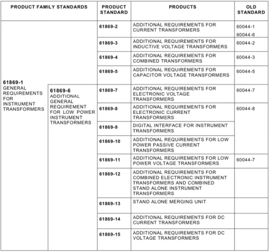
The Standard series is composed of 15 documents, each of which deals with a particular technology of instrument transformer or a general perspective on a group of them. To clarify this aspect, Fig. 2.1 lists a summary of the relevant documents along with the old Standards that they replace.
The picture shows that 61869-1 and -6 provide general requirements on instrument transformers and low-power instrument transformers, respectively, whereas the other Standards detail the requirements for specific kinds of transformers.
2.1.1 IEC 61869-1 and 61869-6
All Standards of the 61869 series share a common structure which helps the reader to navigate through the documents. In particular, 61869-1 and [16, 9], representing “general requirements” Standards, have been structured in the same way:
• A first part is dedicated to terms and definitions that holds for the entire document; usually citing other Standards and references.
• A second part contains the operating conditions of the device which the standard is referring to. The conditions are either normal or for special services.
• A third part defines the rated conditions for the related tests.
• A fourth part briefly contains the design and constructions requirements. In it, both the electromagnetic and mechanical requirements can be found.
• A fifth and last part is more useful for users testing the devices. In fact, the last part contains a detailed description and relevant thresholds for the tests to be carried out on instrument transformers.
In addition to the presented structure, the documents of the Standard share the definitions and statements included in them. It is suggested to browse both Standards to gain complete knowledge of the topics. The following subsections collect important aspects from both documents.
2.1.1.1 Operating conditions and rated values
The environment conditions are vital information for many types of devices. For ITs, IEC 61869-1 defines three temperature categories, listed in Table 2.1, which refer to the air temperature affecting the IT.
Table 2.1. Temperature categories for Instrument Transformers
Category Minimum Temperature [°C] Maximum Temperature [°C]
-5/40 -5 40
-25/40 -25 40
-40/40 -40 40
In addition to those limits, the Standard allows to extend them to -50 °C and +50 °C if the instruments are installed in very cold or very hot places, respectively. Humidity is another essential environmental quantity, and 61869-1 simply specifies that it must not exceed 95 % in a measurement window of 24 h. For the purpose of this thesis, temperature and humidity are the most significant quantities having stricter limits defined by the Standard. However, it defines other environmental quantities such as altitude, vibrations, and pressure.
As for rated values, Standard 61869-1, a general document, only defines them for quantities valid for all kinds of ITs. This includes the highest voltage applicable, the possible insulation levels, and the usable frequency.
In Standard 61869-6, describing low-power instrument transformers, the list of rated values is increasing. In particular, it defines two specific quantities: the level of the voltage supply, needed by an active LPIT, and the burden connected to it during tests. This is an impedance composed by a 2 MΩ resistor in parallel with a 50 pF capacitance. In addition, the Standard adds limits to the rated frequency 𝑓:
2.1.1.2 Tests on the ITs
Even for testing, both documents are coherent about their description. Standard 61869-1 defines four categories of tests:
• Routine test. Performed on each individual device to reveal possible manufacturing defects. • Type test. Performed only on a limited sample of each product to reveal issues not considered
in the routine tests.
• Special test. Specific tests defined in an agreement between customer and designer.
• Sample test. Special tests performed on one or more devices on particular aspects considered significant.
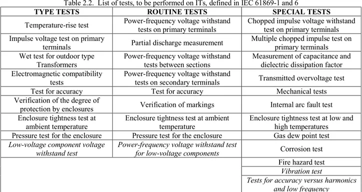
Such tests, listed in Table 2.2, are covered in all documents of the 61869 series. In particular, 61869-6 adds certain specific tests developed for the LPITs, and they are emphasized in italic in Table 2.2. Sample Tests, however, are not described in this table or in the Standards, because they are only developed when such requirements are established.
Table 2.2. List of tests, to be performed on ITs, defined in IEC 61869-1 and 6
TYPE TESTS ROUTINE TESTS SPECIAL TESTS
Temperature-rise test Power-frequency voltage withstand tests on primary terminals Chopped impulse voltage withstand test on primary terminals Impulse voltage test on primary
terminals Partial discharge measurement
Multiple chopped impulse test on primary terminals Wet test for outdoor type
Transformers Power-frequency voltage withstand tests between sections Measurement of capacitance and dielectric dissipation factor Electromagnetic compatibility
tests Power-frequency voltage withstand tests on secondary terminals Transmitted overvoltage test
Test for accuracy Test for accuracy Mechanical tests
Verification of the degree of
protection by enclosures Verification of markings Internal arc fault test
Enclosure tightness test at ambient temperature
Enclosure tightness test at ambient temperature
Enclosure tightness test at low and high temperatures
Pressure test for the enclosure Pressure test for the enclosure Gas dew point test
Low-voltage component voltage
withstand test Power-frequency voltage withstand test for low-voltage components Corrosion test Fire hazard test
Vibration test
Tests for accuracy versus harmonics and low frequency
The table shows that Standards already provide a quite complete set of tests to verify the performance of the ITs. In addition, for several tests, they provide the test setup and the configuration of the ITs to help the user performing the required tests. However, considering the technology evolution and the development of power networks in recent years, new tests arise day-by-day. For evident reasons, Standards cannot be updated so frequently; hence, the industry and academic research are expected to provide contributions to the testing process. In the core of this research activity, the main tests (and the new developed ones) mainly focus on accuracy, electromagnetic compatibility and temperature.
2.1.2 IEC 61869-2 and 61869-3
Standards 2 and 3 [5, 7] deal with “Additional requirements for inductive voltage transformers” and “Additional requirements for inductive current transformers”, respectively. According to the structure of the documents for the 61869 Standard, this subsection focuses on significant definitions and thresholds valid for inductive voltage and current transformers used in this thesis.
Table 2.3 collects those quantities, distinguished by the Standard from which they are taken. The output value and the burden are typically used to check if the device under test is aligned with the standard. As for the burden, it is essential to provide the correct value before starting the tests. The accuracy classes are divided by levels of accuracy: the letter S, which follows the class (e.g. 0.5S)
means that the guaranteed accuracy of the IT is higher than a 0.5 class one. Other significant quantities are the primary and secondary currents/voltages: the Standard defines several values for the current transformers, while it refers to another Standard, the IEC 60038 [17] for voltage. In addition, the table provides the voltage values referred to phase-to-phase measurements in a three-phase condition. Such values have to be divided by √3 if a single-phase measurement performed.
Table 2.3. Rated quantities defined in the Standards for inductive current and voltage transformers
Rated Quantity IEC 61869-2 IEC 61869-3 Output 2.5, 5, 10, 15, 30 VA 1, 2.5, 5, 10 VA
Burden 0.5, 1, 2, 5 Ω -
Accuracy Class 0.1, 0.2, 0.2S, 0.5, 0.5S, 1, 3, 5 0.1, 0.2, 0.5, 1, 3
Primary Current/Voltage 10, 12.5, 15, 20, 25, 30, 40, 50, 60, 75 A see IEC 60038
Secondary Current/Voltage 1, 5 A Typically 100, 200 V
The description of the accuracy class requires further detailing due to its role in this thesis. In fact, the measurement accuracy is one of the backbones of the thesis, examined in the following chapters. The accuracy class limits defined in [5, 6] are listed in Tables 2.4 and 2.5, respectively.
Table 2.4. Limits of the ratio error and phase displacement for inductive current transformers
Acc. Class
Ratio Error ±% Phase Displacement
At current (% of rated) At current (% of rated) ±Minutes At current (% of rated) ±Centiradians
5 20 100 120 5 20 100 120 5 20 100 120 0.1 0.4 0.2 0.1 0.1 15 8 5 5 0.45 0.24 0.15 0.15 0.2 0.75 0.35 0.2 0.2 30 15 10 10 0.45 0.24 0.15 0.15 0.2S 0.75 0.35 0.2 0.2 30 15 10 10 0.45 0.24 0.15 0.15 0.5 1.5 0.75 0.5 0.5 90 45 30 30 2.7 1.35 0.9 0.9 0.5S 1.5 0.75 0.5 0.5 90 45 30 30 2.7 1.35 0.9 0.9 1 3.0 1.5 1.0 1.0 180 90 60 60 5.4 2.7 1.8 1.8
Table 2.5. Limits of the ratio error and phase displacement for inductive voltage transformers
Acc. Class Ratio Error ±% ±Minutes Phase Displacement ±Centiradians
0.1 0.1 5 0.15
0.2 0.2 10 0.3
0.5 0.5 20 0.6
1 1.0 40 1.2
3 3.0 Not Specified Not Specified
The data in Tables 2.4 and 2.5 holds for the measurement purpose ITs. In fact, the Standards distinguish the measurement ITs from the protective transformers. This thesis discusses measurement ITs only; however, for the sake of completeness, the following section briefly explains definitions related to protective ITs. In addition, there are accuracy tables for all transformers covered here. Starting with the definition, a protective transformer is “a current transformer intended to transmit an information signal to protective and control devices” [5]. Such transformers can be identified by letters added to their accuracy class (e.g. P, PR, etc.). These new classes are defined as:
• Class P
“protective current transformer without remanent flux limit, for which the saturation behavior in the case of a symmetrical short-circuit is specified”.
“protective current transformer of low-leakage reactance without remanent flux limit for which knowledge of the excitation characteristic and of the secondary winding resistance, secondary burden resistance and turns ratio, is sufficient to assess its performance in relation to the protective relay system with which it is to be used”.
• Class PXR
“protective current transformer with remanent flux limit for which knowledge of the excitation characteristic and of the secondary winding resistance, secondary burden resistance and turns ratio, is sufficient to assess its performance in relation to the protective relay system with which it is to be used”.
• Class TPX
“protective current transformer without remanent flux limit, for which the saturation behavior in case of a transient short-circuit current is specified by the peak value of the instantaneous error”.
• Class TPY
“protective current transformer with remanent flux limit, for which the saturation behavior in case of a transient short-circuit current is specified by the peak value of the instantaneous error”.
• Class TPZ
“protective current transformer with a specified secondary time-constant, for which the saturation behavior in case of a transient short-circuit current is specified by the peak value of the alternating error component” [5].
These definitions all refer to current transformers, because the Standard introduces the protective instrument transformers in [5] and then only uses the information of Class P for VTs in [6].
For protective CTs, a new quantity has to be defined, the composite error: 𝜀5 = § › S∫ ©`aKªbK«¬ U ‚ƒ S T ,) 𝑥100 %, (2.1)
where 𝑖¯ and 𝑖J are the instantaneous values of the primary and secondary current, respectively. As for T, it represents the duration of one cycle, whereas 𝑘g and 𝐼" are the rated transformation ratio and the primary current rms value, respectively.
It is helpful to study the tables provided in [5, 6] for the accuracy specifications of the protective CTs and VTs (Table 2.6 and Table 2.7, respectively).
Table 2.6. Limits of the ratio error and phase displacement for protective inductive current transformers Acc. Class Ratio Error at rate current ±% Phase Displacement 𝜺 𝑪 at rated current % Minutes Centiradians 5P and 5PR 1 ±60 1.8 5 10P and 10PR 3 - - 10 TPX 0.5 ±30 ±0.9 - TPY 1.0 ±60 ±1.8 - TPZ 1.0 180±18 5.3±0.6 -
Table 2.7. Limits of the ratio error and phase displacement for protective inductive voltage transformers
Acc. Class Ratio Error ±% ±Minutes Phase Displacement ±Centiradians
3P 3.0 120 3.5
2.1.3 IEC 61869-4 and 61869-12
The Standards 61869-4 and 12 [8, 18] deal with the combined (voltage and current) inductive transformers and the low-power version, respectively. As for document 12, it is still under development by the technical committee, so this thesis can only evaluate Standard 61869-4.
The document contains “Additional requirements for combined transformers”, which means “an instrument transformer consisting of a current and a voltage transformer in the same case” [1]. In this document, take particular note of the tests related to the combined presence of voltage and current sensors, aside from the other points in common with the other Standards. Such a set of tests has been developed to assess the performance of the IT in presence of this particular feature, and it can be briefly summarized below:
• First, the voltage ratio error and the phase displacement are determined with no current supplied to the IT (according to [7]).
• Second, the current is then applied to the IT and the accuracy parameters determined one more time.
The same procedure, substituting the voltage with the current, is applied to test the influence of the voltage transformer on the current one. Moreover, in the Standard, an annex is completely dedicated to further explain this physical phenomenon (not included in this thesis).
2.1.4 IEC 61869-10 and 61869-11
IEC 61869-10 and 11 [19, 11] provide “Additional requirements for low-power passive current transformers” and “Additional requirements for low-power passive voltage transformers”, respectively. They follow the structure used for documents 2 and 3 of the series; however, they cover the new LPIT (or sensors).
The rated values defined in [5] and [7] also apply to the LPITs with only minor changes when necessary; for instance, the new sensors have transmitting cables not included in inductive transformers. Primary and secondary values are different and are collected in Table 2.8.
Table 2.8. Rated quantities defined in the Standards for low-power current and voltage transformers
Rated Quantity IEC 61869-10 IEC 61869-11 Primary Current/Voltage 5, 10, 20, 50, 100 A See IEC 60038
Secondary Current/Voltage 22.5, 150, 225 mV 3.25/√3, 100/√3 V
Conversely, the accuracy thresholds and specifications have been modified to include the new features of these devices. In particular, the values of Table 2.5 are still valid for the voltage sensors, except for the protective ones which limits are listed in Table 2.9.
Table 2.9. Limits of the ratio error and phase displacement for protective LPVTs
Acc. Class
Ratio Error ±% Phase Displacement
At voltage (% of rated) At voltage (% of rated) At voltage (% of rated) ±Minutes ±Centiradians
2 20 80 100 2 20 80 100 2 20 80 100 0.1P 0.5 0.2 0.1 0.1 20 10 5 5 0.6 0.3 0.15 0.15 0.2P 1 0.4 0.2 0.2 40 20 10 10 1.2 0.6 0.3 0.3 0.5P 2 1 0.5 0.5 80 40 20 20 2.4 1.2 0.6 0.6 1P 4 2 1 1 160 80 40 40 4.8 2.4 1.2 1.2 3P 6 3 3 3 240 120 120 120 7 3.5 3.5 3.5 6P 12 6 6 6 480 240 240 240 14 7 7 7
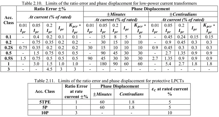
Table 2.10. Limits of the ratio error and phase displacement for low-power current transformers
Acc. Class
Ratio Error ±% Phase Displacement
At current (% of rated) At current (% of rated) ±Minutes At current (% of rated) ±Centiradians
0.01 𝑰𝒑𝒓 0.05 𝑰𝒑𝒓 0.2 𝑰𝒑𝒓 𝑰𝒑𝒓 𝑲𝒑𝒄𝒓∗ 𝑰𝒑𝒓 0.01 𝑰𝒑𝒓 0.05 𝑰𝒑𝒓 0.2 𝑰𝒑𝒓 𝑰𝒑𝒓 𝑲𝒑𝒄𝒓∗ 𝑰𝒑𝒓 0.01 𝑰𝒑𝒓 0.05 𝑰𝒑𝒓 0.2 𝑰𝒑𝒓 𝑰𝒑𝒓 𝑲𝒑𝒄𝒓∗ 𝑰𝒑𝒓 0.1 - 0.4 0.2 0.1 0.1 - 15 8 5 5 - 0.45 0.24 0.15 0.15 0.2 - 0.75 0.35 0.2 0.2 - 30 15 10 10 - 0.9 0.45 0.3 0.3 0.2S 0.75 0.35 0.2 0.2 0.2 30 15 10 10 10 0.9 0.45 0.3 0.3 0.3 0.5 - 1.5 0.75 0.5 0.5 - 90 45 30 30 - 2.7 1.35 0.9 0.9 0.5S 1.5 0.75 0.5 0.5 0.5 90 45 30 30 30 2.7 1.35 0.9 0.9 0.9 1 - 3.0 1.5 1.0 1.0 - 180 90 60 60 - 5.4 2.7 1.8 1.8 3 - - 4.5 3 3 - - - - Table 2.11. Limits of the ratio error and phase displacement for protective LPCTs
Acc. Class Ratio Error at rate current ±% Phase Displacement 𝜺 𝑪 at rated current % ±Minutes Centiradians 5TPE 1 60 1.8 5 5P 1 60 1.8 5 10P 3 - - 10
Note that Table 2.11 has defined a new class for protective LPCT: the TPE. “Class TPE low-power current transformers are designed for relay protection applications. The accuracy is defined by the highest permissible percentage composite error at the rated accuracy limit primary current prescribed for the accuracy class concerned. Class TPE designates transient protection electronic class CTs. Class TPE is defined by a maximum peak instantaneous error of 10 % at the accuracy limit condition, the rated primary circuit time constant, and the rated duty cycle. The peak instantaneous error includes direct and alternate current components. This is equivalent to the definition of TPY-class CTs” [9]. Comparing Tables 2.4 and 2.10, it can be concluded that the values at the rated current coincide, while Table 2.11 provides an extended set of accuracy limits for additional accuracy classes. Finally, the tables show the accuracy classes corresponding to the primary currents selected.
The tests described in IEC 61869-10 and 11, are examined in Chapter 4. 2.2 EN 50160
The Standard EN 50160 is entitled “Voltage characteristics of electricity supplied by public electricity networks”. In 2010, the latest version has been published superseding the 2007 one. The document has an easy-to-read structure which includes, aside from basic terms and definitions, three main chapters dedicated to low, medium, and high voltage supply characteristics. This thesis does not discuss high voltage characteristics, but focuses on medium and low voltages.
2.2.1 Medium and Low Voltage supply characteristics
Defining the characteristics of all voltage levels available in power networks, the Standard starts from the rated values of the main quantities and then describes the possible phenomena which can occur during normal operation of a network. Such descriptions contain the limits for the major quantities in all relevant working conditions.
By starting with standardized values, the nominal low and medium voltages are 230 V and between 1 kV and 36 kV, respectively. The frequency is the second and last reference quantity, it is the same for both voltage levels:
• for systems with synchronous connection to an interconnected system o 50 Hz ±1 %, during the 99.5 % of the year.
o 50 Hz +4 %, -6 % during the 100 % of the year.
o 50 Hz ±15 %, during the 100 % of the year.
These values show that the frequency limits are less strict for more delicate power networks with fewer connections.
The phenomena in voltage supply coincide for both low and medium voltages, and they are divided in two kinds of phenomena: continuous phenomena and voltage events. The former is a deviation from the nominal value that occurs continuously over time; the latter instead is a sudden and significant deviation from the nominal or desired wave shape. A complete list of phenomena and events is presented in Table 2.12.
Table 2.12. List of low/medium voltage phenomena and events
Continuous Phenomena Voltage Events
Supply voltage variations Interruptions of the supply voltage
Rapid voltage changes Supply voltage dips/swells
Supply voltage unbalance Transient overvoltages
Harmonic voltage Interharmonic voltage Mains signaling voltages
Note the mentioning of harmonics and interharmonics. These are highly important as a power quality issue of the grid, and will be discussed in the following chapters. Hence, according to the Standards the presence of harmonics in voltage supply is limited to the values in Table 2.13; while for interharmonics the Standards do not yet include any limits.
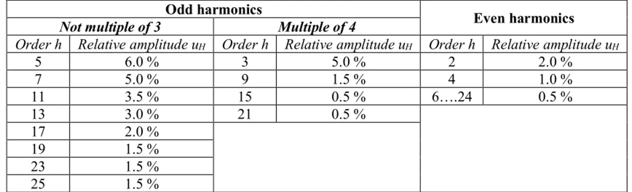
Table 2.13. Percentage of the maximum value of each single harmonic allowed over the voltage supply
Odd harmonics Even harmonics
Not multiple of 3 Multiple of 4
Order h Relative amplitude uH Order h Relative amplitude uH Order h Relative amplitude uH
5 6.0 % 3 5.0 % 2 2.0 % 7 5.0 % 9 1.5 % 4 1.0 % 11 3.5 % 15 0.5 % 6….24 0.5 % 13 3.0 % 21 0.5 % 17 2.0 % 19 1.5 % 23 1.5 % 25 1.5 %
The table shows that each harmonic order has a peculiar limit depending on the severity and importance of such harmonic for the power network. In addition, the Standard limits the list to the 25th harmonic, because the higher order ones have very low impact on the network and are quite
unpredictable.
In conclusion, the adoption of two Standards like the EN 50160 and the IEC 61869 series allows to have all necessary information when investigating ITs and how to test them. The Standards cover all existing kinds of ITs and the electricity they are supplied with, detailing the information required by the user before and after performing tests. However, the Standards do not include all possible tests, so they are subjected to periodical updates. Contributing to future updates of these regulatory documents, the main part of this thesis introduces new tests having the design based on these Standards.
Chapter 3
The Role of Uncertainty
This chapter introduces and discusses the role of metrology, the science of measurement, and the impact of uncertainty on the process and results of measurements. This includes essential principles and definitions that apply to scientific measurements in general, and an overview on basic and advanced aspects of uncertainty on metrology.
3.1 Basic Principles
What is Metrology? In [1], it is defined as “science of measurement and its application – it includes all theoretical and practical aspects of measurement, whatever the measurement uncertainty and field of application”. Consequently, measurements are the pillars of such a science, and they are defined, [1], as “process of experimentally obtaining one or more values that can reasonably be attributed to a quantity".
It is common to apply this process on a daily basis, consciously or unconsciously, to obtain information and data from the surrounding world, such as understanding how much space is left in a shopping bag by looking inside of it, or sending shuttles to space by using instrumentation worth billions of euros.
When applying such a process, it concerns a property that is subjected to the measurement: the quantity. It is defined in [1] as “property of a phenomenon, body, or substance, where the property has a magnitude that can be expressed by means of a number and a reference”. Note that the concept of quantity can be also extended to vectors or tensors, whose components are quantities as well. It is not possible to determine or obtain the "true value" of a quantity, instead a "reasonable" value for the measurand is estimated. The reasonable estimation in this definition indicates that the result of a measurement is not the true, actual value of the measurand; that value is unknown and it is only possible to estimate it.
So, the issue is the lack of knowledge about the real result of a measurement. This is known as uncertainty, and it is, [1], a “parameter, associated with the result of a measurement, that characterizes the dispersion of the values that could reasonably be attributed to the measurand”. So, uncertainty quantifies the level of lack of knowledge associated to a measurement, and there are three major types of the uncertainties [20]: definitional, interaction, and instrumental uncertainty.
The definitional uncertainty is directly related to the measurand, and it results from the imperfect definition of a measurand and its model. Before any measurement a preliminary model with various degrees of complexity is established, and this is never perfect.
The interaction uncertainty results from using a measurement instrument. When an instrument is connected to a measurand, the instrument is affecting and altering the quantity to be measured. The instrumental uncertainty is another aspect resulting from the instrumentation. The instrument performing a measurement introduces such uncertainty due to its intrinsic imperfection, even if it is based on a standard reference.
These types of uncertainty affect the final measurement results, which can be grouped in two main categories [20]: systematic and random effects. Systematic effects occur continuously, they are highly difficult to detect but also easy to correct and remove if encountered. Random effects, on the other hand, are fully arbitrary and unpredictable phenomena, which cannot be compensated for. However, their effect on final results can be almost completely removed by repeating the same type of measurement. In this case, the statistical expectation of the random error on repeated measurements is zero.
Consider these examples. A systematic effect can be seen as a constant weight affecting a scale while measuring. In the measurement, a small amount of weight is subtracted or added to whatever
measurand, leading to an invalid result. A typical example for a random effect is the noise superimposed on a measurand which cannot be predicted as it manifests itself in an arbitrary way. Fig. 3.1 provides a graphic representation of these effects. The “actual” signal is depicted in blue, while red and yellow colors indicate the signals affected by systematic and random effects, respectively.
Fig. 3.1. Example of signal affected by random (yellow) and systematic (red) effects
In a conclusion, note it is not possible to obtain the true value of a quantity by measuring. There is no measurement without uncertainty. To be clear, providing a measurement without its uncertainty renders such measurement as ineffective and meaningless.
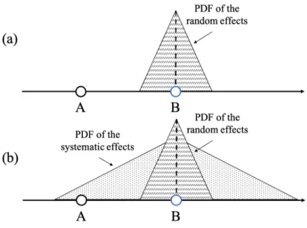
Note the particular aspects of the systematic error. As stated above, it is typically difficult to detect systematic errors, but what happens when it is not detectable at all or when the available information is not sufficient? An example is the error provided by the instrument’s manufacturer. It is typically the maximum value (positive) obtained from the series of instruments tested along with the one that is being used. During a measurement, this results in shifting of possible “true” value (A) to a new attributed value (B), as depicted in Fig. 3.2. Therefore, even if multiple measurements are performed, the result will be wrongly centered in a position different from the “true” value (case (a) Fig. 3.2). An adopted solution is the application of a probabilistic approach to treat the systematic errors. This way, both the random and the systematic effects are treated as a probability density function (PDF), which together compose the overall uncertainty (case (b) Fig. 3.2). One way to combine both effects in a PDF is by applying the Monte Carlo method, briefly described in 3.2.2.3.
Fig. 3.2. Example of how to treat unknown systematic effects
3.2 Guide to the Expression of Uncertainty in Measurements 3.2.1 Introduction
The guide to the expression of uncertainty in measurements (GUM) [21] and its related documents [22, 23] have been developed by the Joint Committee for Guides in Metrology (JCGM) with a specific purpose: to spread the evaluation of measurement uncertainty by using the guidelines provided in the documents. These are aimed at helping experts, either in industry or in academia, increasing the role of uncertainty evaluation in their fields and research topics. Such documents,consist also of a useful tool for operators and non-experts with instructions how to process measurement results, and how to present them to an audience. Conversely, the GUM series may not be easy to comprehend for people with limited educational background. Therefore, experts are continuously trying to enhance the documents, including specific application examples extrapolated from the GUM.
The next subsection provides a general overview of the GUM core, to obtain multiple results: introducing and refreshing the concept of uncertainty evaluation, and clarifying some aspects useful in the later sections of the thesis.
3.2.2 The GUM
Following the introduction in the previous sections, it is fundamental to obtain a quantity that reflects the quality of a given measurement result. This should be done applying a universal method in order to compare measurements results either among a series of them or among results obtained from different Standards or datasheets. This quantity is the uncertainty, which is substituting the legacy error analysis, and as described in the following it is expressed as a coverage probability or level of confidence. This last parameter is defined as “the value (1 − α) of the probability associated with a confidence interval or a statistical coverage interval”, [21].
3.2.2.1 Basic definitions and concepts
Before discussing the uncertainty evaluation, it is essential to define some basic concepts:
• Standard uncertainty: uncertainty of the results of a measurement expressed as a standard deviation.
• Type A evaluation of uncertainty: method of evaluation of uncertainty by the statistical analysis of series of observations.