Analysis and preliminary realization of a brake pad contact detection system

1

POLITECNICO DI MILANO

Scuola di Ingegneria Industriale e dell’Informazione

Corso di Laurea Magistrale in Ingegneria Elettrica

ANALYSIS AND PRELIMINARY REALIZATION

OF A BRAKE PAD CONTACT DETECTION

SYSTEM

Relatore: Professore Francesco Castelli Dezza

Correlatore : Professore Stefano - Melzi

Tesi di Laurea Magistrale di:

MATTIA FEDERICO LEVA

Matricola 858334

i

Contents

Introduction

1

Chapter 1

2

1 Electrical contact system 2

1.1 Electrical contact 2

1.2 Electrical contact surfaces 3

1.3 Contact resistance 4

1.4 Theoretical contact resistance evaluation through a-spots 5

1.5 Film resistance 8

1.6 Temperature influence 9

2 Mechanical brake system 10

2.1 How the braking system works 11

2.2 Friction theory 12

2.3Types of Friction Braking Systems 12

2.3.1 Drum Brakes

13

2.3.2 Disc Brakes

13

2.3.3 Disc brake components 14

2.4 Wear pad sensors 22

2.4.1 Squealer type 22

2.4.2 Resistive circuit type 23

2.4.3 Electronic parking motion type 24

Chapter 2

25

1.1 Electrical conductive characterization of mechanical components 25

2.1 Components characterization 26

3.1 Capacity test with frequency sweep 44

3.2 Incremental distance 53

3.3 Single pad analysis of the complete system 56

Chapter 3

59

ii

2.1 Simulation setup 59

2.2 Simulation configuration process 60

3.1 DC Conduction 62

3.2 Current density distribution 70

4.1 Electrostatic Simulations 75

4.2 Capacitance matrix 75

4.3 Simulation setup 78

4.4 Final impedance value 87

Chapter 4

88

4.1 AD5933 system description 89

4.2 Measurement setup 92

4.3 Advantages versus disadvantages 93

4.4 Experimental test on the EVAL-AD5933EB board 94

Conclusion

105

Bibliography References

106

iii

Abstract

Up to now, when thinking about advancing the efficiency of a vehicle, all the components under investigation are purely related to the engine, aerodynamics and tire compounds. The importance of the braking system is usually underestimated. In addition another element scarcely taken into account is the pollution produced by the brake pad components during braking. Braking system is a mechanical device, one of the most important elements for the right functioning of a vehicle. It inhibits motion by converting kinetic energy into heat or in the newest hybrid cars in electrical energy storable in batteries. The aim of this thesis is to identify the presence of unwanted contacts between brake disc and brake pads when braking is not requested by the driver. More precisely, a deep experimental analysis, is made on the electrical characterization of the brake pad studying it as one electrical element component, on the possible unwanted contacts configurations and the evaluation of these through an impedance variation. The solution proposed consists in comparing the measurements taken between a set of brake pads with a series of reference impedance values in order to obtain the relative distance between pad and disc. Three approaches have been adopted: the first one is an experimental one, the second one based on electronic simulations and the third one related to the production of an industrial product.

iv

Figure Index

Figure 1: Surface contact spots

Figure 2: Resistivity-Temperature trend Figure 3: Automotive braking system Figure 4: Drum brake components Figure 5: Fixed caliper

Figure 6: Floating caliper Figure 7: Brake disc comparison Figure 8: Brake pads typologies Figure 9: Squealer wear indicator

Figure 10: Resistance value of a cast iron ring Figure 11: 1:1 Scale brake pad

Figure 12: Four quarter of the brake pad during the 1/24 analysis Figure 13: First quarter impedance measurement

Figure 14: Scotch tape pre-cut stage Figure 15a: Outside 1cm border impedance Figure 15b: Inside 1cm border impedance Figure 16: Lateral extremes impedance Figure 17: Horizontal stripes

Figure 18: 8th order impedance characterization curve Figure 19: Connection clamps points

Figure 20: 4 pressure points versus 2 pressure points configuration Figure 21a: Pad right to the designated slot

Figure 21b: Pad above half right slot

v

Figure 21d: Pad above half left slot

Figure 21e: Pad left to the designated slot

Figure 22: Pads placed on same surface configuration

Figure 23: Capacitance measurement with pad position configuration

180°above and side to side bottom

Figure 24: simplified pad positioning (above) versus real pad positioning

(below)

Figure 25: Short-circuiting the right pad

Figure 26: Short-circuited equivalent circuit (left) compared to the complete

equivalent circuit (right)

Figure 27: DC conduction applied voltages

Figure 28: Complete pad-disc contact

Figure 29: Quarter pad-disc contact

Figure 30: Half quarter pad-disc contact

Figure 31: Current density distribution with total contact

Figure 32: Ratio between current density distribution over different contact

areas

Figure 33: Electrical equivalent system of the braking system

Figure 34: Region setup comparison

Figure 35: AD5933 board block diagram

Figure 36: System connections

Figure 37: Automotive system connections

Figure 38: Calibration setup of the EvalAD5933EBZ board

Figure 39: Software parameter for board calibration

Figure 40: Impedance measurement setup

vi

Table Index

Table 1: Relationship between a-spots shape and Resistance

Table 2: Relation between a-spot radius and resistance value

Table 3: Pie chart of pad materials

Table 4: Cast iron bulk resistivity

Table 5: Resistance values of the pad divided in 24 parts

Table 6: Four quadrant impedance

Table 7: Half quarter impedance vertical case

Table 8: Half quarter impedance horizontal case

Table 9: Border impedance

Table 10: Left-Right/Center impedance

Table 11: Horizontal section impedance

Table 12 (a, b, c, d, e, f, g): Resistance and Capacitance values over three main setup

Table 13: Quadrant area values

Table 14: Resistance values expressed in ohm of the over mentioned configurations

Table 15: Resistance times relative area values

Table 16: Parameters comparison

Table 17: Capacitance frequency sweep results

Table 18: Frequency sweep resistance-capacitance analysis in six different configurations

Table 19: Capacitance measurement with same surface and angle displacement

Table 20: Incremental distance comparison between the two configurations Table 21: Numerical results of short-circuiting one pad

vii

Table 23: Relation between pad contact cases and total loss

Table 24: Relation between pad contact cases and resistance

Table 25: Iterative process for conductivity value

Table 26: Final total loss and resistance values with definitive bulk conductivity

Table 27: Comparison between same surface and opposite surface capacitive behavior

Table 28: Long distance capacitance measurements

Table 29: Comparison between simulation and experimental results

Table 30: Peak to peak voltage of the output signal

viii

Graph Index

Graph 1: Four quadrant impedance

Graph 2: Case b and c impedance comparison

Graph 3: Total configurations impedance measurement comparison Graph 4: Resistance times area behavior

Graph 5: Same surface incremental distance capacitance Graph 6: Opposite surface incremental distance capacitance Graph 7: Comparison between graph 5 and 6

Graph 8: Relation between pad contact area and total loss Graph 9: Iterative conductivity identification process

Graph 10: Capacitive simulation trend at different percentage errors Graph 11: Same surface versus Opposite surface capacitive trend Graph 12: Simulation versus experimental tests

1

Introduction

This thesis deals with the possibility to improve and increase the global automotive efficiency by installing an electronic devices which measures the impedance of the wheel brake setup. The presented solution is one of the possible approaches to the problem and it aims to reduce unwanted contacts during ordinary driving, so increase vehicle efficiency in terms of eco-sustainability both in a reduction of fuel consumption, pads wear and fine dust particles emissions.

The analysis has been structured in four chapters

The first chapter is subdivided in two parts. The first one explains how electric contact works and how resistance can be measured depending on the environmental conditions. The second one, on the other hand, treats the mechanical features of the braking system of a vehicle. The focus is set especially on disc brake components and brake pad composition.

In the second chapter, an experimental approach has been opted for the braking system in order to evaluate the possibility to establish a closed electrical circuit and define the electro-mechanical characters. In particular the electrical ones are bulk conductivity, permittivity and impedance in terms of resistance and capacitance.

The third chapter exposes the results of the finite element method (FEM) simulations. In order to accomplish this task the software used are Ansys Electronics and Solidwork2016 for the system design. Two main different setup are considered: DC conduction for current density distribution and Electrostatic analysis for the capacitance matrix configuration.

The fourth chapter proposes a possible solution to the measurement problem, by the use of an evaluation board which allows to detect the presence of unwanted contacts. The solution is both explained in a theoretical way and through an experimental frequency sweep analysis.

2

Chapter 1

Electrical contact system

1.1 Electrical contact

An electrical contact is defined as the interface between the current-carrying members of electrical devices that assure the continuity of electric circuit. The current-carrying members in contact, often made of solids, are called contact members or contact parts, meanwhile the current-receiving ones can be both solids or liquids. The contact members connected to the respective positive and negative circuit clamps are called anode and cathode.

Electrical contacts provide electrical connection between parts and they perform many functions. The primary purpose of an electrical connection is to allow the uninterrupted passage of electrical current across the contact interface. The best possible connection can only be achieved when a metal-to-metal contact is established. Although the nature of the contact processes may differ from one to another, they are all governed by the same fundamental phenomena. The most important are degradation of the contacting interface and the associated changes in contact resistance, load, temperature, and other parameters of a multipoint contact.

Electrical contacts can be classified according to their nature, surface geometry, kinematics, design and technology features, current load, application, and by others means.

In general, electrical contacts can be divided into two basic categories: stationary and moving.

 Stationary contacts, contact members are connected rigidly or elastically to the stationary unit of a device to provide the permanent joint. They are divided into non-separable or all-metal (welded, soldered, and glued), and clamped (bolted, screwed, and wrapped). 1.Non-separable(permanent) joints have a high mechanical strength and provide the stable electrical contact with a low transition

3 resistance. A non-separable joint is often formed within one contact member.

2. Clamped contacts are made by mechanically joining conductors directly with bolts or screws or using intermediate parts called clamps. These contacts may be assembled or disassembled without damaging the joint integrity.

 Moving contacts are characterized by at least one rigid or elastic contact member connected to the moving unit of a device. Depending on their operating conditions, these contacts are divided into two categories: commutating and sliding.

1. Commutating contacts intermittently control the electric circuit. They fall into two categories: separable (various plug connectors, circuit breakers) and breaking.

2.In sliding contacts, the contacting parts of the conductors slide one over the other without separation. Current passage through the contact zone is followed by physical phenomena (electrical, electromechanical, and thermal) that produce changes on the surface layers of the contacting members. The severity of the processes occurring at contact interface depends on the magnitude and character of the current passing through the contact points, the applied voltage, operating conditions, and contact materials used .

1.2 Electrical contact surfaces

Ideal surfaces are completely flat and homogeneous in all its points. Real surfaces on the other hand are not uniform and plain but includes many asperities and defects.

Therefore, when contact is made between two surfaces, in our case between brake pads and brake disc, all the imperfections and asperities with maximum height of both members come into contact. Higher the braking load is

4 required, higher will be the amount of defects come in contact forming spots. The overall area of these spots is known as the real contact area. This area depends both on the mechanical behavior of the surface layers and their roughness. It is continuously changing and at each braking pressure applied it modifies itself. Once the braking is released the contact are should be zero, and an air gap is formed between contact surfaces. This process of contact and detachment can be seen as an electrical switch characterized by a varying impedance.

This process leads to the evaluation of the electrical impedance.

1.3Contact resistance

As mentioned before solid surfaces are always rough. The dimension of asperities and defects can vary from the length of the sample to the atomic scale. By convention, the surface irregularities are classified into errors in form, waviness, roughness, and sub-roughness (nano-scale roughness). Those levels of roughness are associated with corresponding types of contact area (apparent, real, and physical area of contact). Study of these areas follows the general trend of mechanics from the macroscopic models up to the current attempts to understand the micro/nano scale processes in the contact of solids. The surface topography affects all the contact characteristics but primarily the mechanical ones. Another important factor affecting the contact behavior is the presence of various films (such as oxides, contaminant dusts, reaction products and water) which interfere in the system.

The hypothetical electrical circuit evaluated should be an ensemble of mechanical components involving the automotive mechanical braking system. The “closing circuit component” is the connection of pads with the rotating disc.

5 The current passes through the “a-spots” that are smaller than the theoretical contact spots when braking is in course, meanwhile an open circuit is present when braking is not applied.

Since the electrical current lines are constricted to allow them to pass through the a-spots ,as shown in Figure (1), the electrical resistance increases. This increase is defined as the constriction resistance. Moreover if contaminant films are considered, on the mating surfaces an increase the resistance of a-spots is noticed. The total resistance due to constriction and contaminant films determines the contact resistance.

Figure 1: Surface contact spots

The fundamental monograph of Holm considered most of the contact phenomena important for mechanical and electrical aspects. Holm’s approach is focus on the description of the factors of either electrical or thermal origin affecting the contact resistance. In the case of isotropic roughness topographies, the a-spots are assumed to be circular or noncircular when the roughness has a directional characteristic (e.g., in rolled-metal sheets or extruded rods).

1.4 Theoretical contact resistance evaluation through a-spots

Lets start by considering two cylinders C1 and C2, defining their contact surfaces As1 As2 and their theoretical contact surface Aa. Due to the presence of imperfections and asperities of surfaces C1 and C2 the real contact surface is defined as Ac. The current flux flows from the cathode As1 to the anode As2 through Ac. This phenomena brings to what is called constriction resistance between two points, a and b, of the cylinders. It is evaluated as:

6

Considering one cylinder and assuming the total area Aa is made of perfectly conductive material, so that the current flux flows parallel to the cylinder, the ideal total contact resistance ) can be determined by applying a voltage potentials between a and b.

The constriction resistance and the applied voltage are defined as:

) In case of simple contact, without any type of film on the surface, R is simply defined as contact resistance. In case a film is present, for example iron oxide on disc rotor, the contact resistance R should be the sum of the constriction resistances of both conductors plus the film resistance

Where : “n” corresponds to the number of a- spots and “a” to their section. The film resistance for instance is expressed as:

(1.6)

Constriction resistance for a single a-spot between two conductors of semi infinite length is given by:

And considering both conductors it becomes:

7 Respectively the resistivity of the conductor ( ), and the conductor asperity diameter ( ).

If different materials have been used for the two conductors, such as the case we are going to study, it is possible to rewrite the above mentioned resistance as:

In more detail, construction resistance of one circular asperities with radius “a” of cylindrical conductor with radius R can be rated as the solution of the Laplace equation:

Constriction resistance is function of the number and the dimension and the shape of the a-spots. Supposing to have different a-spots shapes we can get different resistance values as it is reported in Table 1:

a-spot shape Radius [μm] Length [μm] Width [μm] Ring thickness [μm] Resistance [Ω] Circular 5.64 1.55*10^-3 Squared 10 10 3.04*10^-3 Rectangular 50 2 0.43*10^-3 Ring 16.41 1 0.71*10^-3

Table 1: Relationship between a-spots shape and Resistance

Once the a-spots are defined, in an electric contact the number of asperities depends from the braking force required, so by a mechanical load. It is

8 possible that some of these deformity get together forming a group called cluster. In this situation a new equation is labeled. Always taking into account the circular geometry of the a-spots it results:

The cluster radius is also called Holm radius and is indicated with a. In Table 2 are reported some interesting values regarding the above formula

progressively increasing the a-spots radius.

a-spot radius [μm]

a-spot resistance [Ω]

Holm radius (a) [μm] Cluster resistance [Ω] Single a-spot radius equivalent resistance [Ω] 0.02 0.3289 5.34 0.0937 1.18 0.04 0.1645 5.36 0.0932 1.94 0.1 0.0685 5.42 0.0923 3.16 0.2 0.0329 5.50 0.0909 4.04 0.5 0.0132 5.68 0.0880 4.94

Table 2: Relation between a-spot radius and resistance value

The real contact area depends on the mechanical applied load. The

deformation of the parts in contact can be of two types: plastic or elastic. The difference between the two consists in the contact pressure which follows the Hertz theory.

1.5 Film resistance

The film resistance takes into account of the contribute of the contact resistance due to the presence of contaminated layers on the contact surface. These films can be: oxidation layers, lubricants, water and corrosive agents

9 which due to their high resistivity tends to limited conduction and so the current flows.

Conduction is not prohibited, these layer are really thin , on average less than 10-10m, and can conduct thanks to the tunnel effect. In traditional mechanic energy conservation law states that a particle can’t overcome an obstacle if it doesn’t have to energy to do it. On the other hand quantum mechanics allows a probability, a really small one, to the particle to be able to overcome the barrier. Since it is a probability, the tunnel effect resistivity is independent to the film composition.

Calling ρf the contaminated layer resistivity, s the layer width and with Σa the summation of all the contaminated areas, resistance can be written as:

Hypothesizing an uniform distribution of the layer above the contact surface, meaning that Σa=A, it is possible to rewrite film resistance as:

where H is the hardness of the contaminant layer and F the applied load. The relationship between F and H is defined by the law:

1.6 Temperature influence

In the previous formula contact resistance has been found in relation with resistivity ρ of the material. Resistivity is function of temperature:

ρ0 is the resistivity at standard temperature, ρT the one at the desired temperature, T0 the reference temperature and α the temperature coefficient.

10 When temperature increases the vibrations of the metal ions in the lattice structure increases. These vibrations bring to collision between free electrons and the other electrons. Each collision scoops out a bit of energy from free electrons and causes electrons inability motion. This process reduces the movements of the delocalized electrons and drift velocity. As a consequence resistivity of the conductive material increases and current flow decreased. In the Figure (2) is depicted the behavior of resistivity as function of temperature for conductors

Figure 2: Resistivity-Temperature trend

Mechanical brake system

In order to slow or stop a vehicle the kinetic and any potential energy of the vehicle’s motion must be dissipated in heat or converted into electrical energy. Friction brakes operate by converting the energy of the vehicle’s motion into heat and dissipating it to the atmosphere. This process is an irreversible process that is nowadays is been reduced by hybrid and full

11 electric vehicle. Despite the constant increase of this new generation vehicle (electric and hybrid-electric vehicles) and re-generative braking technology, friction brakes are always used in every kind of automotive braking systems shown in Figure (3). Due to this, research continues to improve the braking system in each aspect: materials, thermal dissipation, weight reduction and safety through electrical sensors.

Figure 3: Automotive braking system

2.1 How the braking system works

Brake system is characterized by two important principles: Friction and Heat. When friction is applied from the stator (pads, shoes), through a pneumatic system, to the rotor (drum, disc), the vehicle slows down and stops and heat is generated. The kinetic energy present in the moving vehicle has been converted to heat. The rate of conversion depends on vehicle weight, braking force and breaking surface area. On the other hand is not to be underestimated how the system is capable to apply force and how to disperse heat . During braking, a large amount of heat is created and has to be absorbed by the rotor firstly and then from the surrounding components. They can be seen as temporary thermal storage devices (rotor, pads), and cooling (fresh air flow) .the combination of the two has to satisfy the braking system performance.

12

2.2 Friction theory

Friction is a phenomena that happens when two surfaces in relative motion get in contact and a resistance to movement is gained. The automotive braking system applies this principle in order to control the vehicle momentum of inertia and speed, so kinetic energy.

Friction is generated when the braking slip force is applied to the system. Slip force is proportional to the perpendicular forces applied to the involved braking components.

Considering that

and according to Newton’s law:

where g stands for the gravitational constant and a for the deceleration. This leads the definition of friction coefficient μ.

2.3Types of Friction Braking Systems

Two types of automotive brakes exist: drum and disc.

The main difference is their working principle. Drum brakes operate by pressing shoes (stator) radially outwards against a rotating drum (rotor), while disc brakes operate by axially compressing pads (stator) against a rotating disc (rotor). An advanced form of the disc brake is the ventilated or vented disc,

13 which is characterized by internal cooling: with this solution the air flows through radial passages or vanes in the disc.

2.3.1 Drum Brakes

Early automotive brake systems used the drum setup on all four wheels. They were called drum brakes because the components, depicted in the cutaway in Figure (4),were housed in a round drum that rotates along with the wheel. Inside there is an hydraulic piston that, when braking, forces a pair of shoes against the drum and slows down the wheel. In order to limit heat shoes are made of a heat-resistant friction material similar to that used on clutch plates.

Figure 4:Drum brake components

This basic design is able to withstand all the circumstances, but it had one major defect. Under high braking conditions, like descending a steep hill with a heavy load or repeated high-speed slow downs, drum brakes would often fade and lose effectiveness. Usually this fading was the result of too much heat build-up within the drum. This because drum brakes can only operate as long as they can absorb heat ,once the brake components themselves become saturated with heat, they lose the ability to stop a vehicle. Nowadays they are used only the rear axles in low power car.

2.3.2 Disc Brakes

The design of discs brakes is far superior to that of drum ones. Instead of housing the major components within a metal drum, disc brakes is made up

14

by a rotor and a caliper and a pair of pads, one on each side of the rotor. The main advantages of disc brake over drum are:

• The rubbing surfaces of the disc brake and the pair pads are exposed to the atmosphere providing better cooling and reducing the possibility of thermal failure.

• In drum brakes, expansion of the drum at elevated temperatures will result in longer pedal travel and a roundness which doesn’t make perfect contact between the drum and shoes in following braking. In disc brakes elevated temperatures cause an increase in disc thickness, enlarging the heat absorption area with no adverse effect in braking.

• Disc brake adjustment is achieved automatically whereas drum brakes need to be adjusted as the friction material wears.

• Disc brakes are less sensitive to high temperatures and can operate safely at temperatures of up to 1000°C. Drum brakes due to their geometry and effects on their friction co-efficient, should not exceed 500-600°C. A really big difference especially when repetitive braking is applied.

Brake discs both solid and ventilated can be cast from an iron alloy and machined to the required finish specifications or made with carbon-ceramic composite materials.

2.3.3 Disc brake components

Ones defined the two system, only disc brake components are evaluated: calipers, discs and brake pads.

15

Calipers

The brake caliper is the brake component which houses brake pads and the small pistons. The last ones are moved by an hydraulic system activated by the brake pedal. They are usually made in aluminum or chrome-plated steel and in some cases in plastic material. Calipers which have to withstand high temperature are made in cast iron. Two types exits: fixed and floating relative shown in Figure (5) and Figure (6). The main difference between the two in the relative motion with respect to the disc.

Fixed calipers don’t move with respect to the disc which leads to fabricated much more accurate, with few imperfections discs. Pairs of opposing pistons are used to clamp the disc from both sides. The use of this type of calipers is much more expensive and complex than a floating type.

Floating calipers, also known as “sliding calipers” move with respect to the disc along a line parallel to the disc rotation axis. Only one piston on one side of the disc pushes the inner brake pad until it makes contact with the braking disc, then pulls the caliper body opposite way with the outer brake pad. In this way pressure is applied to both sides of the disc. Floating caliper (single piston) designs are subject to sticking failure, caused by dirt, dust and corrosion interacting with at least one mounting mechanism and blocking it from its normal movement. This leads to unwanted contacts and precocious wear of brake pads. In particular brake pads start to rub the disc with an angle different from the desired one and to generate constant undesired friction to the movement of the vehicle.

The condition of sticking can result from infrequent vehicle use, failure or high wear of seals and rubber protection allowing debris to entry. This unwanted phenomena implies many consequences such as reduced fuel efficiency, extreme heating of the disc or excessive wear on the affected pad and steering vibration.

16

Another type of floating caliper is a swinging caliper. The main difference stands in how the caliper is attached to the car: instead of using two horizontal bolts that allow the caliper to move straight in and out respective to the car body, a swinging caliper utilizes a single vertical pivot bolt located. When braking is applied, the brake piston pushes the inside piston and rotates the whole caliper inward. Because the swinging caliper's piston angle changes relative to the disc, this design uses wedge-shaped pads that are narrower in the rear on the outside and narrower on the front on the inside.

Figure 5: Fixed caliper

17

Discs

The brake rotor, disc, is the rotating part of the braking system assembly. Both of the surfaces are used for the braking aim and here is where the pads are squeezed onto. The material used for rotors is known as cast grey iron and is cast iron mixed with Graphitic structures.

There are mainly 2 type of rotor and 4 sub categories: 1. Solid rotor

2. Ventilated or vented rotor

The difference stands on the capability of heat dissipation, vented disc in fact has a higher potential due to its design. Many ducts are created inside the disc in order to let air flowing inside and better cool down temperature.

Subcategories

 Blank or smooth: characterized by smooth and plain surface

 Drilled: characterized by drills in the brake surface area

 Slotted: characterized by straight or curved lines in the surface area

 Drilled and slotted: characterized by both holes and lines on the braking surface area

This subcategories except from the blank have a lower surface contact with the pads but a better air flow. The difference between drilled and slotted is a matter of brake pad in use on the system. Their performance is higher to respect of the smooth ones but they suffer of cracking. Figure (7) shows all the rotor subcategories.

18 Figure 7: Brake disc comparison

Brake pads

Brake pads are the last component of the brake wheel compartment. They are the element of contact with the disc and they have the aim is gripping the brake discs to reduce their rotational speed. They are placed in brake calipers., Brake pads are defined as consumables, so they suffer from wear, and need to be replaced before they go below a minimum level. Wear is measured by the thickness of the layer of friction material. This mixture of components is what helps a brake disc slow down and stop whenever the brakes are used, but also when traction control or ESP kicks in to slow down one of the wheels.

The friction material is the main characteristic used to determines brake pads type. All brake pads rely on a metallic plate that has friction compound on it and the composition of the said material determines how those pads will operate. There is no general rule regarding brake pad composition to say which one is the best or the worst. The best brake pads for the vehicle depend on the usage. Some pads are better for day-to-day driving in all weather conditions, while others are designed only to be used on the track. In the case of the latter, even if their level of performance is incredible when compared to regular ones, it is illegal to use them on public roads. The reason lies in the composition of racing brake pads, which is designed to operate in particular conditions, which are incompatible with day-to-day use.

19 Till 1970s asbestos was one of the main material used in the production of pads, but when was proven its dangerousness to human health it had been banned.

Brake pads are made by 5 different types of materials: 1. Binding materials (binders)

2. Abrasive materials

3. Performance materials that are included in precise amounts to enhance certain braking characteristics, including temperature specific lubricants

4. Filler materials

5. Structural materials, which help the pad maintain proper shape during use

Their percentage is represented in the following Table (3):

Table 3: Pie chart of pad materials

These five types of materials encompass more than 2,000 substances and only each brake pad manufacturer knows the specific composition.

Depending on the required specification given from the automotive manufacturer each car has its own pad. So depending on the utilization compounds used are present in different percentages. Here three examples characterized by their composition are illustrated:

20 1) ORGANIC, NON-ASBESTOS(NAO) AND FULLY ORGANIC

NAO brake pads contains 10-30% of metals, plant derived fibers and fillers like carbon, rubber, glass and Kevlar, bonded in resin. The fillers and plant fibers are used to dissipate heat and dampen vibrations. This type of pads are used on many vehicles due to their efficiency. Furthermore they are cheap and quiet but as a drawback they're soft and generally don't last as long as other more expensive formulations. The main difference between organic and fully organic in the amount of metals: organic have an higher amount which enhances heat transfer capability.

 Pros: Inexpensive, quiet

 Cons: Wear quickly

2) SEMI-METALLIC

Called “semi-metals” by the pros, semi-metallic brake pads are filled with metal fibers, between 30-65% in total weight, such as copper, steel, Graphite and brass bonded with resin. The fibers pull heat away from the rotor and transfer it to the metal back plate to reduce overheating and brake split. That’s why semi-metallic pads provide ultimate stopping power.

Since they’re the hardest of all pad materials, semi-metallic brake pads tend to wear rotors faster and to produce noise. During stops and soft braking are characterized by a notorious squeal . Due to the presence of metals, when they get wet they produce rust, so the first braking won’t be as good as expected.

 Pros: Stopping power

21 3) CERAMIC

Ceramic brake pads are the evolution of semi-metallic and organic brake pads. They are designed in order to overcome the braking performance of semi-metallic brake pads, remove noise, dust, and the worn excessive brake rotor issues. A large percentage of new cars are equipped with ceramic brake pads right from the factory. They are made with a ceramic dense materials mixed with metal fibers such as copper and steel. This kind of pads are more expensive but gives better braking efficiency.

 Pros: Stopping power

 Cons: Range in quality

Figure 8: Brake pads typologies

To sum up here is a Figure (8) of all the different subclasses of brake pads and brake shoes.

22

2.4 Wear pad sensors

There are 3 main kinds of braking wear pad sensors which adopts mechanical and electrical strategies are:

 Squealer type

 Resistive circuit types

 Electronic parking motion type

2.4.1 Squealer type

This is the first invented system to evaluate brake pads lifespan. On each brake pad an hardened steel clip is fixed to the pad holder as shown in Figure (9). When the pad gets consumed, the clip starts scraping on the disc brake producing a scraping noise. This method let us known only if brake pads are usable or not safe during driving.

23

2.4.2 Resistive circuit type

1) Single resistive circuit

In the late 1970s this system had been developed using an electrical approach. An electric circuit made up by a wire loop is sank inside the brake pad and fed with a small current. At the ends of the wire loop a sensor measures the resistance value and rectifier circuit compares it with the threshold value (2000 ohms). When the threshold value is exceeded the rectifier senses the wire loop as an open circuit and gives a signal to the dashboard by turning on a light. This system is really reliable in terms of resistance measurements, but suffers physical damages and connectors corrosion.

As well as the squealer type this solution is an ON-OFF evaluation. 2) Double resistive circuit

Modern brake pad wear sensors interact with the entire braking system and can estimate the mileage until the pads are worn out.

New generation wear sensors are characterized by two resistive circuits in parallel sank inside the brake pad and placed at different depths. This allows to define one additional condition to the two previous models(squealer and single resistive): no more ON-OFF conditions but ON1,ON2 and OFF.

When the first circuit (less deep in the pad) brakes down, the sensor will feel an increase in the resistance value due to the parallel structure. As a response it doesn’t set a warning to the driver but estimates the pad remaining

lifespan. This processes of estimation is gathered not just by the cut circuit but through other information such as wheel speed, mileage, brake pressure, brake disc temperature and brake operating time.

24  Warning dashboard led-light characterized by 2 colors: yellow for half

wear, red for total wear

 Indicative mileage available until pads change displayed during start up

When both the parallel circuits get cut off, the sensor will see an open circuit and a red light in both configuration will be displayed.

2.4.3 Electronic parking motion type

Electronic parking motion sensors have been developed from the early 2000s when electronic park brakes started to appear in vehicles. The system involves both front and rear brakes and it is characterized by specific caliper design: inside each caliper a stepper motor is placed. When electronic parking brake is applied the braking system actuates the stepper motors which push the pads toward the discs and stop the vehicle. A sensor placed on the stepper motor measure the angle or the number of rotation needed to engage the contact. The angle is then converted into a length which corresponds to the movement of the pad in order to reach the disc.

With this technology it is possible to evaluate each time the system works the exact amount of wear of each pad. The limitation of the strategy is that it the pad always get in parallel contact with the disc.

25

Chapter 2

1.1 Electrical conductive characterization of mechanical

components

In order to define the mechanical components an experimental approach has been used. All of the components are analyzed in terms of their materials and electrical features. Each component once mechanically defined is then compared to the complete system, evaluating the behaviors at different specifications. The brake components under investigation are: brake disc, brake pad and pad plate. In particular the last two mentioned ,pad and plate, are examined considering them as two mechanical components but as an unique piece for electrical measures since there are glued together.

Laboratory set up

All tests are done in the laboratory of Electrical Drives in Politecnico of Milan , in Bovisa Campus, at specified temperature of 22°C during the winter time period. The data collection are taken through an electronic device used to evaluate many electrical parameters, such as: R/Q, C/D, C/R, L/Q, respectively resistance (R), capacitance(C), inductance (L) ,quality factor (Q) and dissipation factor (D), and elaborated through excel and matlab and design and simulation software.

The equipment given by the structure and used is a high precision LCR meter series -819/829 (12-100k Hz) in combination with the LCR-06A probes The main test modes used are the R/Q and R/C ones. The first method has been adopted for the brake disc material characterization, meanwhile the second for the pad one. The mechanical parts under test are a brake disc rotor and a brake pad.

The instrument configuration mainly is:

 Frequency 12Hz

26  AUTO MODE  Speed FAST  Display value  MODE R/Q & R/C  CIRCUIT parallel

Depending on the parameter to be measured Speed can vary from SLOW (used to perform capacitance measurements), MEDIUM to FAST(used to evaluate resistance measurements).

Here the data sheet is reported:

https://www.csulb.edu/sites/default/files/groups/college-of-engineering/About/gwinstek_lcr_meter.pdf

2.1 Components characterization

Brake disc

The brake disc under test is a Brembo ventilated disc defined by its serial number: A213 423 03 12 35 16 AAL301 AA MIN TH 0.945”=24 mm 6D Brembo. As explained in the previous chapter it is classified as drilled and slotted vented disc, so it is a high performance rotor. The evaluation from a material characteristic point of you is studied by the representation of a section of a scaled rotor ring. The LCR is connected to the ring at its section edges by the 06A probes. In this measures the R/Q mode at the lower frequency possible: 12 Hz.

27 Figure 10: Resistance value of a cast iron ring

The characterization of the disc is made by considering resistivity of the material taken into account: a section of ring with specific data:

From the experimental data shown in Figure (10), the resistance value is

The average radius is then calculated

The total current path is given by: Then the effective length of the disc section:

Reminding that resistivity is:

28

Comparing the obtained value with the one in Table below (4), it is evident that the two values are practically the same. This means that the disc section is made by cast iron. By analogy , since the ring and the disc are made from the same material, the brake disc is made of cast iron too.

Cast iron 100 x 10-8 Ωm

Table 4: Cast iron bulk resistivity

Brake pad

The brake pad is the most difficult component to estimate since its composition varies between each manufacturer, more 2000 components are used and no info has been given. To Figure out the material nature many experiments have been done. Firstly it is extremely important to investigate how the disc and the pad behave when they get in contact, in particular in the situation of unwanted contacts between the parts then understand the possible situation which can occur most of the time.

The approach adopted in order to detect the pad resistivity is divided in few steps:

1. Design pad on a Graphic software 2. Evaluates its surface area and volume

3. Divide it surface in slots and measure resistance through R/Q mode 4. Change mode to R/C for an impedance control

5. First approach: resistivity through impedance tests

6. Second approach: resistivity through impedance tests in pressed condition

7. Characterization 1.Design

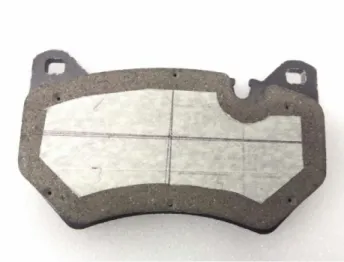
The design of the brake pad is done through Solidwork 2016 software. In this way it is easy to asses points 2,3. The design as depicted in Figure (11)

29 Figure 11: 1:1 Scale brake pad

The pad is represented in a 1:1 scale and the attribution of the material for the FEM analysis is given at the end as last step.

2.Evaluation of areas

Once the 3D-model is created, its surface has been calculated in mm2and then has been divided in parts according to predefined models: equal areas, offset perimeter, vertical and horizontal stripes, quarters, 1/6 of quarters . Different kind of measures are taken and with different approaches in order to get different aspects results.

For each type of measure a double test is done and corresponding Tables are created. The first test is limited to the pad itself, meanwhile the second on the system totality.

3.Surface division and conductive test

The main purpose of this procedure is to get as many concrete values as possible for a better material estimation. The measures are always done with the LRC instrument and set at the frequency of 12Hz. In the first approach it is important t understand if the pad is made up of a conductive or insulator material, so for this test the R/Q modes was adopted. The two probes are connected respectively one to fixed point such as the eyelet present on the pad plate and the other on the point of interest by applying a finger pressure. Here in Table(5) are shown the values corresponding the each selected quarter of area the 1/24 area analysis of the resistances expressed in ohm.

30 R [Ω] 1st quarter values 2nd quarter values

5.01 3.81 8.56 3.65 hole 5.26

2.42 3.54 3.76 4.35 6.75 4.34

3rd quarter values 4th quarter values

5.01 6.23 9.01 6.01 4.76 3.74

5.68 6.47 3.62 2.58 6.46 3.5

Table 5: Resistance values of the pad divided in 24 parts

It is noticeable that one slot is characterized by a “hole”, this due to the pad shape. In this particular case in that spot was not possible to get a value. Since a small resistance has been found we assume the pad to be composed of the mixture of materials that consider as a whole is conductive.

In Figure (12) is shown how the four quadrant are divided in and some spots where measurement have been taken. Finger pressure is not present for a better understand of the images. Important to notice is that the eyelet is always the same and not interchanged with the other one.

31 4.Impedance control

Conductivity is established, so the next step is to change mode and pass from R/Q to R/C one. This switch permits to obtain resistance and capacitance of the respective pad. Now the system changes, it is no more only the brake pad, but the set up of brake disc and pad The impedance measurements are calculated later once all R/C values are collected.

The different configurations are: a) 1/4 division (4 values)

b) left- right division (2 values) c) up-down division (2 values)

d) 1cm offset from perimeter, both cases (2 values)

e) 1,5cm vertical cut-off on both sides and vice versa (2 values) f) 2,5 cm horizontal cut-off both sides and vice versa (2 values)

All the values collected in Tables are then compared highlighting the relation between the absolute values of the impedance (Z complex number) and the corresponding areas (A). For a better evaluation of these values, the position of probes and pad on the disc are always the same. They have been marked in order to reduce position errors

For example test “a” is made by covering with an insulating Scotch tape each time 3 of the 4 sections of the surface leaving undercover the interested area. The measure is taken connecting the two probes respectively to the eyelet of the pad pate and a fixed point of the disc. This is done for each quarter.

5.First approach :Impedance analysis

a)in this test the quarter pad sectors are considered. Three quarters are covered with scotch tape meanwhile the remaining one leaved uncovered.

32 Since brake pressure should not act any kind of weight is not used. The only weight acting on the system is the pad one. Figure (13) highlights the setup of the impedance measurement.

Figure 13: First quarter impedance measurement

The four impedances results obtained are: and shown in Table (6)

where the quarters are defined as:  1 = top left quarter

 2 = top right quarter  3 = bottom left quarter  4 = bottom right quarter

and the Graph (1) comparison is: Impedance/ quarter area R [Ω] X [Ω] 1st Quarter 52.82 0.107 2nd Quarter _{62.22 0.142} 3rd Quarter 62.51 0.034 4th Quarter _{48.14 0.118} Table 6: Four quarter impedance

33 Graph 1: Four quadrant impedance

b) this test divides the pad in two parts: left side and right side. In both configuration the impedance test is measured and shown in Table(7):

impedance/ half

area R [Ω] X [Ω]

Left [sx] 28.25 0.110378 Right [dx] 24.63 0.070617 Table 7: Half quarter impedance vertical case

For sake of simplicity scotch tape is not perfectly shaped along the pad border as it had been done for the quarter configuration, but with some excesses (in Figure(14)possible is to be see the pre-cut stage where scotch tape is). The small excess doesn’t affect the measurement since the established insulation is guaranteed. 0 0.05 0.1 0.15 0 20 40 60 80 R e ctan ce [ Ω ] Resistance [Ω]

Z/ quarter impedance

34 c) is the same test as case b where the pad is divided in two equal parts: upper part and bottom part. For upper and bottom part is intended the portion of pad area divided by an horizontal line. The result are written in Table(8):

impedance/ half

area R [Ω] X [Ω]

Upper part 19.26 0.14744

Bottom partr 25.36 0.120633 Table 8: Half quarter impedance horizontal case

Since case b) and c) have similar results in terms of impedance, just one Graph (2) is performed:

Graph 2: Case b and c impedance comparison

d) in this case the border is analyzed. A 1cm border is defined as region to study. Two opposite configurations seen in Figure (15a, 15b) have been set and measured. The impedance values are represented in Table(9):

impedance/Border R [Ω] X [Ω] OutsideBorder 15.39 0.055722

Inside Border 20.85 0.382521 Table 9:Border impedance

0 0.1 0.2 15 20 25 30 R e ac tan ce [ Ω ] Resistance [Ω]

Z / half impedance

35

The cuts of the scotch are made directly with a sharp knife on the pad. Moreover during setup in order not to scrap, produce cavities or small holes on the surface a really sharp knife has beed adopted with a small pressure applied.

Figure 15b: Inside 1cm border impedance

The last two examples are related to the horizontal and vertical relative motion between rotor and stator, respectively disc and pads. Assuming the disc fixed, the pad is the relative moving element.

e) left-right contact depicted in Figure(16) allows to evaluate small contact due to non parallelism between pad and disc

36 Figure 16: Lateral extremes impedance

The opposite configuration is not pictured but can be easily imagined as the same as the previous one changing white part with black one and viceversa. From a numerical point of view Table (10) shows the measured values:

impedance/sides R [Ω] X [Ω] Vertical sided 77340 13.26964 Vertical inside 11.5 0.082497 Table 10: Left-Right/Center impedance

It is evident that when the inside part is taped and the sides considered, an open circuit is present since resistance is around 77 kOhm.

f) this configuration is characterized by an horizontal section (h sections). The main problem noticed is during up-down measure, the positioning of the pad: the changing of posing the pad let a contact of the sides or not a contact. Since we want to verify unwanted contacts, without knowing the real position, the pad has been positioned and then moved a bit rising the contact. In particular Figure(17) shows a central unwanted contact meanwhile the opposite configuration the other two possible unwanted contacts rising during not parallel set up. The values of this two configurations are inserted in Table(11)

37 Figure 17: Horizontal stripes

impedance/h-sections R [Ω] X [Ω]

Horizontal sides 589 0.11264 Horizontal inside 149.1 0.350122 Table 11: Horizontal section impedance

The last two configurations are the ones with a huge impedance gap between all the others and this is due to the fact that the contact is absent ( type e-sides) and the contact is less present even if same percentage of surface area are considered.

In the following Graph (3)e is depicted the Graph considering all impedance values expressing both R and Z in logarithmic scale:

Graph 3: Total configurations impedance measurement comparison 0.01 0.1 1 10 100 1 10 100 1000 10000 100000 Re act anc e [Ω ] Resistance [Ω]

z

z

38 The extreme right value is the one of no contact, meanwhile the rest represent a partial contact. This allows us to understand the difference between contact and no-contact, but not a clean difference between each type of contact.

A characterization curve of all the data has been elaborated through matlab software. An eighth order function is found ,shown in Figure(18), but it has an important non linear behavior. Due to this non-linearity it is not possible to establish a relationship between impedance over surface contact area.

Figure 18: 8th order impedance characterization curve

6.Second approach: impedance analysis through pressure

The first approach was not successful in terms of defining the resistivity of the pad so a new technique has been adopted. It differs from the previous one by two important factors:

 Pressure applied between disc and pad

 Point of connection of both probes

In this second test brake disc and brake pad are pressed together with the use of clamps in order to create a much wider contact between parts and so a better measurement. These new values are taken connecting the probes

39

respectively one to the same eyelet as the previous test, the other to the disc in eight different positions.

The eight spots are: left to the pad, right t the pad, hole cavity expressed by “0”, the other eyelet (left one), and the remaining four on the four elements inside the vented conducts. Here a Figure(19) for a better explanation:

Figure 19: Connection clamps points

To the top right the fixed probe and on the disc the clip points of the measurements indicated by numbers and letters.

The left eyelet setup has been measure in order to verify that in all the configurations the setup of the clamps wasn’t interfering.

Cases 1.1 and 1.2 differs by the number of clamps used to press the pad to the disc, in the first case four clamps (4PP), in the second two clamps (2PP). In both configurations, the central clamps are located on the pistons position, the other two at the pad extremity.

40

Figure(20) shows the two cases: 1.1 at left and 1.2 at right

Figure20: 4 pressure points versus 2 pressure points configuration

From the results reported in the following Tables (12) it is noticeable that in both cases the measure doesn’t depend on the contact position of the “free” probe both for resistances and capacitances.

New layouts are considered in cases 2, with four pressure points (4PP), where different contact areas are inspected: left side (HPVRC), right side (HPVLC), upper part (HPHUC) and lower part (HPHLC). These are the same configurations adopted in first approach.

In the last case, case 3, the pad is entirely covered with tape.

Case 1.1: 4 Pressure points (4PP)

Position/Z Left to the pad eyelet sx Right to the pad Positon 1 Position 2 Position 3 Position 4 Hole Pad R 0.7198 0.0028 0.7223 0.7213 0.7219 0.7218 0.7218 0.7269 [Ω] C -2.3529 over -2.4961 -2.6438 -2.2047 -2.2169 -2.1852 -2.4457 [μF]

Table 12a: 4 pressure points

Case 1.2: 2 Pressure points (2PP)

Position/Z Left to the pad eyelet sx Right to the pad Positon 1 Position 2 Position 3 Position 4 Hole Pad R 0.7936 0.0028 0.7868 0.7847 0.7838 0.7806 0.7815 0.7788 [Ω] C -1.8353 over -1.7973 -1.4673 -1.7871 -1.9002 -1.7998 -1.8674 [μF]

41

Case 2.1: Half pad far from the reference eyelet vertical covered with scotch tape (HPVLC) Position/Z Left to the pad eyelet sx Right to the pad Position 1 Position 2 Position 3 Position 4 Hole Pad R 1.27 0.0028 1.265 1.268 1.275 1.262 1.248 1.248 [Ω] C -0.2682 over -0.2796 -0.2300 -0.2681 -0.2511 -0.2481 -0.2823 [μF] Table 12c: 4 pressure points with partial insulation

Case 2.2: Half pad near to the eyelet vertical covered with scotch tape (HPVRC) Position/Z Left to the pad eyelet sx Right to the pad Position 1 Position 2 Position 3 Position 4 Hole Pad R 1.672 0.0028 1.633 1.635 1.623 1.626 1.626 1.608 [Ω] C -0.19835 over 0.13666 0.14094 0.17795 -0.1956 -0.1916 0.11543 [μF] Table 12d: 4 pressure points with partial insulation

Case 2.3: Half pad horizontally upper part covered (HPHUC)

Position/Z Left to the pad eyelet sx Right to the pad Position 1 Position 2 Position 3 Position 4 Hole Pad R 2.366 0.0027 2.292 2.262 2.208 2.216 2.199 2.195 [Ω] C 0.11173 over 0.0187 0.1296 0.10848 0.12991 0.11048 0.10745 [μF] Table 12e: 4 pressure points with partial insulation

Case 2.4: Half pad horizontally lower part covered (HPHLC)

Position/Z Left to the pad eyelet sx Right to the pad Position 1 Position 2 Position 3 Position 4 Hole Pad R 1.643 0.0028 1.619 1.521 1.497 1.473 1.408 1.423 [Ω] C 0.17736 over -0.19596 0.14363 0.10706 0.17626 0.12642 0.1561 [μF] Table 12f: 4 pressure points with partial insulation

Case 3:Complete insulated pad (TC)

Position/Z Left to the pad eyelet sx Right to the pad Position 1 Position 2 Position 3 Position 4 Hole Pad R 1.643 0.0028 1.619 1.521 1.497 1.473 1.408 1.423 [Ω] C 0.17736 over -0.19596 0.14363 0.10706 0.17626 0.12642 0.1561 [μF] Table 12g: 4 pressure points with total insulation

42

In the previous approach now impedances are evaluated, but since capacitance are small (μF) we can just consider resistances.

Starting from the four quadrant areas expressed in mm2 Table(13):

1st Quadrant [mm2] 2nd Quadrant [mm2]

1879.82 1870.93

3rd Quadrant [mm2] 4th Quadrant [mm2]

1870.14 1871.77

Table 13: Quadrant area values

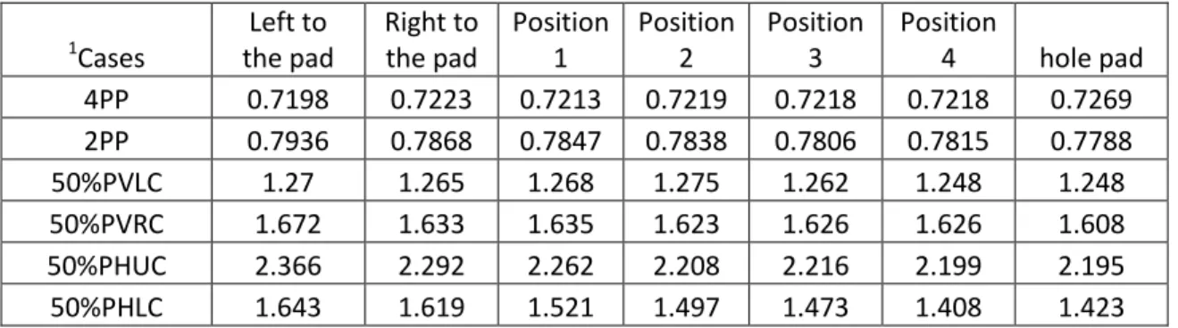
The total area (S) equals to 7492.66 mm2 and the synthetic resistance Table (14) not including case 3 is:

1 Cases Left to the pad Right to the pad Position 1 Position 2 Position 3 Position 4 hole pad 4PP 0.7198 0.7223 0.7213 0.7219 0.7218 0.7218 0.7269 2PP 0.7936 0.7868 0.7847 0.7838 0.7806 0.7815 0.7788 50%PVLC 1.27 1.265 1.268 1.275 1.262 1.248 1.248 50%PVRC 1.672 1.633 1.635 1.623 1.626 1.626 1.608 50%PHUC 2.366 2.292 2.262 2.208 2.216 2.199 2.195 50%PHLC 1.643 1.619 1.521 1.497 1.473 1.408 1.423

Table 14: Resistance values expressed in ohm of the over mentioned configurations

is possible to calculate the product resistance times contact surface area [Ω*mm2] : and represent it in Table (15).

Resistance times area [Ω*mm2] Cases Left to the pad Right to the pad Position 1 Position 2 Position 3 Position 4 hole pad 4PP 5393.217 5411.948 5404.456 5408.951 5408.202 5408.202 5446.415 2PP 5946.175 5895.225 5879.490 5872.747 5848.770 5855.514 5835.284 50%PVLC 4762.449 4743.699 4754.949 4781.199 4732.450 4679.950 4679.950 50%PVRC 6257.794 6111.829 6119.315 6074.402 6085.630 6085.630 6018.262 50%PHUC 8853.359 8576.458 8464.200 8262.137 8292.073 8228.460 8213.492 50%PHLC 6162.482 6072.464 5704.891 5614.873 5524.855 5281.056 5337.317

Table 15: Resistance times relative area values “PP”: pressure points;

“PVRC”: pad vertically right covered “PVLC”: pad vertically left covered

43

“PHUC”:pad horizontally upper covered “PHLC”:pad horizontally lower covered

Giving shape to the Table values in a Graph(4)

Graph 4: Resistance times area behavior

A linear behavior is highlighted in every configuration except from the 2.4 (“+” symbols) with a little decay of the values.

In each setup is considered:

Cases/parameters Min [Ω] Max [Ω] Delta [Ω] Mean [Ω] 4PP 5393.217 5446.415 53.19785 5411.627 2PP 5835.284 5946.175 110.891 5876.172 50%PVRC 4679.95 4781.199 101.249 4733.521 50%PVLC 6018.262 6257.794 239.5324 6107.552 50%PHUC 8213.492 8853.359 639.8671 8412.883 50%PHLC 5281.056 6162.482 881.4263 5671.134 Table 16: Parameters comparison

4000 5000 6000 7000 8000 9000 10000 0 1 2 3 4 5 6 7 8 R e si stan ce [ Ω ] Number Case [#] 1.1 4 pressure points 1.2 2 pressure points 2.1 left side covered 2.2 right side covered 2.3 upper side covered 2.4 lower side covered

44

Considering three different mean values:

1. All cases except 2.3 = 5560.001 [Ω] 2. Cases 1.1 and 1.2 = 5643.900 [Ω] 3. All cases = 6035.481 [Ω]

Mean number 2 is taken as reference, and in terms of percentage, the other two differs respectively: 1 by 1.5% and 3 by 8%. The second percentage is higher due to case 2.3 where the contact is in worst condition since clamps are all located externally to the disc.

Now resistivity can be calculated with (2.4) as:

where the height of the pad is =10mm, and at the numerator is taken mean value number 2

The parameter of our interest is conductivity

3.1 Capacity test with frequency sweep

When braking is not requested by the driver, any contact is established between the rotor and stator and an air gap is present. The air gap can be seen as an insulator and a capacitor is made up: the two armature are respectively rotor and stator, meanwhile the dielectric in the middle is air.(cool or hot) Since the rotor disc tested has not a flat surface but characterized by slots and drills, it is important to measure how capacitance behaves in different sections of the disc.

45

To realize this test, the brake pad is covered with a layer of scotch tape and settled on the disc surface. The LCR instrument probes are connected to the fixed position of the disc and to the eyelet of the pad. Frequency is very important in order to evaluate capacity, so measurement have been taken at three frequencies: 12Hz, the lower one the instrument can handle, 50 Hz, the common European frequency and 1kHz.

Three drills are present on the disc and for a better probes contacts the examined one is the one left to the fixed disc probe position. In particular five different position, as shown in Figure (21 a, b, c, d, e) are set:

1. Pad right to the designated slot 2. Pad above half right slot 3. Pad above the slot 4. Pad above half left slot 5. Pad left to the designated slot

In the photos below are represented the 5 configuration listed before:

Since the capacitance value is really small is important to be sure that the capacitance measurements are not affected by errors. To avoid this possible issue the used procedure is:

First place the pad over the disc in the correspondent position. Then fix the clamps respectively one on the disc previously defined reference point and the other one to the reference pad eyelet (right eyelet).

46

Once the system is fixed is possible to apply the frequency sweep. Three values of capacitance are taken. The process is finished, and the new position configuration can be performed.

Before any numerical analysis, the five cases can be divided in three groups: group 1 where there is not interaction between slot and pad (position 1 and 5), group 2 where there is partial Interaction (position 2 and 4) and group 3 where maximum interference should occur (position 3).

Figure 21b: Pad above half right slot

Figure 21c: Pad above the slot

47

From Table (17) is evident that even changing the frequency, the obtained values are of the same order of magnitude (nF) This means that the established set up doesn’t interact with the disc surface shape .

Frequency/position 12Hz 50Hz 1kHz Position description P1=PRS 0.56 nF 0.65 nF 0.49 nF Pad right to slot

P2=PAHRS 0.53 nF 0.62 nF 0.46 nF Pad above half right slot P3=PAS 0.56 nF 0.62 nF 0.49 nF Pad above slot

P4=PAHLS 0.59 nF 0.41 nF 0.49 nF Pad above half left slot P5=PLS 0.58 nF 0.42 nF 0.49 nF Pad left to slot

Table 17: Capacitance frequency sweep results

Once established that the rotor surface design doesn’t interact with the interested measures, new tests have been made considering the total disc-pad system.

Disc-pads electric circuit test

The aim of this test is to evaluate through capacitance measures the possibility to detect two threshold values for the three possible working conditions:

 No contact between pads and disc

 Contacts between both pads and disc