Searching for outflows signatures in sdss spectra of x-ray selected, obscured agn in the cosmos field

(1)

ALMA Mater Studiorum

Universita` degli Studi di Bologna

SCUOLA DI SCIENZE

!

Corso di Laurea Magistrale in Astrofisica e Cosmologia

!

Dipartimento di Fisica e Astronomia

!

Searching for outflows signatures in SDSS spectra of X-ray

selected, obscured AGN in the COSMOS field

!

Elaborato Finale

!

Candidato: Relatore:

Chiar.mo Prof.:

Giustina Vietri Andrea Cimatti

!

Co-relatore:

Dott.ssa Marcella Brusa

!

Sessione II

(2)

SOMMARIO

Contesto scientifico e scopi É ormai ritenuto molto probabile che al centro della maggior parte delle galassie si trovi un buco nero supermassiccio. La stretta corre-lazione tra la massa del buco nero e la dispersione delle velocità nel bulge galattico, nota come relazione M-σ, suggerisce che la formazione della galassia e del buco nero al suo centro siano tra loro collegate. La presenza di un buco nero (BN) supermassic-cio infatti ha un’importante conseguenza sulla storia evolutiva della galassia stessa, in quanto attraverso una fase di accrescimento può dar vita ad un Nucleo Galattico Attivo (AGN), che rilascia una grande quantità d’energia sotto forma di radiazio-ne e può produrre venti, spinti dalla pressioradiazio-ne della radiazioradiazio-ne, che influenzano la vita della galassia e del BN stesso. Questi venti interagiscono con l’ambiente della galassia ospite, portando alla formazione di flussi di gas su larga scala, che possono influenzare la massa finale della galassia. Infatti questi flussi di materia, che possono essere sotto forma molecolare, neutra e ionizzata, possono essere condotti al di fuori del bulge, bloccando la crescita del BN e la formazione di stelle nella galassia. Senza il gas necessario alla formazione di nuove stelle, la galassia ospite diventa un insie-me di stelle vecchie che fanno apparire la galassia più arrossata, giungendo cos`ı alla cosiddetta fase red and dead. Esaminando la riga d’emissione proibita dell’ossigeno, [OIII]λ5007, che viene prodotta in un ambiente a bassa densità, chiamato Narrow Line Region (NLR), è possibile tracciare la cinematica del gas ionizzato in questa regione dell’AGN. La FWHM di questa riga è in genere pari a ∼400-500 km s-1_,

quindi un eventuale allargamento o asimmetria del profilo di riga `e il risultato di un forte gradiente di velocit`a o di cinematica disturbata.

Nel nostro lavoro di tesi abbiamo deciso di esaminare AGN selezionati in X, con lo scopo di identificare i flussi di gas ionizzato attraverso la riga proibita dell’ossigeno, [OIII]λ5007.

Metodi e campione utilizzato Partendo dal campione di AGN presente nella survey di XMM-COSMOS, abbiamo cercato la sua controparte ottica nel database DR10 della Sloan Digital Sky Survey (SDSS), ed il match ha portato ad una selezione di 200 oggetti, tra cui stelle, galassie e quasar. A partire da questo campione, abbiamo selezionato tutti gli oggetti con un redshift z<0.86 per limitare l’analisi agli AGN di tipo 2, quindi siamo giunti alla selezione finale di un campione di 30 sorgenti. L’analisi spettrale `e stata fatta tramite il task SPECFIT, presente in IRAF. Abbia-mo creato due tipi di Abbia-modelli: nel priAbbia-mo abbiaAbbia-mo considerato un’unica componente per ogni riga di emissione, nel secondo invece `e stata introdotta un’ulteriore com-ponente limitando la FWHM della prima ad un valore inferiore a 500 km s-1_{. Le}

righe di emissione di cui abbiamo creato un modello sono le seguenti: Hβ, [NII]λλ 6548,6581, Hα, [SII]λλ 6716,6731 e [OIII]λλ 4959,5007. Nei modelli costruiti ab-biamo tenuto conto della fisica atomica per quel che riguarda i rapporti dei flussi teorici dei doppietti dell’azoto e dell’ossigeno, fissandoli a 1:3 per entrambi; nel caso

(3)

del modello ad una componente abbiamo fissato le FWHM delle righe di emissione; mentre nel caso a due componenti abbiamo fissato le FWHM delle componenti stret-te e larghe, separatamenstret-te. Tenendo conto del chi-quadro otstret-tenuto da ogni fit e dei residui, è stato possibile scegliere tra i due modelli per ogni sorgente. Considerato che la nostra attenzione è focalizzata sulla cinematica dell’ossigeno, abbiamo preso in considerazione solo le sorgenti i cui spettri mostravano la riga suddetta, cioè 25 oggetti. Su questa riga è stata fatta un’analisi non parametrica in modo da utilizza-re il metodo proposto da Harrison et al. (2014) per caratterizzautilizza-re il profilo di riga. Sono state determinate quantità utili come il 2◦ _{e il 98}◦ _{percentili, corrispondenti}

alle velocit`a massime proiettate del flusso di materia, e l’ampiezza di riga contenente l’80% dell’emissione.

Risultati L’analisi spettrale restituisce il flusso, le FWHM e i centroidi di ogni ri-ga d’emissione inserita nel modello. Abbiamo utilizzato i flussi dell’ [OIII]λ5007, [NII]λ6731, Hα e di Hβ per costruire il diagramma diagnostico di Baldwin, Phillips e Terlevich (BPT), utile per classificare gli oggetti in base alla ionizzazione delle righe. E’ stato possibile costruirlo per 12 sorgenti. Per cercare correlazioni tra i flussi di gas uscenti e l’AGN, abbiamo confrontato le FWHM delle componenti larghe dell’[OIII] con la luminosità totale della riga dell’ossigeno e con la luminosità bolometrica del-l’AGN. Abbiamo confrontato i nostri risultati con quelli in letteratura, ottenendo un intervallo di valori per la FWHM consistente con quelli dei campioni utilizzati nel confronto. Per indagare sull’eventuale ruolo che ha l’AGN nel guidare questi flussi di materia verso l’esterno, abbiamo calcolato la massa del gas ionizzato presente nel flusso e il tasso di energia cinetica, tenendo conto solo delle componenti larghe della riga di [OIII] λ5007. Per la caratterizzazione energetica abbiamo considerato l’ap-proccio di Cano-Diaz et al (2012) e di Heckman (1990) in modo da poter ottenere un limite inferiore e superiore della potenza cinetica, adottando una media geome-trica tra questi due come valore indicativo dell’energetica coinvolta. Confrontando la potenza del flusso di gas con la luminosità bolometrica dell’AGN, si è trovato che l’energia cinetica del flusso di gas è circa lo 0.3-30% della luminosità dell’AGN, consi-stente con i modelli che considerano l’AGN come principale responsabile nel guidare questi flussi di gas.

Applicazioni future La nostra analisi si basa su spettri non spazialmente risolti, questo non ci permette di avere delle informazioni spaziali riguardo all’estensione dei flussi di gas. Quindi l’uso di spettroscopia risolta è necessaria per effettuare un’analisi decisamente migliore e più utile, ai fini di caratterizzare in modo più veritiero la cinematica del gas preso in esame. In più è possibile considerare un numero maggiore di oggetti in modo da dare una valenza statistica ai risultati ottenuti o utilizzare una banda di osservazione diversa come l’infrarosso (IR), per lo studio di AGN a più alto redshift, in quanto in questo caso la riga dell’[OIII] risulta essere spostata nella banda del vicino infrarosso (NIR).

(4)

List of Figures

1.1 Scheme of an AGN continuum spectrum in diﬀerent types of AGN. 7 1.2 (Top panel) It is illustrated a model of AGN. (Medium panel)

The AGN emission from diﬀerent locations and a schematic description of the Unified Model (Bottom panel) (credit: Brooks/Cole Thomson Learning) . . . 10 1.3 BPT diagram from Chen et al 2009. The dotted curve defined by

Kauﬀmann et al. (2003a) and the dashed curve defined by Kew-ley et al. (2001) show the separation among starforming galaxies, composite galaxies, and AGNs. The solid line defined by Shuder et al. (1981) shows the separation between LINERs and Seyfert 2s. . 13 1.4 The distribution of galaxies (SDSS sample) in the present-day

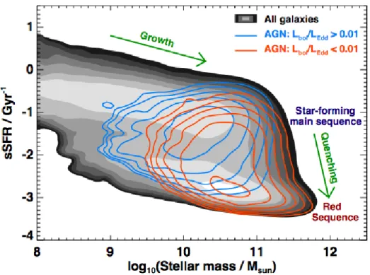
uni-verse. In grey there are represented all the galaxies, with the ex-istence of two regions: main sequence of star forming galaxies and a red sequence of red and dead galaxies. The blue and red con-tours represent the distributions of high and low Eddington-fraction AGN) (Heckman et al. 2014). . . 14 1.5 A scheme of the galaxy formation mechanism (Hopkins et al.

2008a) . . . 17 1.6 Galaxy luminosity function in the K (left) and bJ (right)

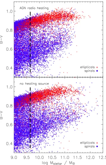
photo-metric bands. The solid line represents the galaxy luminosity func-tion with radio mode feedback; the long dashed line represents the galaxy luminosity function without feedback. . . 19 1.7 The B-V colours of model galaxies vs stellar masses with (top) and

without (bottom) radio mode feedback. Red triangles and blues cir-cles corrispond to early and late morphological type respectively. The thick dashed lines mark the resolution limit to which morphol-ogy can be determined in the Millennium Run and it corrispond to the stellar mass of 4 x 109 _M

⊙ . . . 20

(7)

iv LIST OF FIGURES

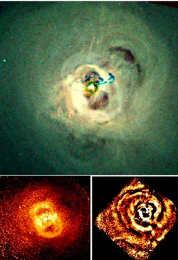
1.8 (Top panel) Chandra X-ray image of the Perseus cluster. Red-green-blue indicates soft to hard X-rays. The dark blue filaments in the center are likely due to a galaxy that is falling into NGC 1275, the giant galaxy that lies at the center of the cluster. (Lower Left) Pressure map derived from Chandra imaging X-ray spectroscopy of the Perseus cluster. Note the thick high pressure regions containing almost 4PV of energy surrounding each inner bubble, where V is the volume of the radio-plasma filled interior (Fabian et al 2006). (Lower Right): unsharp-masked image showing the pressure ripples or sound waves.. . . 22

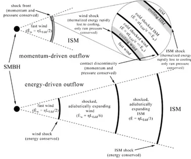
1.9 Schematic representation of momentum-driven (top) and energy-driven (bottom) outflows. In both cases a fast wind impacts the interstellar gas of the host galaxy, producing an inner reverse shock slowing the wind, and an outer forward shock accelerating the swept-up gas. In the momentum-driven case, the shocks cool to become isothermal. Only the ram pressure is communicated to the outflow, leading to very low kinetic energy. In an energy-driven outflow, the shocked regions do not cool. They expand adiabati-cally, communicating most of the kinetic energy of the wind to the outflow (Zubovas & King 2012) . . . 24

1.10 Recent calibration of M-σ relation from Gültekin et al 2009. Differ-ent galaxy types are indicated with differDiffer-ent colors and the symbols indicate the method of BH mass measurement: stellar dynamical with pentagrams, pas dynamical with circles and masers with as-terisks . . . 27

1.11 Galaxy-integrated spectra from Harrison et al. 2012. The spectra are shifted to the rest-frame, around the [OIII]λλ4959,5007 emis-sion line doublet. (Top panel) RG J0302+0010 exhibits a redshifted component with respect to the narrow component. (Bottom panel) SMM J1237+6203 exhibits a blueshifted component with respect to the narrow component. In both panels the red lines represent the best-fit, blue dashed lines represent the narrow component and green dashed lines represent the broad component.. . . 30

1.12 Scheme of a possible interpretation of the observations of the broad [OIII] emission lines. (For more details see the current subsection) 31

(8)

LIST OF FIGURES v

2.1 (upper left panel)The image combines data collected by the EPIC instrument on board XMM-Newton at energies [0.5-2] keV (red), [2-4.5] keV (green) and [4.5-10] keV (blue) (Cappelluti et al. 2009). (upper right panel) The image shows the 0.9 square degree COS-MOS field captured though in X-ray by Chandra (Elvis et al. 2009) at energies [0.5-2] keV (red), [2-4.5] keV (green) and [4.5-7] keV (blue) (bottom left panel) The image shows a composite, three-colour view of the COSMOS field, observed with Spitzer/MIPS at 24µm (blue) and with Herschel/PACS at 100 µm (green) and 160 µm (red) (credit: ESA / NASA / JPL-Caltech / PEP Key Programme consortium / Dieter Lutz). (bottom right panel) The VLA-COSMOS field is represented (Schinnerer et al. 2007) . . . . 39

2.2 Column 1: COSMOS IAU designation; Column 2: XMM-COSMOS identifier number (from Cappelluti et al. 2009); Columns 3-4: coordinates of the optical/IR counterpart; Columns 5-7: X-ray fluxes in the soft, hard, and ultra-hard bands (from Cappelluti et al 2009); Column 8: flag identifying the sources included in the flux-limited sample (1) or not (0); Column 9: X-ray hardness ratio, HR; Column 10: Chandra-COSMOS identifier number (from Elvis et al.2009); Column 11: flag for the optical identification, accord-ing to the classes described in the text: sources flagged with 1 are the reliable counterparts; sources flagged with 2 are the ambiguous counterparts; sources flagged with 0 are statistically not identified. Column 12: identifier number from Capak et al. 2007 catalog; Column 13: identifier number from the Ilbert et al. 2009 catalog; Columns 14-15: the r-band and I-band magnitudes (AB system, from Capak et al. 2007); Column 16: K-band magnitude (AB sys-tem, from McCracken et al. 2010); Column 17-20: magnitudes in the four IRAC channels (AB; from Ilbert et al. 2009); Column 21: MIPS 24 µm magnitude (AB, from Le Floch et al. 2009); Column 22: spectroscopic redshift; Column 23: spectroscopic classification: 1= BL AGN; 2= NL AGN; 3= normal/star-forming galaxy; Col-umn 24: origin of the spectroscopic redshifts. The code for the source of the spectroscopic redshift is the following: 1: SDSS; 2: MMT (Prescott et al. 2006); 3, 4: IMACS runs (Trump et al.2007, 2009); 5: zCOSMOS 20k catalog (Lilly et al. 2007); 6: zCOSMOS faint 4.5k catalog; 7; Keck runs; Column 25: photometric redshift (from Salvato et al. 2009). . . 42

(9)

vi LIST OF FIGURES

2.3 (left panel)Redshift distribution of the extragalactic XMM-COSMOS counterparts in ∆z=0.05. Open histogram contains all sources with spectroscopic or photometric redshift available; filled histogram contains all sources with spectroscopic redshift. (right panel) Spectroscopic breakdown of the sample (open histogram) in the three classes discussed in the text: BL AGN (blue filled his-togram), NL AGN (red upper histogram) and normal/SF galaxies (green filled histogram). In the bottom right panel it is repre-sented the distribution of the sources with photometric redshift only (cyan). The yellow filled histogram represent the redshift dis-tribution for the high-z obscured AGN candidates.(From B10) . . . 43

2.4 Luminosity-redshift plane for the sources with spectroscopic red-shift detected in the soft band (left panel) and hard band (right panel). In both panels blue circles are AGN 1, red circles are AGN 2 and green circles are normal/SF galaxies.From B10 . . . 44

2.5 DR10 SDSS/BOSS sky coverage (taken from www.sdss3.org/dr10/) 45

2.6 Three examples of spectra at low, medium and high redshifts: a starburst galaxy with z_{∼0.24 (}top panel), a QSO broadline with z∼0.81 (medium panel) and QSO broadline with z∼2.7 (bottom panel) . . . 49

2.7 The two-square-degree COSMOS field as seen by XMM-Newton (filled black circles) and SDSS (filled green circles). The sample of 194 sources, resulting from the cross-correlation be-tween XMM-COSMOS and SDSS, is represented as filled red circles. North is up, East is right. . . 50

2.8 Redshift distribution of the XMM-COSMOS sample cross-correlated with SDSS DR10 database, in ∆z=0.05. Based on com-bined optical and X-ray classification there are three classes: Nor-mal/SF galaxies (filled blue), Narrow Line AGN (filled red) and Broad Line AGN (filled green) . . . 52

2.9 Luminosity-redshift plane for all sources of the new sample, in the hard band. Blue circles are Normal/SF galaxies, red circles are NL AGN and green circles are BL AGN . . . 52

(10)

LIST OF FIGURES vii

2.10 (Left panel) Examples of SED decompositions for unobscured AGN (upper panels) and obscured ones (bottom panels). Black circles are rest-frame fluxes corresponding to the observed bands used to constrain the SED. Purple and blue lines correspond to the galaxy and the AGN template found as best-fit solution through the χ2

minimization, while the black line shows their sum. Pink and cyan shaded areas show the range of the SED template library within 1σ of the best-fit template, and light gray their sum. . . 54

2.11 SFR versus stellar mass. The green circles represent BL AGN, the red NL AGN and blue normal/SF galaxies . . . 55

2.12 Bolometric correction as a function of the bolometric luminosity in the [2-10]keV band for type-2 AGN sample. Blue diamonds refer to values determinated by means of the best-fit relation described in Lusso et al. 2012. Magenta diamonds refer to those described in Marconi et al 2004 . . . 57

3.1 Example of database file containing the initial guesses for parameters. 63

3.2 (Upper panel) Zoom in the regions of [OIII] of the source XID5626. The black solid curve represent the original spectrum and the red solid one is the best-fit to the data obtained from one component model fitting. (Bottom panel) Zoom in the regions of [OIII] of the source XID54517. The black solid curve and the red solid one have the same meaning as above. Under each spectrum the residuals with respect to the best fit are shown. . . 66

3.3 In all panels is represented a zoom in the region of [OIII]. In the left panels are represented the best-fit to the data (violet solid curve) of one component model of XID5112 (upper left panel), XID5435 (bottom left panel). In the right panels the best-fit to the data (blue solid curve) of the two components model of the same sources are shown. The red dot-dashed curve represents the narrow compo-nent with FWHM<500 km/s in each panel; the green dashed curve represents the broad component in each panel. Under each fit the residuals with respect to the best fit are shown. . . 69

(11)

viii LIST OF FIGURES

3.4 In all panels is represented a zoom in the region of Hα. In the left panels are represented the best-fit to the data (blue solid line) using the one component model of XID5112 (upper left panel), XID5435 (bottom left panel), The red dot-dashed curve represents the narrow component . In the right panels best-fit to the data (blue solid line) using two components model of same sources are shown. The red dot-dashed curve represents the narrow component with FWHM<500 km/s in each panel; the green dashed curve represents the broad component in each panel. Under each fit the residuals with respect to the best fit are shown. . . 70

3.5 Illustration of non parametric velocity definitions in [OIII]λ5007 emission line profile of XID5318. The vertical dot-dashed lines show diﬀerent percentiles to the flux contained in the emission line profile (from the left to the right: 2th, 5th, 10th, 50th, 90th, 95th and 98th). The horizontal line represents W80, the line width that

contains 80% of the flux. . . 74

3.6 Average [OIII] profile of sources with one single component result-ing in individual fittresult-ing. This profile shows a blue asymmetric wresult-ing well modelled by a broad component (red dot-dashed curve). The narrow component is represented with green dot dashed curve. The fit produced by combining these two components is shown with blue solid curve. . . 76

3.7 Average [OIII] profile of sources with a broad component resulting in individual fitting. This profile shows a blue asymmetric wing well modelled by a broad component (red dot-dashed curve). The narrow component is represented with green dot dashed curve. The fit produced by combining these two components is shown with blue solid curve. . . 77

3.8 Average [OIII] profile of all sources with [OIII] emission line de-tected. This profile shows a blue asymmetric wing well modelled by a broad component (red dot-dashed curve). The narrow compo-nent is represented with green dot dashed curve. The fit produced by combining these two components is shown with blue solid curve. 78

(12)

LIST OF FIGURES ix

4.1 BPT diagram. [OIII]λ5007/ Hβ vs [NII]λ6584/Hα of 12 sources of our sample. Red solid line represents the criteria used to discrim-inate between NLAGN and HII galaxies from Kewley et al 2001. Green dashed line indicates that used by Kauﬀman et al 2003. Blue triangles represent the sources fitted with one component model; red diamonds represent sources fitted with two components model, with both narrow and broad components; green squares represent the narrow and broad components of sources fitted by two compo-nents model. Violet circles represent sources fitted with a narrow or a broad component for each line. . . 80

4.2 FWHM of the broadest component of [OIII]λ5007 line vs total [OIII]λ5007 luminosity. The blue circles marked the broadest com-ponents. Single components of [OIII]λ5007 with FWHM> 500 km s-1 _{of those sources well fitted by one component model are also}

plotted (magenta circles). We reported as yellow circles the re-sults of Brusa et al. 2014 of z_{∼ 1.5 obscured QSOs from XMM} COSMOS. The orange filled squares represent the average values of the broad FWHM of SDSS population studied by Mullaney et al 2013 in two luminosities ranges (1040 _{<L[OIII]< 10}41 _{erg s}−1

and 1041.5 _{<L[OIII]< 10}42.5 _{erg s}−1_{). Violet-red circle represent}

the stacked spectrum of ∼110 XMM-COSMOS Type2 QSOs (in the range z=0.5-0.9). 8 dust-reddened QSOs at z=0.5-1, from Ur-rutia et al 2012 are plotted as red filled squares. Green diamonds represent radio-quiet Type-2 QSOs at L[OIII]> 1043 _{erg s}−1 _from

Liu et al 2013( in this case we plotted the W80 non parametric

width, which can be used as FWHM of the lines). Violet diamonds represent 15 type 2 QSOs from the SDSS studied in Greene et al 2009,2011 with L[OIII]1042_{erg s}−1_. _{. . . .} ₈₆

4.3 FWHM of the broadest component of [OIII]λ5007 line vs the AGN bolometric luminosity. The blue circles marked the broadest com-ponents. The single component of [OIII]λ5007 with FWHM>500 km s-1 _{of those sources well modelled by the one component model}

are also plotted (magenta circles).As in the previous plot we re-ported the samples of Liu et al 2013 (green diamonds), Urrutia et al 2012 (red squares), Brusa et al 2014 (yellow circles). Black triangles represent the sample from Harrison et al 2012, which is composed of 8 SMG/ULIRGs at z_∼2. . . . 88

(13)

x LIST OF FIGURES

4.4 The mean value of kinetic power associated to outflows versus bolo-metric AGN luminosity. The blue circles represent the sources with [OIII]λ5007 broad component. Sources with only one significative component of [OIII]λ5007 emission-line profile with FWHM>500 Km/s (magenta circle) were plotted. The solid, the long-dashed, dotted and short- dashed lines represent the 100 %, 10 %, 5% and 1% ratios, respectively. . . 94 4.5 The mean value of kinetic power associated to outflows versus the

predicted kinetic output from SF. The blue circles represent the sources with [OIII]λ5007 broad component. Sources with only one significative component of [OIII]λ5007 emission-line profile with FWHM>500 km/s (magenta circle) were plotted. The solid, the long-dashed, dotted and short- dashed lines represent the 100 %, 10 %, 5% and 1% ratios, respectively. . . 96 5.1 Diagnostic diagrams showing the variation in ionisation state of

the gas in NGC 7130. The solid lines in the diagrams trace the the-oretical upper bound to pure star-formation (Kewley et al. 2001), the dashed line indicates the empirical upper bound to pure star-formation (Kauﬀmann et al. 2003). The smooth distribution of points from the pure star-forming region to the AGN region on the diagnostics is indicative of starburst-AGN mixing. . . 100 5.2 Map of the narrow component of Hα. (left) The white contours

identify the strongest gas outflow traced by the highly blueshifted [OIII] line (right) The white contours identify the highest velocity dispersion region, which is likely the region where the strong outflow interacts with the host galaxy disk. . . 101

(14)

List of Tables

2.1 Optical imaging information . . . 46 2.2 Optical spectroscopic information:SDSS vs BOSS . . . 47 2.3 Bolometric correction relations for X-ray selected Type-2

AGN sample in [2-10]keV band . . . 57 2.4 . . . 58 2.5 Final sample coordinates, redshifts, SFRs, stellar masses,

LogLx and LogLbol . . . 59

3.1 Vacuum wavelength of some atomic transitions . . . 64 3.2 Fit to the Hα, Hβ,[OIII]λ5007,[OIII]λ4959,[NII]λ6548,[NII]λ6581

with χ2 . . . 67 3.3 Fit to the Hα, Hβ,[OIII]λ5007,[OIII]λ4959,[NII]λ6548,[NII]λ6581

with χ2 and the velocity shift of broad component with respect to the narrow component. . . 72 3.4 Non parametric velocities: v2 or v98 and W80 . . . 75

3.5 FWHM and fluxes of [OIII]λ5007 in stacked spectra . . . 78 4.1 Decrement, E(B-V) and AV of narrow and broad components 83

4.2 Quantities useful to determine density of outflowing gas (Pradhan 1976). . . 90 4.3 Outflow kinetic power of the ionized gas derived from Eq.

4.14, Eq. 4.15 and the mean of the two values . . . 93 A.1 Objects classification . . . 105

(15)

Chapter 1

Introduction

One of the most active research areas in astrophysics is the study of the formation and evolution of galaxies. Even if some ideas are now widely ac-cepted, many questions on the formation and evolution of galaxies remain unanswered. The current paradigm of galaxy formation assumes that galax-ies grew out of primordial Gaussian density fluctuations, generated during inflation and amplified by gravitational instability acting on Cold Dark Mat-ter (CDM), the dominant mass component of the Universe. In this scenario structures form beginning with small objects which then merge to form ever larger structures: it is called bottom-up formation. Its competitor is top-down scenario, where hot dark matter is the main character. In this scenario large scale objects form first, which fragment into smaller objects. 1

Before the CDM cosmology became the favored cosmological model, many others appeared. Press and Schecther (1974) used a spherical model (Gunn & Gott 1972) to describe the evolution of a uniform, spherically sym-metric overdensity in an otherwise unperturbed universe and to predict the number of objects as a function of their mass M, basing on the idea that pri-mordial density perturbations were Gaussian fluctuations and evolved into bound objects with mass M, after they reached an amplitude greater than some critical value, δc. In this model the sequence of structure formation

is hierarchical: the universe fragments into low-mass clumps at high red-shift, following which a number of clumps merges into larger units at later times. But Press and Schecther involved a gas of self-gravitating mass in this scenario, there is as yet no dark matter.

White and Rees (1978), which may be considered the progenitors

1_{The observations favor the bottom-up scenario, thus only CDM will be discussed in}

the text.

(16)

2 CHAPTER 1. INTRODUCTION

of nearly all current theoretical models of galaxy formation, adopted a model based on the hierarchical clustering scenario proposed by Press and Schechter (1974) but with two new ingredients: dark matter and the cooling of baryons, in order to reproduce the structures we observe as galaxies. They proposed a two stage theory of galaxy formation with dark haloes forming in a dissipationless, gravitational collapse and galaxies forming inside these haloes, following the radiative cooling of baryons.

The first semy-analitical model of galaxy formation was produced by White & Frenk (1991), which included elements such as cold dark matter, gas cooling, star formation, feedback and stellar populations, at the root of today’s models.

The current standard model is based on a cold dark matter with a cos-mological constant Λ, that accounts for the presence of dark energy, a hypo-thetical force that appears to be accelerating the expansion of the Universe. According to the ΛCDM theory, the Universe was hot, smooth and homoge-neous immediately after the Big Bang. However small fluctuations in density began to appear and grow, which were characterized by the following density contrast:

δ = δρ ⟨ρ⟩ =

ρ_{− ⟨ρ⟩}

⟨ρ⟩ (1.1)

where ⟨ρ⟩ is the average density of the Universe and ρ is the perturbation density.

The medium was composed of cold dark matter, baryonic matter and radiation, which initially were coupled. The dark matter was the first com-ponent to decouple with radiation, since experiences only the weak and gravitational forces. After the decoupling, the dark matter began to col-lapse and the first potential wells were formed. The density fluctuations of baryon-radiation plasma oscillated until the baryonic matter decoupled from the radiation. Thereafter the matter fell into the potential wells cre-ated by DM, collapsed and condensed to form stars, i.e. Population III2_and

galaxies. Part of this gas was probably used to form a massive black hole (MBH). There are three possible scenario about its formation:

2_{. Population III (Pop III) stars are composed entirely of primordial gas, i.e. hydrogen,}

helium and very small amounts of lithium and beryllium. This means that the gas from which Pop III stars formed had not been ’recycled’ (incorporated into, and then expelled) from previous generations of stars, but was pristine material left over from the Big Bang. As such, these stars would have a [Z/H]_{∼ -10 and would constitute the very first generation} of stars formed within a galaxy. These Pop III stars would then produce the metals observed in Pop II stars and initiate the gradual increase in metallicity across subsequent generations of stars.

(17)

1.1. THE EMISSION OF AGN 3

• One star per galaxy more massive than 250 M⊙ forms then collapses

and gives rise to a MBH of 100 M_⊙

• If a globally unstable disk is formed then the unstable gas infalls to-wards the galaxy center and forms a supermassive star. The stellar core collapses and forms a BH of a few tens of M_⊙, which is embedded in what is left of the star thus it can grow by eating its surrounding and reach a mass of million solar masses.

• If a locally unstable disk is formed then the gas flows towards the galaxy center and stars start to form in this central region, giving rise to a dense stellar cluster. The collision between stars can produce a very massive star that collapses into a massive black hole.

These BH seeds, in place when the Universe was only few hundreds of Myr old, then will grow their mass through accretion of material and will begin the Supermassive Black Holes (SMBH) we observe today at the centre of the galaxies (with masses of 106− 109 _M_{⊙). When SMBHs grow through}

accretion of nearby matter, the gravitational potential of the accreted mass is converted into radiation making the central object luminous. In this case the SMBH is called active galactic nucleus (AGN) (Salpeter 1964, Lynden-Bell 1969, Shakura & Sunyaev 1973).

1.1 The emission of AGN

The AGN phase occurs when the BH is accreting matter. The gravi-tational field of the AGN draws the matter orbiting it inward, forming an accretion disk and leading to viscous heating and to an observational sig-nature in the emitted radiation. The rate at which energy is emitted by the nucleus, i.e. its luminosity, gives us the rate at which energy must be supplied to the nuclear source by accretion:

L = η ˙M c2 (1.2) where ˙M = dM/dt is the mass accretion rate and η is the mass-to-energy conversion eﬃciency, which determines the viability of accretion as a source of energy, and c is the speed of light.

The potential energy of a mass m at a distance r from the central source of mass M is

U = GM m

(18)

the rate at which the potential energy of infalling material can be converted to radiation is given by L_≈ dU dt = GM r dm dt = GM ˙M r (1.4)

Combining equations 1.2 e 1.4 follows that η ∝ M/r, which is a measure of the compactness of a system. Considering a characteristic scale of the BH, i.e. Schwarzschild radius RS = 2GM/c2, the energy available from a

particle of mass m falling to within this scale is:

U = GM m 5RS

= GM m

10GM/c2 = 0.1mc

2 _(1.5)

and this leads to a mass-to-energy conversion eﬃciency of 0.1.

The accretion onto a BH is limited by the eﬀects of the radiation pressure experienced by the infalling matter. As first pointed out by Arthur Edding-ton in the 1920s, this limit depends on the mass of the central source and the opacity of the infalling material. The so called Eddington luminosity is the observable quantity corresponding to the critical mass accretion rate and, supposing that the gas around the BH is fully ionized hydrogen and assuming spherical symmetry, is obtained by equating the outward radiation force

Frad =

LσT

4πr2_c (1.6)

to the inward force due to the gravity:

Fgrav =

GM mp

r2 (1.7)

where in equation 1.6 σT is the Thomson cross-section and in equation 1.7

M is the central object mass and mp is the proton mass. The Eddington

luminosity is therefore: LEdd = 4πGM mpc σT ≃ 1.3 10 38 M M⊙erg s −1 _(1.8)

Thus the Eddington accretion rate is: ˙

MEdd= LEdd/ηc2 (1.9)

Angular momentum considerations must take into account, since the or-biting material must lose angular momentum: the total angular momentum

(19)

1.2. OBSERVATIONAL PICTURE OF AGN 5

of the system must be conserved, thus the angular momentum lost due to matter falling onto the center has to be oﬀset by angular momentum gain of matter far from the center.

The physics underlying this angular momentum transport remains an active field of study, even if the problem seems to be now qualitatively understood. Balbus and Hawley (1992) involves a magnetic field with a component in the axial direction of the disk, which leads to a dynamically unstable situation so that angular momentum transport occurs. But an approximate solution to the problem was proposed by Shakura and Sunyaev (1973), applicable to geometrically thin optically thick accretion disks. The assumption is that the energy from accreted material is dissipated within a small region at its radius r and since the disk is optically thick, the spectrum is that of a black body with a temperature T(r). Gravitational potential energy is released at the rate GM ˙M /r and from the virial theorem, half of this goes into heating the gas and the other half is radiated away at the rate L:

L = GM ˙M

2r = 2πr

2_σT4 _(1.10)

where σT4 is the black body radiation formula for the energy per unit area and 2 πr2 _{is the disk area. This leads to a temperature at r:}

T ∝ (M ˙M )1/4r−3/4 (1.11) Taking into account how the energy is dissipated in the disk through viscosity and rewriting the relation in terms of Eddington accretion rate (eq. 1.9), the eq. 1.11 can be also written as follows:

T (r) = 6.3 105( ˙M / ˙MEdd)1/4 M8−1/4(

r RS

)−3/4 K (1.12) where RS is the Schwarzschild radius. From eq 1.12 one would expect

that the peak temperature of the accretion disk is lower for more massive BHs. The thermal emission from an AGN accretion disk is expected to be prominent in the UV spectrum with a temperature peak T_{∼ 10}5 _K.

1.2 Observational picture of AGN

A key observational aspect of AGN is the continuum spectral distri-bution, that ranges from radio to hard X-ray. The AGN spectral energy distribution (SED) shows the following features:

(20)

• Big blue bump (BBB): it covers the wavelength range from 4000˚A to 1000˚A. This bump is attributed to the thermal emission from the accretion disk surrounding the SMBH.

• The infrared bump: it is a broad feature with a peak at 10µm. This bump is thought to arise from reprocessing of BBB emission by dust with temperature in the range of 10-1800 K and at a range of distances from the central source (Phinney 1989).

• The near-infrared inflection: it appears as a dip between the two bumps.

• The submillimeter break: it marks a sharp drop in emission. The exact location of this feature and the size of the drop varies within the AGN population. In radio-loud objects the drop in power output is only ∼ 2 decades, while for the more common radio-quiet objects it may be_{∼ 5 or 6 decades (Elvis et et al. 1994). This part is associated} to synchrotron radiation from powerful jets in radio-loud AGN. • X-ray region: it can be divided in soft and hard X-ray band.

In the soft region there is the soft X-ray excess that may be the high energy continuation of the BBB. In the hard X-ray band the shape of the SED, a power law spectrum, is due to Compton upscattering of optical/UV photons by hot or nonthermal electrons of the corona above the disk. Superimposed on this power law are Fe Kα emission line at 6.4 keV and a Compton reflection hump above 10 keV. These two features are thought to be due to fluorescence and reflection from the accretion disk.

In figure 1.1 it is shown a schematic representation of the broad-band continuum spectral energy distribution seen in diﬀerent types of AGNs.

(21)

Figure 1.1: Scheme of an AGN continuum spectrum in diﬀerent types of AGN.

One of the first distinguishing observational properties of AGN is the presence of redshifted, time variable intensity emission lines with Doppler widths of order of 103 to a few of 104 km s-1.

These broad lines, such as hydrogen Balmer series lines Hαλ6563, Hβλ4861, Hγλ4340 and hydrogen Lyαλ1216, come from to the so called Broad Line Region (BLR). This region is assumed to be in photoionization equilibrium: the rate of photoionization is balanced by the rate of recombi-nation. Thus it is possible to infer physical parameters such as the diﬀerent number density of ions stage and the gas temperature. In general temper-atures of 104 _{K and densities of n}

e∼ 109 cm-3 are found. Since this value

of temperature corresponds to line widths of order of 10 km s-1, this means that line broadening is due to supersonic bulk motion of BLR, interpreted as an orbital motion about the central compact object. BLR provides therefore important insight into the BH.

There are also narrower forbidden and permitted lines but their widths and lack of variability suggest that they are originated from a region that is much larger and kinematically separated from BLR: the Narrow Line Region

(22)

(NLR). Photoionized by the UV/X-ray continuum radiation emitted by the central source, this region shows lines, such as [O III] λλ4959, 5007, [N II]λλ6548, 6583, [O I] λλ6300, 6364, [S II] λλ6716, 6731, that have FWHM of∼400-500 km s-1_{, and the presence of forbidden lines is indicative of gas}

densities of_∼103-105 cm-3, much lower than those of BLR.

1.2.1 AGN classification and Unified Model

The AGN phenomenon was first defined by means of optical spectra and two groups were identified: broad-line emission galaxies (or Type-1) and narrow-line emission galaxies (or Type-2).

The former are characterized by broad permitted lines such as Balmer lines, mainly Hα, Hβ, Hγ and Lyα, CIV, MgII, with line widths that indicate velocities of 103-104 km s-1 and by narrow forbidden lines such as oxigen [OII] and [OIII], and the nitrogen and neon [NII], [NeII] and [Ne IV], with typical velocities of a few hundred km s-1_{. The latter class is characterized}

by forbidden and permitted lines, which show the same narrow width. A further classification can be made according to the radio emission. AGN can be divided in radio loud, objects that produce large scale radio jets and lobes, and radio quiet, objects with radio ejecta energetically in-significant.

Recently various unification schemes have been developed to explain AGN as different appearances of the same underlying phenomenon. An-tonucci 1993 and Urry & Padovani 1995 proposed that there are basically radio quiet and radio loud AGN. For each type, different luminosities lead to different classes but all other differences are explained by different orien-tations to the observer.

In this scenario the basic idea is that the SMBH is surrounded by an optically thick torus, consisting of gas and dust. If the observer looks at the AGN through the torus then the broad-line region, nearby the central engine, is hidden by the toroidal material. As a consequence, the narrow-line region, far from the nucleus ( from 10 pc up to 100 pc from the center) is visible. At any other angles both the broad and narrow regions are visible. Analyzing radio quiet Seyfert, in the first case we have the Seyfert 2, in the second the Seyfert 1. According to unified model there is no real distinction between the two cases: Seyfert 2 are Seyfert 1 with hidden broad line region and occur in spiral galaxies.

A distinction between Seyfert 1 and Seyfert 2 can be also made in X-rays. It is based on the intrinsic absorption measurement in the soft X-ray band; the diﬀerences result from the amount of absorbing material close to the

(23)

central engine. The absorption is measured as a column density of hydrogen NHin the line of sight in atoms per cm2, taking into account the absorption

in our Galaxy.

The hydrogen column density of NH=1022 cm-2 was chosen as dividing

line from Seyfert 1, which, but not all, have lower absorption than this value, and Seyfert 2 which reside above of this value, but again not all (Panessa & Bassani 2002)

Another distinction can be made if we consider radio galaxies: broad line radio galaxies (BLRG) and narrow line radio galaxies (NLRG). These look like radio loud Seyfert but they seem to occur in ellipticals rather than spirals. In case of radio loud AGN, if the source is seen face-on, the spectrum is dominated by the jet and no lines are visible: we have the so called Blazar. In the following three panels there are represented an AGN portion of a galaxy (upper panel), the emitted particles from diﬀerent locations (medium panel) and what we see based on the orientation (bottom panel).

(24)

Figure 1.2: (Top panel) It is illustrated a model of AGN. (Medium panel) The AGN emission from diﬀerent locations and a schematic description of the Unified Model (Bottom panel) (credit: Brooks/Cole Thomson Learning)

(25)

1.2.2 Diagnostics based on emission lines

As it was described previously, there is no single signature of an AGN, but the most commonly distinguishing characteristics are found in optical band. Indeed still in the modern era of astronomy the most extensive studies of AGN activity in the local Universe have utilised optical spectroscopy (Heckman et al 2004, Ho 2008). Since the NLR extends beyond the obscured central region, optical spectroscopy is able to identify even heavily obscured AGN. The optical classification is not so eﬃcient in presence of significant host-galaxy dust and star formation, but in this case mid-IR spectroscopy, radio and X-ray observations can provide the identification of AGN.

Some galaxies show emission line spectra similar to those of Seyfert 2 galaxies, thus it is necessary to examine these emission lines in order to correctly classify an AGN spectroscopically. These Seyfert 2-like emission lines are often produced by massive gas clouds of ionized hydrogen, HII re-gions. Through the study of ionization level of various emission lines it is possible to discriminate between type 2 objects and HII/starburst galax-ies. Baldwin, Phillips & Terlevic (Baldwin et. al 1981) presented a clas-sification diagram, based on measured line ratios, to distinguish diﬀerent object classes: the BPT diagram. This tool compares the following flux ra-tio pairs: [OIII]5007/Hβ vs [NII] 6584/Hα. There are two commonly used BPT diagnostics: [SII]6717,6731/Hα vs [OIII]5007/Hβ and [OI]6300/Hα vs [OIII]5007/Hβ (Veilleux & Osterbrock 1987, Kewley et al 2006, Kauﬀmann et al 2003).

The [OIII]/Hβ line ratio is sensitive to the ionisation parameter and temperature of the line emitting gas, and is enhanced both in the presence of low metallicity stars, where a lack of metals prevents the nebula from cooling eﬃciently, and in the presence of an AGN due to the hard radiation field. But this degeneracy between pure star formation and AGN activity can be broken comparing this emission line ratio with another one. For example it is possibile to use the [NII]6584/Hα ratio which is sensitive to metallicity in star forming galaxies but the contribution from AGN radiation field causes this ratio to become enhanced.

As we previously mentioned, [SII]6717,6731/Hα and [OI]6300/Hα ratios can be used, since are also enhanced in the presence of hard ionising radiation field like the one of AGN in the BPT diagram with [NII]6584/Hα.

The same diagram can be used for type 1 AGN providing that only the narrow components of Balmer lines are considered (Stern & laor 2012a).

Below are listed the two demarcations found by Kauﬀmann et al. 2003a and Kewley et al. 2001 used to distinguish among starforming galaxies,

(26)

com-12 CHAPTER 1. INTRODUCTION

posite galaxies and AGNs in the BPT diagram with [OIII]/Hβ vs [NII]/Hα:

• (Kauﬀmann et al. 2003a)

log([OIII]/Hβ) = 0.61/(log([N II]/Hα)_{− 0.05) + 1.3} (1.13)

• (Kewley et al. 2001)

log([OIII]/Hβ) = 0.61/(log([N II]/Hα)_{− 0.47) + 1.19} (1.14)

In the figure 1.3 it is represented an example of a BPT diagram from Chen et al. 2009. The dotted curve is the demarcation found by Kauﬀmann et al. (2003a) and the dashed curve that found by Kewley et al. (2001). The solid line defined by Shuder et al. (1981) shows the separation between LINERs and Seyfert 2s.

Low-ionization nuclear emission galaxies (LINERs) show faint core lumi-nosities and strong emission lines originating from low ionized gas. LINERs are assumed to represent the link between HII regions and Seyfert galaxies: diﬀerent from Seyfert, LINERs can show [OIII] λ5007/Hβ <3 and in com-parison to HII regions, LINERs have stronger [NII] lines when compared to the Hα line flux.

LINERs have low luminosity and accretion rates, this leads to the idea that are not emitting through the same processes as the more active Seyfert and Quasar cores. The infalling matter will be optically thin at such low luminosity, thus they may be accreting with low radiative eﬃciency. Energy will be transported outward through flow of matter, thus these types of AGN are better described by models like Advection Dominated Accretion Flow (ADAF), where accreting gas is heated viscously and cooled radiatively but any excess heat is stored in the gas and transported in the flow (Ho 2008). ADAFs may be associated with jets.

(27)

Figure 1.3: BPT diagram from Chen et al 2009. The dotted curve defined by Kauﬀmann et al. (2003a) and the dashed curve defined by Kewley et al. (2001) show the separation among starforming galaxies, composite galaxies, and AGNs. The solid line defined by Shuder et al. (1981) shows the separation between LINERs and Seyfert 2s.

Optical spectroscopy is also eﬀective at identifying distant obscured AGN (Alexander et al 2008, Yan et al 2011), however the AGN emission-line diag-nostics move into near IR band at z>0.4, so it can be limited in identifying large numbers of AGN. The most eﬃcient identification of distant AGN is made with X-ray observations, since X-ray emission from star formation is typically weak. In presence of high absorbing column density, so high that not even X-ray photons can escape, IR and radio observations can help AGN identification (Hickox et al 2007, Bauer et al 2010).

(28)

1.3 AGN Galaxy co-evolution

In the present-day universe a bimodality sequence in the galaxy popula-tion is observed (Kauﬀmann et al 2003b):

• blue galaxies (Hubble late type), with on going star formation, low stellar surface density and characterized by a tigh relation between SFR and stellar masses: star forming main sequence (Brinchmann et al. 2004)

• red galaxies (Hubble early type), with little or absent star formation, large stellar masses and high stellar surface density

In figure 1.4 it is represented the relation between the stellar masses and the specific SFR of a sample of blue and red galaxies, at low redshift.

Figure 1.4: The distribution of galaxies (SDSS sample) in the present-day universe. In grey there are represented all the galaxies, with the existence of two regions: main sequence of star forming galaxies and a red sequence of red and dead galaxies. The blue and red contours represent the distributions of high and low Eddington-fraction AGN) (Heckman et al. 2014)

(29)

1.3. AGN GALAXY CO-EVOLUTION 15

Since this bimodality is a characteristic of the galaxy population out to at least z_{∼2 (Whitaker et al. 2013), it is possible to put this distribution} in a evolutionary context where the principal responsible for the move from blue to red seems to be the AGN, as many numerical simulations suggest. Moreover, we can put the diﬀerent AGN population in the same scenario and not just in a geometrical one.

1.3.1 The need for AGN feedback

The idea that there is a connection between the growth of the SMBH and its host galaxy has been put forward (Silk & Rees 1998, Granato et al. 2004, Di Matteo et al. 2005, Menci et al. 2008).

To understand what kind of role the AGN can have on the host galaxy, it is useful to compare the energy released by the growth of the BH and the binding energy of the galaxy. An important result turns out.

The binding energy can be expressed as follows:

Egal = Mgalσ2 (1.15)

where Mgalis the galaxy mass and σ is the velocity dispersion of the galaxy.

The energy released by the growth of the BH is:

EBH = ϵMBHc2 (1.16)

where ϵ is the radiative eﬃciency for the accretion process and it is ∼ 10%. Considering that the mass of the BH is observed to be MBH =

1.4 10-3_M

gal(Kormendy & Gebhardt 2001, Merritt & Ferrarese 2001, H¨aring

& Rix 2004) and that most galaxies have σ < 400 km s-1, the ratio EBH/Egal

is greater than 80. This means that the AGN can have an important eﬀect on the formation and evolution of the host galaxy.

As we already mentioned, the mass of a SMBH is only a small frac-tion of that of the host galaxy but we know that the two masses correlate. A tighter relation is found with the inner part of the galaxy, i.e. bulge, which suggests that galaxies hosting classical spheroids grew in concert with their BHs. A connection between the growth of the BH (via accretion) and the galaxy spheroid (via star formation) may be expected since both pro-cesses are driven by the availability of cold gas on nuclear scales, which is provided by the host galaxy or the larger-scale extragalactic environment. The majority of the mass accretion onto BHs occured at high redshift, at z>0.1(Marconi et al 2004, Hopkins et al. 2007, Merloni & Heinz 2008), in

(30)

particular there is a steep rise from z=0 to z=1 until it is reached a max-imum at z_{∼ 2-3 followed by a steep decline. A similar trend is found for} star formation (Hopkins & Beacom 2006). The evolution at low redshift is probably due to a decrease in the cold gas used as fuel for both processes in the central regions of galaxies, but the amount of cold gas required to fuel these processes is diﬀerent. While the star formation process requires a large amount of cold gas, only a small fraction of it is needed for BH ac-tivity. This leads to a time delay between the shut down of star formation and AGN activity (_{∼ 0.1 Gyr (Hopkins 2012)) and between the peak of SF} and the accretion onto the BH (∼ 0.5 Gyr (Schawinski et al 2009)).

Anyway, because of the diﬀerence in physical size scale of the BH and the host galaxy, a causal connection between the two systems is not obvious. The gas has to lose nearly all its angular momentum to flow into the vicinity of the BH and accrete it, rather than to collapse and form stars. On large scale the gravitational torques, produced by galaxy bars, galaxy interactions and galaxy major mergers, can remove the angular momentum and allow the gas to flow inward (Barnes & Hernquist, 1992, 1996, Bour-naud & Combes 2002, Garcia-Burillo et al 2005) and on the sub-kpc scales, processes such as nested bars and nuclear spirals act (Englmaier & Shlosman 2004).

The idea that AGN are fed by merger events had been very popular but the scenario that involved major mergers has yet to be verified.

In figure 1.5, taken from Hopkins et al. 2008a it is represented a scheme of a galaxy evolution, which goes through a gas-rich major merger. As we see in the figure, the galaxy evolution can be divided into three phases:

• Strong interactions between galaxies

• Coalescence of galaxies and nuclear activity • Passive evolution toward a red spheroid

In the first phase gas-rich mergers are expected to drive nuclear inflows of gas, fuel a rapid starburst and lead to a phase of obscured BH growth: this phase is associated to heavily obscured quasar.

The second phase corresponds to the coalescence of galaxies that trig-gers starbursts but the mass in stars formed in this phase is small compared to that formed during the merger. The rapid growth of BHs, obscured at optical wavelengths by dust and gas, ends when the nuclear gas is consumed by the starburst and the residual gas is dispersed by strong winds origi-nated by SN explosions and by the black holes energy released into the ISM.

(31)

1.3. AGN GALAXY CO-EVOLUTION 17

This phase is followed by an unobscured phase of quasar, when the dust is removed and the BH becomes visible. After that, when no more fuel is available, star formation and quasar activity decline, leaving to an evolv-ing passively, quiescent galaxy, that satisfies observed correlations between black hole and its spheroid.

Figure 1.5: A scheme of the galaxy formation mechanism (Hopkins et al. 2008a)

(32)

1.4 Fundamentals of AGN feedback

As discussed previously, what we know is that the quenching of star for-mation led to a gas-poor elliptical galaxy, but the mechanism responsible for the quenching remains unclear. In order to reproduce this bimodality of the color distribution of local galaxies and the observed break in the present day luminosity, some ”feedback” processes are invoked. The most common feedback is the Supernova driven wind that can eject the cold gas from the galactic disk (Larson 1974). This feedback was invoked since it was neces-sary the reduction of eﬃciency of star formation in low mass haloes in order to reproduce the slope of faint end of galaxy luminosity function. With a combination of SN feedback and its gas cooling suppression, and the obser-vational evidence of supernova driven wind in dwarf galaxies (Ott, Walter & Brinks 2005) an agreement between model predictions and observations is reached (Croton et al 2006).

A similar problem concerns the bright end of the galaxy luminosity func-tion (and mass funcfunc-tion). It was suggested a superwind model, as in the case of faint end, but in massive haloes the supernova driven wind has a little effect, thus a different mechanism is required (Benson et al. 2003). It was suggested that these winds were driven by the energy released by the accretion of material onto the BH at the centre of the galaxy. Many semi analytical models shows how the central engine can be the responsible of the suppression of the cooling flow in massive galaxies. As an example of this, Croton et al (2006) simulated the growth of galaxies and their central SMBH by implementing semi-analytic model on the output of the Millennium Run, a N-body computer simulation used to investigate the evolution of structure in the concordance ΛCDM cosmogony (Springel et al 2005b). This model required quasar mode, i.e. the SMBHs grow during galaxy mergers both by merging with each other and by accretion of cold disc gas and radio mode, i.e. hot gas accretion onto the SMBHs occurs. The former mode is responsible for the growth of the central engine, the latter feedback injects sufficient energy into the surrounding medium to reduce or stop the cooling flow in more massive haloes. The AGN heating allows to reproduce the high luminosity cut-off in the galaxy luminosity functions in the K and bJ bands

(33)

1.4. FUNDAMENTALS OF AGN FEEDBACK 19

Figure 1.6: Galaxy luminosity function in the K (left) and bJ (right) photometric

bands. The solid line represents the galaxy luminosity function with radio mode feedback; the long dashed line represents the galaxy luminosity function without feedback.

The AGN feedback has also a significant eﬀect on bright galaxy colours. The feedback model of Croton et al. shows how the colour distribution changes with or without the feedback. In particular the radio mode feedback modifies the luminosities, colours and morphologies of high-mass galaxies. If no feedback acts, there are more massive, much bluer elliptical galaxies than to what is observed. Instead AGN heating cuts oﬀ the gas supply allowing the massive galaxies to redden (See figure 1.7)

(34)

Figure 1.7: The B-V colours of model galaxies vs stellar masses with (top) and without (bottom) radio mode feedback. Red triangles and blues circles corrispond to early and late morphological type respectively. The thick dashed lines mark the resolution limit to which morphology can be determined in the Millennium Run and it corrispond to the stellar mass of 4 x 109 _M

⊙

In conclusion, it seems to be necessary a feedback from AGN, in order to reproduce the observed properties of massive galaxies, thus it is invoked in both semi-analytic models and numerical simulations (Di Matteo et al. 2005, Croton et al. 2006, Bower et al. 2006, Hopkins et al 2006, Ciotti et al 2010).

(35)

1.4.1 Quasar mode and Kinetic mode

As mentioned briefly in the previous section, feedback from AGN is invoked in two flavors, which are related to the two fundamental modes of AGN activity:

1. radiative/quasar mode

2. kinetic/maintenance/radio mode

The first is associated with actively growing BHs that produce radiant energy powered by accretion of cold gas at rate close to the Eddington limit. This mode seems to be the responsible of the termination of the SF and the transition from the blue sequence to the red one. It is also the most likely explanation for relation between the black hole mass and the stellar velocity dispersion (Fabian 2010).

In the second mode, the bulk of energetic output is in form of jets and it seems to prevent further gas cooling, thus can keep the galaxies as red and dead.

1.4.2 Kinetic feedback

When cold gas is not available, the hot corona can play an important role. The SMBH may accrete the hot gas via Bondi accretion (Allen et al. 2006); the accretion is radiatively ineﬃcient and almost the accretion energy is channeled into relativistic jets. This mode of AGN is called radio mode and the BH is coupled to the hot gas (Kormendy et al 2009) adjusting its residual accretion rate to provide energy that is needed to maintain it at constant temperature (Raﬀerty et al 2006, Cattaneo et al. 2007), through a continuous series of minor events (Fabian et al. 2006) or through episodic quasar activity (Binney et al 1995, Ciotti et al. 2007). In massive system, with hot ionized atmospheres, such as central dominant elliptical of a clus-ter, jets extend outward in a bipolar flow, inflating lobes of radio-emitting plasma. These lobes push aside the X-ray emitting gas of the cluster at-mosphere, lead to the formation of bubbles or cavities in the X-ray images. In the Perseus cluster, that is the best-studied case, bubbles are spherical and surrounded by a thick high-pressure region fronted by weak shock. It is found that these bubbles can transfer energy to the cluster gas, _{∼ 4PV,} which is the internal energy of a cavity dominated by relativistic plasma. In the case of Perseus cluster, the energy is dissipated through sound waves, indeed Chadra imaging shows concentric ripples which are just interpreted

(36)

as sound waves, generated by repetitive blowing bubbles (See figure 1.8). In general the energy transferred to the cluster gas through bubbles can dimin-ish the cooling, this is expected in massive galaxies in the center of clusters, since the radiative cooling time of the hot surrounding gas is short enough that a cooling flow should be taking place but spectra show no evidence for strong mass cooling rates of gas below 1-2 keV (Fabian 1994).

Maybe the general scenario includes a cycle in which the cooling of hot gas onto the nucleus of the galaxy fuels intermittent AGN outbursts, which in turn provide suﬃcient heating to slow down or stop the accretion flow (Pope 2011).

Figure 1.8: (Top panel) Chandra X-ray image of the Perseus cluster. Red-green-blue indicates soft to hard X-rays. The dark Red-green-blue filaments in the center are likely due to a galaxy that is falling into NGC 1275, the giant galaxy that lies at the center of the cluster. (Lower Left) Pressure map derived from Chandra imaging X-ray spectroscopy of the Perseus cluster. Note the thick high pressure regions containing almost 4PV of energy surrounding each inner bubble, where V is the volume of the radio-plasma filled interior (Fabian et al 2006). (Lower Right): unsharp-masked image showing the pressure ripples or sound waves.

(37)

brightest cluster galaxies (BCGs), the radio mechanical feedback is able to sweep higher density molecular gas away from their centers. Warm molecu-lar hydrogen gas at high velocities was found in the Seyfert galaxy IC5063 by Tadhunter et al. (2014), that used near-infrared long-slit spectroscopic observations to find a link between the molecular outflows and relativistic jets. What they found is consistent with the following model: dense molecu-lar clouds embedded in a lower density medium (Mellema et al 2002, Wagner et al 2012), shocked by relativistic jets, which are expanding through the clumpy ISM in the disk of the galaxy, are accelerated and heated to high temperatures: the gas is ionized and the molecules are dissociated. The post-shock gas cools, leads to the formation of warm ionized gas and to molecular hydrogen and other molecules, when it cools below 104 _K.

In this scenario the high velocity molecular gas formed through cooling in the compressed, post-shock gas that can lead to the formation of stars (see section 1.4.5)

1.4.3 Radiative feedback

Local scaling relations are an evidence of the connection between the central source and its spheroid. A tight relation exists between the velocity dispersion of stars σ in the bulge of a galaxy and the mass of the black hole: the M-σ relation (Gebhardt et al. 2000a ; Ferrarese & Merritt 2000)

Silk and Rees (1998) proposed a model based on the energy transfer (energy-driven flow) that led to a slope for the M- σ relation of α=5, which is higher than what is observed. Instead a model based on a momentum driven flow (Fabian 1999, King 2003, 2005) led to a slope of α=4 and to a correct normalization, a factor c/σ∼ 103 _{times larger than in Silk & Rees’s}

relation.

These two diﬀerent models realize under diﬀerent conditions in galaxies. The momentum-driven flow occurs if the shocked wind gas can cool on a timescale short compared with the motion of the shock pattern. The loss of thermal energy results in a drop of pressure support and the shocked wind gas is compressed to high density and radiated away almost all of the wind kinetic energy. Only the ram pressure is conserved. Momentum-driven flows occur when shocks happen within∼ 1 kpc of the AGN.

The energy-driven flow occurs if the wind gas is not eﬃciently cooled, thus the energy injected by the wind is fully conserved throughout the out-flow, thus the flow expands adiabatically. This occurs when the supermassive black hole mass attains the critical M-σ value.

(38)

Figure 1.9: Schematic representation of momentum-driven (top) and energy-driven (bottom) outflows. In both cases a fast wind impacts the interstellar gas of the host galaxy, producing an inner reverse shock slowing the wind, and an outer forward shock accelerating the swept-up gas. In the momentum-driven case, the shocks cool to become isothermal. Only the ram pressure is communicated to the outflow, leading to very low kinetic energy. In an energy-driven outflow, the shocked regions do not cool. They expand adiabatically, communicating most of the kinetic energy of the wind to the outflow (Zubovas & King 2012)

In Fabian 2012 it is shown how the M-σ relation can be understood when the quasar is at the Eddington limit.

Assuming that the galaxy bulge is an isothermal sphere with radius R, its mass is

Mbulge(< R) =

2σ2_R

G (1.17)

The radiation pressure will drive out a fraction f of the Mbulge to the

edge of the galaxy bulge, at radius R, and this outward force is balanced by the inward gravitational one:

LEdd

c = GMbulgef Mbulge

(39)

1.4. FUNDAMENTALS OF AGN FEEDBACK 25 where LEdd = 4πGMBHmpc σT (1.19)

LEdd is the Eddington luminosity computed for pure hydrogen

composi-tion, σT is the Thomson scattering cross-section and mp is the proton mass.

The combination of (1.17), (1.18) and (1.19) equations leads to the relation between MBH and velocity dispersion:

MBH =

f σ4σT

πG2_m p

(1.20)

f_{∼0.1 gives a good representation of the observed M-σ relation (G¨ultekin} et al 2009). A recent calibration of the relation by G¨ultekin et al 2009 leads to a slope of α=4.24 (See figure 1.10).

If the gas is coupled with dust grains (Raimundo et al. 2010) then the eﬀective cross-section can be defined as follow:

σd= AσT (1.21)

where A is a boost factor (Fabian et al. 2006, 2009). We can redefine equation 1.19:

LEdddust =

4πGMBHmpc

σd

(1.22)

The eﬀective Eddington limit (for dusty gas) can be redefined as a func-tion of classical Eddington limit:

LEdddust = σT σd LEdd= LEdd A (1.23)

The limit at which the radiation pressure can expel the dusty gas is reduced by a factor of 1/A.

Starting by considering the eﬀective Eddington luminosity, it is possible to derive the bulge mass, considering the gas concentrated in a shell at the edge of the galaxy of radius R, after being swept out by a quasar at its eﬀective Eddington limit (Fabian 2009, Raimundo et al. 2010). The result is the following:

Mbulge∼

f σ4_σ d

(40)

Using Eq.1.20 and 1.24 the BH mass and the bulge mass can be related: MBH/Mbulge∝ σ_σT_d

Considering that the maximum boost factor is 500 (Fabian et al. 2008), if the MBH/Mbulge>1/500 this means that the black hole is above the eﬀective

Eddington limit. The gas can be pushed out to a radius that contain a mass lower or greater than 500 times the BH mass then the gas moves outward in the first case, inward in the second. This process repeats until the gas can no longer be retained and therefore it is pushed out of the bulge.

Thus the basic structure of galaxy bulges is shaped by the eﬀects of radiation pressure on dust.

(41)

Figure 1.10: Recent calibration of M-σ relation from Gültekin et al 2009. Different galaxy types are indicated with different colors and the symbols indicate the method of BH mass measurement: stellar dynamical with pentagrams, pas dynamical with circles and masers with asterisks

(42)

1.4.4 Radiative-driven outflows

AGNs in radiative mode can drive powerful winds that are postulated to occur in galaxies with actively growing BHs and they may be the responsible for the termination of star formation and BH accretion. In opposition to more common powerful kpc-scale outflows, sustained by relativistic jets in radio galaxies (Nesvadba et al. 2008, 2010), galaxy-wide (i.e > 0.1-10 Kpc) energetic outflows predicted by many models (Silk & Rees 1998; Fabian 1999; Benson et al. 2003; Granato et al 2004; Di Matteo et al. 2005; Hopkins et al 2006, 2008) are less commonly observed.

Over the past few years eﬀorts have been made to search for AGN winds evidence, not so easy to find because they arise during a short-lived phase (< 100 M yr). Best place to search for these types of outflows is in high-redshift far-infrared luminous galaxies, ULIRGs, systems that could be in transition from starformation dominated to an AGN dominated phase, maybe facilitated by kpc-scale outflows. Since their emission lines are shifted in NIR band, only recently it has been possible to study these systems by means of high resolution NIR spectrograph.

Also luminous X-ray selected obscured AGNs with red colors are an optimal place to search outflows, since these occur when BH is accreting at its maximum (see Brusa et al. 2010 for selection method).

These galactic-scale outflows driven by AGN are expected to propagate into the ISM with velocity greater than 500-1000 km/s; instead lower veloc-ity components are probably driven by stellar processes (Lagos et al. 2013). Therefore, one possible way to search for outflows is to isolate ob-jects with kinematics components witnessing the presence of high velocities (>500-1000 km/s) in their emission lines.

Evidences of radiatively-driven winds (in terms of disturbed kinematics) are observed in both low redshift (Rupke & Veilleux 2011, Cicone et al. 2014) and high redshift (Harrison et al 2012, Cano-Diaz et al 2012, F¨ orster-Schreiber et al 2014, Cimatti et al. 2013).

For example Cicone et al. 2014 studied the properties of massive, galactic-scale outflows of molecular gas in galaxies, spanning a wide range of starburst and AGN activities, using CO(1-0) kinematics. The detected CO broad wings trace molecular outflows on Kpc scales, indicating that these outflows are aﬀecting their host galaxies on large scales. The starburst dominated galaxy are found to power the massive molecular outflows but a powerful AGN can have an important role boosting the outflows rate, when the AGN dominates the energetic output of the galaxy. In the starburst-dominated galaxies, where AGN is present but its contribution to bolometric