Evaluating the urban heat island for cities of Emilia-Romagna region through numerical simulations

(1)

A

LMA

M

ATER

S

TUDIORUM

_{· U}

NIVERSITÀ DI

B

OLOGNA

Scuola di Scienze

Corso di Laurea Magistrale in Fisica del Sistema Terra

Evaluating the Urban Heat Island for cities of

Emilia-Romagna region through numerical

simulations

Relatore:

Prof.ssa Silvana Di Sabatino

Correlatore:

Dott. Alberto Martilli

Presentata da:

Andrea Zonato

Sessione I

(2)

Abstract

Lo scopo di questo studio è la comprensione della dinamica dello strato limite ur-bano per città dell’Emilia Romagna tramite simulazioni numeriche. In particolare, l’attenzione è posta sull’ effetto isola di calore, ovvero sulla differenza di temperatura dell’aria in prossimità del suolo fra zone rurali e urbane dovuta all’urbanizzazione. Le simulazioni sono state effettuate con il modello alla mesoscala "Weather Research and Forecasting" (WRF), accoppiato con le parametrizzazioni urbane "Building Ef-fect Parametrization" (BEP) e "Building Energy Model" (BEM), che agiscono a vari livelli verticali urbani. Il periodo di studio riguarda sei giorni caldi e senza copertura nuvolosa durante un periodo di heat wave dell’anno 2015. La copertura urbana è stata definita con il "World Urban Databes and Access Portal Tools" (WUDAPT), un metodo che permette di classificare le aree urbane in dieci "urban climate zones" (UCZ), attraverso l’uso combinato di immagini satellitari e "training areas" manual-mente definite con il software Google Earth. Sono state svolte diverse simulazioni a domini innestati, con risoluzione per il dominio più piccolo di 500 m, centrato sulla città di Bologna. Le differenze fra le simulazioni riguardano la presenza o l’assenza delle strutture urbane, il metodo di innesto e tipo di vegetazione rurale. Inoltre, è stato valutato l’effetto dovuto alla presenza di pannelli fotovoltaici sopra i tetti di ogni edificio e le variazioni che i pannelli esercitano sullo strato limite urbano. Per verifi-care la bontà del modello, i dati provenienti dalle simulazioni sono stati confrontati con misure provenienti da 41 stazioni all’interno dell’area di studio. Le variabili con-frontate sono: temperatura, umidità relativa, velocità e direzione del vento. Le si-mulazioni sono in accordo con i dati osservativi e riescono a riprodurre l’effetto isola di calore: la differenza di temperatura fra città e zone rurali circostanti è nulla du-rante il giorno; al contrario, dudu-rante la notte l’isola di calore è presente, e in media raggiunge il massimo valore di 4◦C alle 1:00. La presenza dei pannelli fotovoltaici abbassa la temperatura a 2 metri dell’aria al massimo di 0.8◦C durante la notte, e l’altezza dello strato limite urbano dell’ordine 200 m rispetto al caso senza pannelli. I risultati mostrano come l’uso di pannelli fotovoltaici all’interno del contesto urbano ha molteplici benefici: infatti, i pannelli fotovoltaici riescono a ridurre la temperatura durante un periodo di heat wave, e allo stesso tempo possono parzialmente sop-perire all’alto consumo energetico, con una conseguente riduzione del consumo di combustibili fossili.

(3)

(4)

Abstract

The aim of this work is the comprehension of the Urban Boundary Layer (UBL) dy-namics for cities of Emilia-Romagna, focusing on the Urban Heat Island (UHI) ef-fect through numerical simulations. The Weather Research and Forecasting (WRF) mesoscale model has been used, coupled with the Building Effect Parametrization (BEP) and the Building Energy Model (BEM) multilayer urban schemes. The period of simulation consists of six hot and cloudless days during a heat wave period of the summer of 2015. Urban land cover has been defined through the World Urban Database and Access Portal Tools (WUDAPT), a method to classify the urban mor-phology into ten urban climate zones (UCZ) through the combined use of Satellite Imaging and Google Earth software. Several numerical nested domains simulations with a spatial resolution of 500 m have been performed, to evaluate the skills and the weaknesses of each one. Differences in simulations consist is the nesting method, the rural vegetation coverage, and the replacement of urban coverage with rural ar-eas. Moreover, the effect of Rooftop Photovoltaic Panels (RPVP) deployment within the urban context has been tested, to detect the modifications induced by RPVP on the UBL. Model’s outputs have been compared with observational data coming from meteorological stations located within the finest domain of the simulation. Results accurately represents the UHI effect, according with observational data: the 2-m air temperature difference between urban and rural areas is not present during daytime, but it takes place during the last hours of the afternoon and reaches its maximum (' 4◦C) around 1:00 local hour. The presence of RPVP decreases both 2-m air temper-ature and PBL height, with a maximum difference for 2-m air tempertemper-ature of 0.8◦C during nighttime and for PBL height of 200 m for the total coverage of RPVP. The re-sults demonstrate that the use of RPVP have different benefits: it mitigates warming in urban context during a heat wave period and it can also partially supplies the en-ergy demand with a consequent reduction of fossil fuel consumption.

(5)

List of Figures

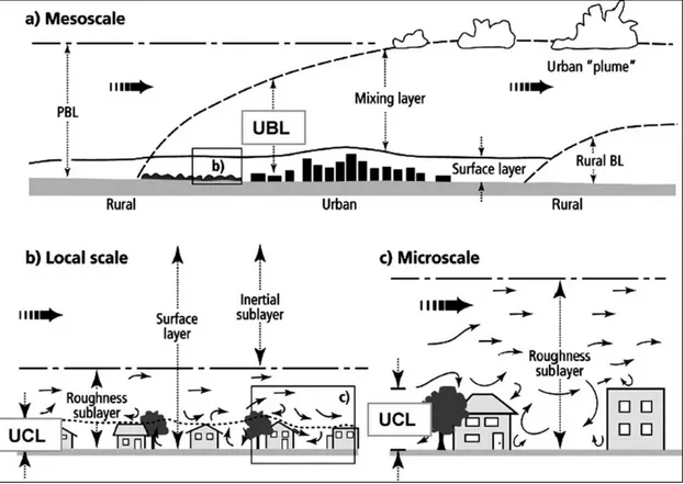
2.1 Buildings effect on airflow over different spatial scales. From http://uhiprecip.yolasite.com/. 17 2.2 Comparison of land-surface heat exchanges between urban and rural

areas. From http://uhiprecip.yolasite.com/. . . . 19 2.3 Schematic resume of the most relevant factors which contribute to the

generation of the UHI [Rizwan et al., 2008]. . . 20 3.1 The local climate zone (LCZ) classification scheme and its 17 standard

classes. From [Stewart and Oke, 2012]. . . 29 3.2 Digitized training areas for the study area considered. . . 30 3.3 Urban morphology defined through WUDAPT; classes from 1 to 10 are

urban type, while the others from A to G are rural/water types. . . 31 3.4 Urban morphology for the mesoscale model projected into Google Earth

map. Each pixel has a resolution of 500 m. Cyan pixels identify LCZ 3, green pixels LCZ 5, yellow pixels LCZ 6 and orange pixels LCZ 8. . . 32 3.5 Comparison between WUDAPT grid (opaque) and WRF grid

(transpar-ent) for the city of Bologna. The larger spread of the coarser one even in rural areas is evident. . . 33 3.6 Representation of the urban grid (dashed lines) and mesoscale grid (solid

lines). i ub and i ue are the first and the last urban levels within the mesoscale level I (from [Martilli et al., 2002]). . . . 38 3.7 Representation of the typical turbulent length scales within the urban

canopy from [Martilli et al., 2002]. . . 41 3.8 Schematic diagram of the energy balance of the solar panel and its

im-pact on radiation received by the roof. From [Masson et al., 2014] . . . 47 4.1 Daily minimum, mean and maximum 2-meter temperature for the month

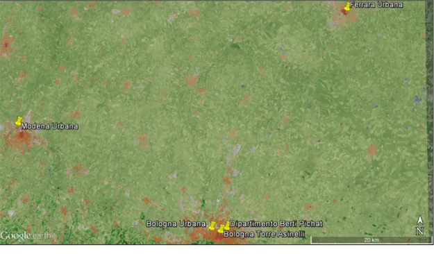
of July 2015. Data come from a weather station situated in the urban area of Bologna. . . 53 4.2 Rural stations within the finest grid.WUDAPT landmask has been

(8)

4.3 Hill stations within the finest grid. WUDAPT landmask has been over-layed. . . 57 4.4 Urban stations within the finest grid, for all the city (top) and with a

focus on the city of Bologna (bottom). WUDAPT landmask has been overlayed for the upper figure. . . 58 4.5 WRF 5-nested domains projected into Google Earth. . . 60 4.6 Schematic representation of the WRF Preprocessing System . . . 61 5.1 24-hour averaged values of 2-m air temperature,10-m wind direction,

wind speed and relative humidity registered by the Bologna Urbana weather station. Average have been computed for all variables from 6:00 to 5:00 of the next day. . . 68 5.2 Temperature time series of Observational data (blue dot), URB _NEST

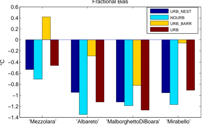
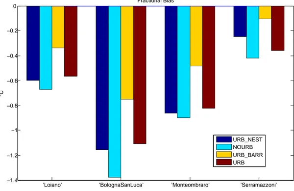
(red line) and NOURB(black line) for four different rural weather sta-tions. All the period of simulation have been taken into account (ne-glecting the spin-up period).The value in the x-axis refers to the 00:00 of each day. . . 71 5.3 Temperature Mean Bias between OBS and URB_NEST (blue bars), NOURB

(cyan bars), URB_BARR (yellow bars) and URB (red bars) for the four rural weather stations considered. . . 72 5.4 Temperature RMSE between OBS and URB_NEST (blue bars), NOURB

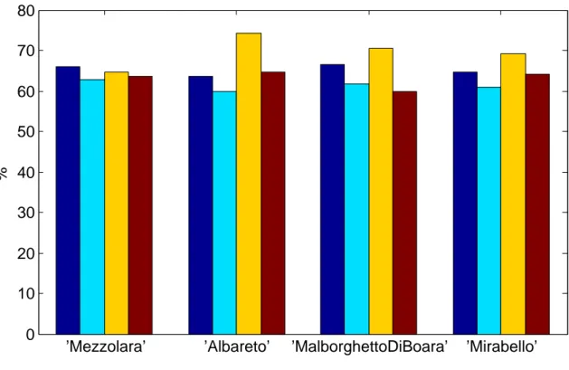
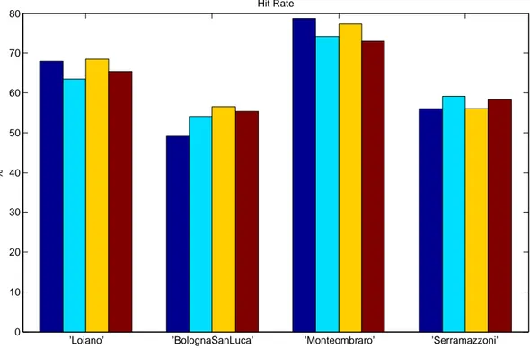
(cyan bars), URB_BARR (yellow bars) and URB (red bars) for the four rural weather stations considered. . . 72 5.5 Temperature Hit Rate between OBS and URB_NEST (blue bars), NOURB

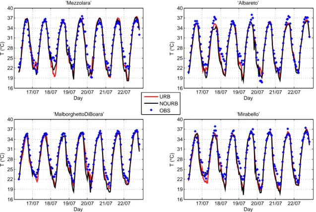
(cyan bars), URB_BARR (yellow bars) and URB (red bars) for the four rural weather stations considered. . . 73 5.6 Temperature time series of OBS (blue dot), URB _NEST (red line) and

NOURB(black line) for four different hill weather stations. All the pe-riod of simulation have been taken into account (neglecting the spin-up period).The value in the x-axis refers to the 00:00 of each day. . . 74 5.7 Temperature Mean Bias between OBS and URB_NEST (blue bars), NOURB

(cyan bars), URB_BARR (yellow bars) and URB (red bars) for the four hill weather stations considered. . . 74 5.8 Temperature RMSE between OBS and URB_NEST (blue bars), NOURB

(cyan bars), URB_BARR (yellow bars) and URB (red bars) for the four hill weather stations considered. . . 75

(9)

5.9 Temperature Hit Rate between OBS and URB_NEST (blue bars), NOURB (cyan bars), URB_BARR (yellow bars) and URB (red bars) for the four hill weather stations considered. . . 75 5.10 Diurnal Cycle of air Temperature for URB simulation and Observational

data in corrispondance of the weather station "Bologna Urbana". Er-rorbars are calculated between mean temperature and temperture of each day. . . 77 5.11 Temperature time series of OBS (blue dot), URB _NEST (red line) and

NOURB(black line) for five different urban weather stations. All the pe-riod of simulation have been taken into account (neglecting the spin-up period).The value in the x-axis refers to the 00:00 of each day. . . 78 5.12 Temperature Mean Bias between OBS and URB_NEST (blue bars), NOURB

(cyan bars), URB_BARR (yellow bars) and URB (red bars) for the four urban weather stations considered. . . 79 5.13 Temperature RMSE between OBS and URB_NEST (blue bars), NOURB

(cyan bars), URB_BARR (yellow bars) and URB (red bars) for the four urban weather stations considered. . . 79 5.14 Temperature Hit Rate between OBS and URB_NEST (blue bars), NOURB

(cyan bars), URB_BARR (yellow bars) and URB (red bars) for the four urban weather stations considered. . . 80 5.15 Relative Humidity time series of OBS (blue dot), URB_NEST (red line)

and NOURB (black line) for six different weather stations. All the period of simulation have been taken into account (neglecting the spin-up pe-riod).The value in the x-axis refers to the 00:00 of each day. . . 81 5.16 Relative Humidity Mean Bias between OBS and URB_NEST (blue bars),

NOURB (cyan bars), URB_BARR (yellow bars) and URB (red bars) for the four rural weather stations considered. . . 82 5.17 Relative Humidity Root Mean Squared Error between OBS and URB_NEST

(blue bars), NOURB (cyan bars), URB_BARR (yellow bars) and URB (red bars) for the four rural weather stations considered. . . 82 5.18 Diurnal cycle of wind for OBS and URB simulations. The black arrow

on the top-right side of the picture refers to the North direction. . . 84 5.19 Time series of wind velocity for "Loiano", "Bologna Torre Asinelli" and

"Settefonti" stations. . . 85 5.20 Time series of wind direction for "Bologna Urbana", "Bologna Torre

Asinelli" and "Settefonti" stations. In ordinate the direction of the in-coming wind. . . 86

(10)

5.21 Wind velocity Mean Bias between Observational data and URB_NEST (blue bars), NOURB (cyan bars), URB_BARR (yellow bars) and URB (red bars) for the three weather stations considered. . . 87 5.22 Wind velocity RMSE between OBS and URB_NEST (blue bars), NOURB

(cyan bars), URB_BARR (yellow bars) and URB (red bars) for the three weather stations considered. . . 88 5.23 Wind DIRECTION RMSE between OBS and URB_NEST (blue bars), NOURB

(cyan bars), URB_BARR (yellow bars) and URB (red bars) for the three weather stations considered. . . 89 5.24 Diurnal cycle of temperature difference between the stations "Bologna

Urbana" (urban) and "Mezzolara" (rural) for URB (red solid line), NOURB (green solid line) and OBS ( blue dashed line). Errorbars represent the RMSE relative to the mean difference. . . 90 5.25 Diurnal cycle of temperature difference between the stations

"Sette-fonti" (hill) and "Mezzolara" (rural) for URB (red solid line), NOURB (green solid line) and OBS ( blue dashed line). Errorbars represent the RMSE relative to the mean difference. . . 91 5.26 Diurnal cycle of temperature difference between the stations "Modena

Urbana" (urban) and "Albareto" (rural) for URB (red solid line), NOURB (green solid line) and OBS ( blue dashed line). Errorbars represent the RMSE relative to the mean difference. . . 92 6.1 Map of 2-meter air temperature of URB averaged over six 24-hour

pe-riod (fromt 6:00 of the first day to the 6:00 of the last day, i.e. from the 11t h hour until the 155t h hour). In the same way, 10-meter wind vec-tors averaged over the same period have been overlayed. The map also shows the contours of terrain height (plotted every 50 m) and urban morphology. . . 96 6.2 Map of 2-meter air temperature difference (URB-NOURB) averaged over

six 24-hour period (fromt 6:00 of the first day to the 6:00 of the last day, i.e. from the 11t hhour until the 155t hhour). . . 97 6.3 Map of 2-meter temperature and wind vectors (URB simulation) at 10:00

averaged over all the 6 days of simulation at the same hour. . . 98 6.4 Map of 2-meter temperature and wind vectors (URB simulation) at 14:00

averaged over all the 6 days of simulation at the same hour. . . 98 6.5 Map of 2-meter temperature and wind vectors (URB simulation) at 18:00

(11)

6.6 Map of 2-meter temperature and wind vectors (URB simulation) at 22:00 averaged over all the 6 days of simulation at the same hour. . . 100 6.7 Map of 2-meter temperature and wind vectors (URB NEST simulation)

at 2:00 averaged over all the 6 days of simulation at the same hour. . . . 100 6.8 Map of 2-meter temperature and wind vectors (URB simulation) at 6:00

averaged over all the 6 days of simulation at the same hour. . . 101 6.9 Diurnal cycle or sensible heat for the city of Bologna (Red Line) and a

closer rural cell on the northern side of the city (Green Line) for URB simulation. Sensible heat assumes positive values when the heat is re-leased from the surface to the atmosphere, and vice versa for negative values. Error bars are the MRSE calculated from the bias of each day. . 101 6.10 Representation of the vertical section used here projected on the map

for the city of Bologna. . . 102 6.11 Time series of the PBL height for a urban grid (x=120,y=70) and for a

rural one (x=120,y=110) for all the time of simulation. The simulation considered is URB_NEST. . . 103 6.12 TKE vertical plots for a urban grid cell (x=120,y=70) and for a rural one

(x=120,y=110). The TKE has been computed for the time period (00:00-21:00) of the 18th of July with a time interval of 3 hours. . . 104 6.13 Potential Temperature vertical plots for a urban grid cell (x=120,y=70)

and for a rural one (x=120,y=110). The TKE has been computed for the time period (00:00-21:00) of the 18th of July with a time interval of 3 hours.105 6.14 Vertical section of potential temperature,centered in Bologna, at 02:00

of the third day of simulation. The PBL is stable in rural zones, but un-stable over the city. The sections refer to URB (top) and NOURB (bot-tom) simulations. . . 106 6.15 Vertical section of potential temperature,centered in Bologna, at 16:00

of the third day of simulation. The PBL is unstable along all the longi-tude. The sections refer to URB (top) and NOURB (bottom) simulations. 107 6.16 Diurnal cycle of 2-m temperature differences (top) and PBL height

dif-ferences (bottom) averaged for the entire 6-day time period and across all urban cells of Bologna for all coverage rates of RPVP. Differences have been computed subtracting the URB simulation too all the PF_fraction simulations. . . 108

(12)

6.17 Diurnal cycle of skin temperature differences averaged for the entire 6-day time period and across all urban cells of Bologna for all coverage rates of RPVP. Differences have been computed subtracting the URB simulation too all the PF_fraction simulations. . . . 110 6.18 2-m air temperature differences (URB-PV_1.00) during nighttime (top)

and daytime (bottom) for the city of Bologna. Nightly average have been performed from 20:00 to 2:00, while daily average from 9:00 to 15:00 for each day of simulation. . . 111 6.19 PBL height differences (URB-PV_1.00) during nighttime (top) and

day-time (bottom) for the city of Bologna. Nightly average have been per-formed from 20:00 to 2:00, while daily average from 9:00 to 15:00 for each day of simulation. . . 113 6.20 Diurnal cycle of energy production by RPVP (left) and energy

consump-tion by ACS (right) for the URB simulaconsump-tion and all simulaconsump-tions with RPVP. Data have been averages over all days of simulation and over all urban grid cells of the city of Bologna. Unity of measurement refers to the power per unit of roof area. . . 114 6.21 Diurnal cycle of difference between energy production by RPVP and

en-ergy consumption by ACS for the URB simulation and all simulations with RPVP. Data have been averaged over all days of simulation and over all urban grid cells of the city of Bologna. Unity of measurement refers to the power per unit of roof area. . . 115

(13)

List of Tables

3.1 Comparison between the urban coverage percentage between WUDAPT grid (100 m of resolution) and WRF grid (500 m of resolution). . . 33 3.2 Thermal coefficients and length scales for the buildings for each UCZ. 35 3.3 List of symbols used in BEM . . . 49 4.1 Number of stations which provide the

relative variable for each landuse category. . . 54 4.4 Features of the weather stations within the domain. In the first column

is reported the name of the station, in second and third the position within the mesoscale grid, in the fourth the altitude over the sea level and in the last two the real position in coordinates. . . 57 4.5 Features of the five domains. . . 59 4.6 List of simulations performed and its features . . . 65 6.1 Enrergy production/consumption budgets. In the second column the

percentage of energy consumption with respect to the case without RPVP is shown. In the third column, the percentage of energy produced with respect to the energy consumed is reported. Values refers to an entire diurnal cycle. . . 117

(14)

List of Abbreviations

PBL Planetary Boundary Layer

UBL Urban Boundary Layer

UHI Urban Heat Island

RSL Roughness Sublayer

ISL Inertial Sublayer

UCL Urban Canopy Layer

NWP Numerical Weather Prediction

WUDAPT World Urban Database Access Portal Tool

USEB Urban Surface Energy Balance

LCZ Local Climate Zone

BEP Building Effect Parametrization

BEM Building Energy Model

RPVP Rooftop PhotoVoltaic Panels

WRF Weather research and Forecasting (model)

WPS WRF Preprocessing System

2WN two-way nesting (method)

1WN one-way nesting (method)

RH Relative Humidity

PT Potential Temperature

TKE Turbulent Kinetic Energy

(15)

Chapter 1 Introduction

The Urban Heat Island (UHI) effect is a well-known phenomenon defined as the dif-ference of temperature between an urban area and the rural one.

The impact of urban structures have been studied for decades, and it is still subject of interest, since the urban world’s population keeps increasing.

Cities have deep impacts on climate on different spatial scales: from microscale ( building and urban canyon) to mesoscale (city and surrounding areas) to macro-scale (regional and global). These impacts include the UHI, air quality, air pollution and CO2emissions. At the same time, the urban environment may affect health, en-ergy consumption and water supply.

Numerical Weather Prediction (NWP) modeling is considered an efficient tool for studying the effect of urban structures in a given environment; a wide range of suc-cessful applications is well-documented in scientific literature. Numerical modeling deals with different spatial scales: from microscale models (such as Computational Fluid-Dynamics (CFD) models), to single-building models (i.e the study of energy budget for a single structure), to mesoscale models (dealing with atmospheric struc-tures of the order of 10-100 km). A common task for all models is to reproduce ac-curately the features of urban morphology, with respect to the scale involved. Mi-croscale models require a detailed resolution of urban structures. On the other hand, models with coarser resolution need a parametrization of averaged urban morphol-ogy features for the spatial scales involved.

In particular, mesoscale atmospheric models have been widely used in the last years to study urban heat islands, using schemes representing the impact of urban envi-ronment within NWP models. The use of properly designed modeling systems pro-vides helpful information to civil protection and urban planning, in order to find mit-igation strategies able to contrast the harmful effects of urbanization.

(16)

Defining the urban coverage at suitable scales as input for the models is not a trivial task. Moreover, information of urban morphology has been identified as crucial to improving modeling capacity.

The aim of this work is to evaluate the capability of a high-resolution digitized ur-ban landmask in reproducing the UHI effect during a strong heat wave in Emilia-Romagna region.

The urban landuse has been created through the World Urban Database Access Por-tal Tool (WUDAPT), which provided an urban classes categorization through satellite imaginery. The landmask created with WUDAPT has been thereafter incorporated in the Weather Research and Forecasting (WRF) Model (a next-generation mesoscale numerical weather prediction system), originally developed by the National Center of Atmospheric Research (US) in the last decade. The Building Effect Parametriza-tion [Martilli et al., 2002] and the Building Energy Model [Salamanca et al., 2010] have been coupled with WRF to take into account the created landmask. Once validated the model capacity, the deployment of Rooftop Photovoltaic Panels (RPVP) in con-trasting the potentially harmful effect of UHI have been evaluated (i.e. depending on the latitude of the city considered).

Despite the physics describing the urban micro-climate is universal, the lack of a general method for the definition of the urban texture (morphology) is an obstacle for the realization of a robust climatic model. The problem is relevant especially for the study area, where cities are small and spread, and need to be adequately resolved with high resolution landmasks. At the same time, despite building databases are available for the study area considered in this thesis, they are unsuited for the task and their coverage is focused just on largest cities. For these reasons, WUDAPT is the most appropriate tool for the aim of this study: its versatility allows to describe universally the urban morphology. Its resolution can resolve the urban structures at suitable scales for the model used.

An appropriate description of the urban morphology is also a strong skill for the eval-uation of mitigation strategies which can be applied in order to contrast the harmful effects of the UHI.

The current introduction chapter is followed by a general review of physical patterns commonly adopted to describe the Urban Bondary Layer (Chapter 2). The focus will be set on the phenomenon which lead to the formation of UHI. The subsequent

(17)

(Chapter 3) deals with the urban landmask adopted in this work and the parametriza-tions used to take into account of urban structures within the model. Then the fea-tures of the region and the period object of this study and the setup used for the numerical simulations will be presented (Chapter 4). Finally, the comparison with observational data (Chapter 5) and the evaluation of the simulation resuls (Chater 6) will be discussed.

(18)

(19)

Chapter 2 State of art: studying the urban climate

In this chapter, the most relevant features of the atmospheric Urban Boundary Layer and its features are described, with particular emphasis on the Urban Heat Island (UHI) effect. Furthermore, the possible mitigation strategies that could be adopted to improve the urban climate are illustrated as well as the state-of-art models employed to numerically analyze this phenomena.

2.1 The influence of the cities on the near surface

atmo-sphere

In a review of United Nations in 2014, it was estimated that 54 % of the world’ s pop-ulation resided in urban areas in 2014. In 1950, 30 % of the world’ s poppop-ulation was urban, and by 2050, 66 % of the world’ s population is projected to be urban [Na-tions, 2014]. In particular, the percentage of urban population in Italy is currently of 69% [data.worldbank.org]. This means that the urban environment has become the most common ecosystem for humankind, and this phenomena keeps growing. Moreover, urbanization is one of the main anthropogenic processes responsible for big changes in atmospheric and land surface heat exchange process. Studying and modeling the processes which occurs in this contest is become a crucial point in or-der to improve the standard of living in urban areas, due to the strong impacts of cities on climate on a wide range of spatial scales. Cities environment has significant implications on local climate: temperature, precipitation, humidity, wind and radi-ation balances show noticeably differences between a city and its surrounding rural areas [Stewart, 2011]. Urbanization has also several implications on human heat re-lease and energy consumption: due to the city influence of on the local climate air pollution, anthropogenic heat increased release and negative influences on human

(20)

health are problems commonly found in this context.

2.2 The urban boundary layer

The planetary boundary layer (PBL) is the lowest part of the troposphere, influenced by the processes which take place in the planetary surface. It usually responds to the surface radiative forcing in a time scale of one hour, and it is generally turbulent and with a strong vertical mixing. Above the PBL lies the part of atmosphere not in-fluenced by the surface. Here the wind is geostrophic, i.e. it follows approximately the isobars, and it is usually nonturbolent. The Urban Boundary Layer (UBL) is the part of the atmosphere in which most of the humankind lives, and is one of the most complex microclimate due to its heterogeneity. We now report on the typical charac-teristic of the UBL, following the review of [Barlow, 2014].

Scales Involved: It is possible to characterize the UBL based on the scales of the

urban morphology. Therefore, the smaller one is the street scale (' 10−100m) where flows are influenced by each individual building. At the neighborhood scale (' 100 − 1000m) the atmosphere is influenced by average buildings with height, shape, and density. Finally, the city scale (' 10−20km) which corresponds to the dimension of city.

Energy Balance: The energy balance within the city is generally different from the

balance which takes place on the rural areas, because of the following reasons: • Sensible heat flux is higher because of buildings materials and increased

occu-pied area;

• The lower fraction of vegetative coverage reduces the latent heat flux;

• High thermal inertia due to the high heat capacity of the building materials, with a great storage within walls, roofs and ground;

• Shadowing and radiation trapping effect within the urban canyons. It affects the global albedo and the net long-wave radiation flux;

• Contribution of the anthropogenic heat release to the solar-driven energy bal-ance, which globally increases the sensible heat flux.

The increased sensible heat flux released strongly affects the vertical structure and then the height of the UBL.

(21)

Figure 2.1: Buildings effect on airflow over different spatial scales. From http://uhiprecip.yolasite.com/.

The different types of UBL The PBL flow is strongly influenced by surface

hetero-geneities. In fact, heterogeneities enhance the transfer of kinetic energy from the mean flow into turbulent flow, diminishing the velocity of the mean flow. The rough-ness of the ground is a relevant variable which affect the turbulent kinetic energy (TKE) production. In the urban context, roughness elements are significantly large, and exert a relevant drag on the flow. It is possible to classify two different roughness layers:

• The urban roughness sublayer (RSL), which has a depth of 2 − 5H, where H is the mean building height. Here the flow is high spatially dependent and domi-nated by turbulence;

• The inertial sub-layer (ISL), above the RSL, where turbulence is homogeneous and not dependent on the height.

Over the ISL, it is assumed that the UBL has the features of a classical PBL. In particular, during night-time, the positive sensible heat flux drives a nocturnal mixed layer which can be convective or near-neutral. Fig.2.1 represent these different layers.

(22)

Larger Scales features: As said before, the UBL structure is driven by the

ur-ban surface features, but this is not the only factor. At larger scales (10 −100km) thermal circulations can affect the UBL behavior. For example, coastal cities are subject to sea/land breezes due to land-sea temperature gradients. There-fore, the katabatic/anabatic wind can interact with the thermal circulation of the cities at the feet of the mountains.

2.2.1 The urban surface energy balance

Here the components of the urban surface energy balance (USEB) from [Arnfield, 2003] are reported. For a given volume within the urban canopy, the balance is:

Q∗+QF= QH+QE+ ∆QS+ ∆QA

Where:

• Q∗is the net radiation;

• QF is the anthropogenic heat flux;

• QHis the sensible heat flux;

• QE is the latent heat flux;

• ∆QSis the storage heat flux;

• ∆QAis the advective heat flux;

The storage flux The storage flux is due to the heat stored within the buildings

ma-terial. In order to correctly simulate the USEB, understanding the storage heat flux is of fundamental importance. It is subject to a large uncertainty, due to the variety of materials with different thermal properties present in a city. Moreover, it is not possible to measure it directly, but only through heat flux differences. It is strongly dependent on solar variation and on the buildings material features.

The anthropogenic flux Of fundamental importance is to be able to simulate the

interaction between anthropogenic flux and urban canopy air temperature, e.g. if the temperature is higher, the increase of the air conditioning to maintain constant the temperature inside the building leads to a greater anthropogenic flux. Numerical simulations shows that the impact of the anthropogenic heat flux on the UBL leads to a temperature increase of O(1◦C) and a consequent increase of the TKE, strongly

(23)

Figure 2.2: Comparison of land-surface heat exchanges between urban and rural areas. From http://uhiprecip.yolasite.com/.

dependent on the density of buildings. [De Munck et al., 2013] shows that larger in-creases were seen during nighttime, despite larger anthropogenic release during the day. This is due to the lower UBL height during night: the mixing of heat takes place in a shallower layer, leading to a temperature increase.

2.2.2 The nocturnal UBL

The nocturnal UBL differs from the day-time UBL, due basically to the absence of the solar radiation forcing; it is possible to outlining the following relevant features:

• In absence of a synoptical wind forcing, a positive heat flux can be maintained after the inversion of the net radiation; the urban surface cools less rapidly than the air above, leading to a convective turbulent layer within the UCL, princi-pally due to the heat stored inside the buildings materials. This convection decays gradually with the surface cooling i.e. with the heat dispersion through the upper and lateral layers.

• In a synoptical forcing condition, cooler rural air could advects over the warmer urban surface, leading to a positive surface heat flux from the surface to the in-coming air. This phenomena can form a near neutral layer close to the surface,

(24)

with a strong inversion on the upper ones, due to the mixing of warmer air. This thermal layer is identified as "thermal plume".

• In cities close or in the mountains, orography can trigger downslope cool flows, leading to stable layers over the city.

• Coastal cities strongly influence the sea breeze: the breezes could be main-tained during the night due to the increased land-sea temperature horizontal gradient, leading to weak convection caused by the cold air advection.

2.3 The urban heat island

The most relevant variable which could better distinguish rural and urban climates is the air temperature: on average cities are warmer than their rural surroundings, and this is the so called Urban Heat Island (UHI) effect, identified as the air temperature difference between the city the close rural areas. The principal causes that lead to this phenomena are related to the urban thermal, moisture, aerodynamic and radiation features, different from the rural ones. These differences are mainly linked to the presence of buildings, which are built with materials of low permeability and high heat capacity. In addition to the urban structures (and then radiation trapping within urban canyons), pollutant emissions and anthropogenic heat release contribute to warm the urban environment.

Figure 2.3: Schematic resume of the most relevant factors which contribute to the generation

(25)

The air temperature difference caused by the UHI effect has a diurnal and sea-sonal variability: several studies stated that this phenomena is greater during sum-mer due to the higher incoming solar radiation with respect to winter, and stronger during night-time, because of the heat storage within the urban structures [Charabi and Bakhit, 2011]. For the largest cities, it is also possible to identify temperature variabilities within the same city: the greatest differences have been noticed between high residential and vegetated zones. Green areas within urban environment highly contribute in decreasing UHI effect [Arnfield, 2003]. The intensity of the effect is also related to the synoptical conditions: [Rizwan et al., 2008] reported that anticyclone conditions increase the effect, while increasing wind speed and cloud coverage can diminish the harmful effects due to the urban land use. [Tran et al., 2006] showed the positive correlation between UHI and city population. The population and its den-sity could have both direct and indirect effect on the UHI: increasing the number of people, anthropogenic release grows, and on the other hand a wider building cover-age is requested in order to host all the people living in cities. UHI may have harmful effects on urban population especially those located at lower latitudes. The thermal discomfort causes cardiovascular and respiratory problems to the citizens, in partic-ular heat-related illness and fatalities, such as heatstrokes, heat exhaustion, heat syn-cope especially in the elderly and children. In the same way, respiratory problems are related to the high ozone percentage within the city induced by heat wave events and traffic emissions. A study conducted by [Heaviside et al., 2015] in the West Midlands (UK), suggests that UHI effect contributed around 50% of the total heat-related mor-tality during the 2003 heatwave. This phenomena will be 3 times stronger in 2080, due to the change in population, population weighting, weather conditions and as-suming no change in anthropogenic heat release.

2.3.1 Mitigation strategies to reduce the UHI

It is important to outline the effects and causes of the UHI, in order to find contrasting methods able to reduce the dangerous effect of this phenomena. [Gago et al., 2013] resumes the features of the urban micro-climate into four relevant points:

• A temperature increase with respect to the rural areas; • A reduction in the daily temperature range;

• A modified wind distribution within the city due to the friction with buildings; • A water budget that differs from the rural one.

(26)

Principal Causes of the UHI effect

Urban Geometry • Proprieties of urban materials • Radiation Trapping within urban canyons

• Building-induced turbulence • Reduced green areas, i.e reduced evapotranspiration

Anthropogenic Heat Release • Air conditioning systems • Vehicular circulation

Synoptic Conditions • Heat wave periods • Clear sky and calm wind • Proximity to large water bodies and mountainous terrain

Since modification of urban features cannot take place on large scales (often the city are old or big, then a radical modification of the geometry is too difficult to act), it is necessary to identify the most important elements which affect urban temper-ature on local scale. Mitigation strategies need to be focused on the following fea-tures [Wong et al., 2011]: buildings, green spaces and pavements. Therefore, it is possible to set some parameters in order to evaluate the influence of the previous three elements on the urban environment:

• green areas ratio; • sky view faction; • building density; • wall surface area; • pavement area; • albedo.

Mitigation strategies concentrate on the modification of the previous parame-ters, in order to change the heat surface balance and consequently reduce the UHI effect. Green roofs, cold pavements and green spaces in urban areas are all measures that are helpful to reduce the surface temperature, heat absorption and energy con-sumption. In fact, evapotranspiration plays a key role in cooling urban surfaces: the process consists in the release of vapor by vegetation forced by solar radiation, that

(27)

spread on the surrounding areas [Bowler et al., 2010]. Due to this phenomena, the heat stored within urban materials can diminish. Finally, the research on the mitiga-tion strategies could be lead looking at the effect produced by the following elements:

• green areas and roofs; • trees and vegetation; • pavement;

• albedo.

Green areas and roofs: The combined effect of evapotranspiration and shading

sig-nificantly decreases air temperature, and leads to the formation of cool island in the city, and could reflect their beneficial effects on the surrounding areas. Furthermore, it was found that green spaces reduce the temperature changes produced by build-ing materials. The same effect is caused by green roof; the displacement of vegetation over the buildings can improve building energy performance as well as the environ-mental conditions of the surroundings. The second effect of green areas within the city is the deposition: pollutant are retained by vegetation.

Trees and vegetation: [Robitu et al., 2006] showed that 10% of the energy consumed

in cooling building can be saved through the temperature reduction caused by veg-etation. On the other hand, vegetation displacement in the urban context can neg-ative affect the local microclimate in cold climates: in this case vegetation shading and radiation absorption increase heating costs up to 21%.

Pavement: The most relevant aspect of urban pavement which affect the local

cli-mate are the horizontal surface exposed to solar radiation, albedo and the thermal capacity. For that reason, in order to reduce the solar radiation absorbed by pave-ment, the use of smooth, light-colored and flat surfaces tend to be more efficient in reducing the heating effect.

Albedo: Albedo play a key role on the urban radiation budget: the incident solar

radiation in absorbed and transformed into sensible heat (stored in building mate-rial and released in the atmosphere), which contribute in heating the urban envi-ronment. [Salamanca et al., 2016] analyzed the impact of the displacement of high-albedo roofs and rooftop photovoltaic panels (RPVP). This study demonstrates that the deployment of cool roofs and RPVP reduce both near-surface air temperature and cooling energy demand across all the diurnal cycle.

(28)

2.4 Models used to investigate the UHI

The study of this phenomenon could involve different spatial scales, with respect to the aim of study [Mirzaei, 2015]. Therefore, different resolutions are required to investigate the most relevant aspects. In the following paragraph a description of the models used to investigate the UHI effect is shown.

Microscale models: The basis of the development of microclimate models is the

interaction between a building and its surrounding environment. These models in-clude solar radiation and surface convection induced by buildings’ surfaces. Gen-erally the airflow features are resolved using computational fluid dynamics (CFD) models, with a grid resolution of the order of 1 meter. These models can take into account the effect of different parameters such as building features and vegetation on the surface induced convection, human health and urban ventilation. Moreover, microscale models can deal with the effect of pollutant and its diffusion within urban morphology’s heterogeneities.

Building-scale models: These models deal with the energy balance for an isolated

building, not taking into account the effect of the surrounding ones. The effect of the building and its energy balances (such as urban environment, ventilation, heat exchange through the walls) on the outdoor parameters could be computed. Often these kinds of model are integrated within larger scale models (such as in this current work).

Mesoscale models: These kinds of model deal with the large-scale variation of the

UHI effect. Urban-scale features, urban ventilation, pollution dispersion, anthro-pogenic release balance and mitigation strategies could be investigated through the use of mesoscale models. They can capture the synoptic features of the region of interest and at the same time provide informations about local-scale phenomenon. Often a coupling with coarser or finer scale model is used, in order to better describe variabilities and the balances which take place within the urban environment.

Summary

In this chapter, the most relevant general features of the topic investigated in this work are presented.

Starting from explaining why it is important to study the harmful features of the UHI effect, we have the characteristics of the Urban Boundary Layer (UBL), which is the

(29)

part of the Planetary Boundary Layer influenced by urban morphology. UBL has been described focusing on:

• The different spatial scales involved (from street scale to the city scale), and the different types of UBL;

• The energy balance: it is substantially different from the energy balance taking place on rural areas, since buildings heat storage plays a key role in the heat balances;

• The nocturnal UBL: during nighttime, the UBL shows the highest differences with respect to rural areas, since a positive heat flux can be maintained.

Furthermore, the processes which lead to the UHI effect have been discussed: the UHI is principally caused by geometry and composition of urban structures, anthro-pogenic heat release and absence of synoptic forcing.

Several mitigation strategies can be adopted in order to contrast the harmful conse-quences induced by the UHI. They concern the increase of urban vegetation and the modification of the value of albedo for urban surfaces.

Finally, in order to introduce further development addressed in this thesis, the most used models commonly adopted to study the UHI have been discussed. Basically, they differ one from another for the spatial scale of interest: microscale models are used to investigate the building and street scale, building-scale models to study the interaction between a building and its surrounding area while mesoscale models to evaluate large-scale variation.

(30)

(31)

Chapter 3 Outlining the urban morphology

In the first part of this chapter, the method used to define the urban coverage within the region of interest is presented. Several methods can be used: in this work, satel-lite data have been combined with built digitized data in order to provide an effi-cient landmask. Moreover, the second part deals with the parametrizations which have been coupled with WRF to take into account the effect of buildings within the UCL: the Building Effect Parametrization [Martilli et al., 2002] and the Building En-ergy Model [Salamanca et al., 2010].

3.1 Parametrization of the urban morphology

One of the crucial points of the UHI modeling, is the definition of the urban features within the domain of the simulation: information on urban morphology has been identified as critical to improve modeling capacity [Masson, 2006], [Stewart et al., 2014], [Chen et al., 2011].

Moreover, since the mesoscale model has a finest resolution of 500 m, it is neces-sary to identify for each grid cell averaged values describing coherently the features of the buildings. Therefore, parametrizing the urban morphology is not a trivial task. In addition, another problem is linked to the lack of real data to be used within the model. The urban landscape can be created assembling from several sources, such as land-use/cover maps, building databases and satellite/lidar data [Brousse et al., 2016]. In this work, the use of satellite data has been chosen, and the urban morphol-ogy has been parametrized through the recently developed World Urban Database Access Portal Tool (WUDAPT) software (with a spatial resolution of 100 m), and later interpolated into the mesoscale model grid (with a spatial resolution of 500 m).

(32)

3.2 The WUDAPT software

3.2.1 Creating the urban landmask with WUDAPT

In order to identify a correct parametrization for the urban morphology, the World Urban Database Access Portal Tool (WUDAPT) has been used [Bechtel and Daneke, 2012], [Stewart and Oke, 2012], [Bechtel et al., 2015]. WUDAPT allows to classify ur-ban structures into 17 different classes (Local Climate Zones,LCZ), ten of which are urban, and other seven rural (not considered in WRF landuse classification). The prototype of each class ais reported in Fig. 3.1.

At each urban climate zone (UCZ) are associated several variables (thermal coef-ficients, building length scales, height distribution and vegetative covering ratio) that can be chosen within a range of values established empirically. In order to capture the correct urban coverage to be implemented in the model, the following process has to be followed, as reported in WUDAPT’s guide (www.wudapt.org):

• Creation of the LCZ training areas: Through the use of Google Earth Pro, LCZ polygons have been manually built for each class within the study area. This process is necessary in order to make a comparison between training areas and satellite data. Several zones are requested to represent truly the diversity of urban landscape. This process is characterizing correct landscape using pho-tographs describing the typical land cover and building prototype associated with each LCZ. The training areas used in this work are shown is Fig. 3.2; • Comparison with satellite data: Training areas need to be compared with

satel-lite data.In order to distinguish between the different urban classes, three clear-sky and cloudless days Landstat8 satellite images (with a spatial resolution of 100 m) have been used in SAGA GIS software [Conrad et al., 2015]. Nine images per day have been chosen, each one representing a different wave length of the radiation reflected by the surface .

In particular the days chosen for this work are the 18/03/213, the 16/07/2013 and the 10/06/2014: it is important to use data for several days, in order to avoid systematic errors due to a single-day analysis. SAGA GIS automatically classify the pixels in the region of interest into LCZ types, superimposing the training area scenes to the satellite data. In other words, SAGA GIS is able to detect the different features within the study area (from the satellite data), and assign to the pixels not covered with the training polygons the correct LCZ type; • Iteration process: Once created the first raw classification, the LCZ map has been compared with the underlying Google Earth landscape; this is useful to

(33)

Figure 3.1: The local climate zone (LCZ) classification scheme and its 17 standard classes.

(34)

Figure 3.2: Digitized training areas for the study area considered.

refine the LCZ classification, until the comparison with the real data map will result satisfactory.

The resulting map for the study area considered (including the urban zones of Bologna, Modena, Ferrara, Reggio Emilia, Sassuolo and Imola) is shown in Fig. 3.3. The urban coverage built with WUDAPT shows that the urban coverage is 684.73 km2; 0.93% is Compact Mid-rise (LCZ 2), 26.00% Open Mid-Rise (LCZ 5), 35.32% Open Low-Rise (LCZ 6) and 37.09% Large Low-Rise (LCZ 8). This means that there are not areas clas-sified as Compact High-Rise (LCZ 1), Compact Low-rise (LCZ 3), Open High-rise (LCZ 4), Lightweight Low-Rise (LCZ 7) and Heavy Industry (LCZ 10).

3.2.2 Including the LCZ map into WRF

The next step, is to include the resulting urban coverage within the finest domain of the model: since the grid resolution of the WUDAPT grid is 100 m, and that one of the WRF is 500 m, an interpolation method is requested. In fact, within the same model grid cell, there are several LCZ classes, and an averaged value for the grid cell need to be identified. Therefore, has been decided to choose the most present LCZ value within each cell (following the guide provided by [Martilli et al., 2016]). This means that, for the calculation of the atmospheric parameters, the mesoscale model will consider the values belonging to the LCZ with the high coverage rate in the grid cell considered. Fig.3.4 shows the resulting LCZ classification superimposed on the

(35)

Figure 3.3: Urban morphology defined through WUDAPT; classes from 1 to 10 are urban type,

while the others from A to G are rural/water types.

Google Earth map of the study area.

The final result, shows that the urban coverage is 400.25 km2; 1.2% is Compact Mid-rise (LCZ 2), 23.05% Open Mid-Rise (LCZ 5), 33.35% Open Low-Rise (LCZ 6) and 42.35 % Large Low-Rise (LCZ 8).

3.3 Comparison between WUDAPT and WRF urban

land-masks

The interpolation into the finest grid on the mesoscale 500 m leads to a loss of infor-mation. In this section, a comparison between the two landuse is performed.

In Tab. 3.1 the percentages of coverage of the different LCZ areas are shown. The value at the bottom of the table refers to the fraction of urban coverage with respect to the total surface of the domain. Results show an higher rate of coverage for the WUDAPT urban landscape (7.31% vs 4.78%): this a reasonable result, because

(36)

inter-Figure 3.4: Urban morphology for the mesoscale model projected into Google Earth map.

Each pixel has a resolution of 500 m. Cyan pixels identify LCZ 3, green pixels LCZ 5, yellow pixels LCZ 6 and orange pixels LCZ 8.

polating the WUDAPT grid into the coarse grid, small towns cannot be detected dur-ing interpolation. When the urban pixels are less dense, the interpolation through the most present value for each grid cell "chooses" a rural cell even though an urban one.

Checking class per class, LCZ 2 and LCZ 8 results most present in the mesoscale grid with respect to the finest one. Since in the domain considered city centers and in-dustrial areas are the most clustered in defined zones, they are easier to be detected by the interpolation, then their percentage of covering is higher in the coarser grid. On the other hand, LCZ 5 and LCZ 6 are more scattered and surrounded by rural areas than the first two, so the most present value within the mesoscale pixels is rural.

Focusing on the city of Bologna, the resulting urban landuse for the coarser grid often covers rural surround areas, better distinguished by the WUDAPT grid. As shown in Fig. 3.5, rural areas within the urban environment are not detected: since the most present value within each pixel of 500 m of resolution is always urban, all WRF cells for (and close) the city of Bologna have been detected as urban.

(37)

Urban Coverage Percentage WUDAPT (%) WRF (%) LCZ 2 0.93 1.2492 LCZ 5 26.66 23.05 LCZ 6 35.32 33.35 LCZ 8 37.09 42.35 Urban Coverage 7.31 4.78

Table 3.1: Comparison between the urban coverage percentage between WUDAPT grid (100

m of resolution) and WRF grid (500 m of resolution).

Figure 3.5: Comparison between WUDAPT grid (opaque) and WRF grid (transparent) for the

(38)

3.4 Definition of the urban parameters

After the classification of the urban coverage into LCZ, it is necessary to assign to each class its own parameters. The variables requested, different for each class are: fraction of urban landscapes which does not have vegetation, heat capacity, thermal conductivity, emissivity, roughness length and albedo for roof, ground and building wall, height distribution for the buildings (values are computed by steps of 5 meters), street and buildings width. Values used in this work are shown in Tab. 3.2. Since most of the parameters are not available for the study area, input data for the sim-ulations have been leaved as default. Variations with respect to default values con-cerns the thermal coefficients for the LCZ 2 and LCZ 5: the most employed material for roofs and walls is solid brick [Oke, 1987]. At the same time, given that most of ground is made of asphalt, also the characteristic values of this material has been set as input for the simulations. Finally, the last values which have been changed from the default setting are the height of the buildings: through the analysis of the height of building belonging to the city center (free data available on the website

www.dati.comune.bologna.it), and given that LCZ 2 and LCZ 5 assume on average

the same height, the mean percentage of buildings in the same range of height for each 5 meter level has been computed.

(39)

Table 3.2: Thermal coefficients and length scales for the buildings for each UCZ.

UCZ 2 UCZ 5 UCZ 6 UCZ 8

Urban Fraction 1 0.7 0.65 0.85

Roof Heat Capacity [_mJ3_K] 1.37 × 106 1.37 × 106 1.44 × 106 1.80 × 106

Roof Thermal Conductivity [_msKJ ] 0.83 0.83 1.00 1.25

Roof Albedo 0.20 0.20 0.20 0.20

Roof Emissivity 0.90 0.90 0.90 0.90

Roof Roughness Length [m] 0.01 0.01 0.01 0.01

Ground Heat Capacity [_mJ3_K] 1.94 × 106 1.94 × 106 1.47 × 106 1.80 × 106

Ground Thermal Conductivity [_msKJ ] 0.75 0.75 0.60 0.80

Ground Albedo 0.10 0.10 0.10 0.10

Ground Emissivity 0.95 0.95 0.95 0.95

Ground Roughness Length [m] 0.01 0.01 0.01 0.01

Wall Heat Capacity [_mJ3_K] 1.37 × 106 1.37 × 106 2.0 × 106 1.80 × 106

Wall Thermal Conductivity [_msKJ ] 0.83 0.83 1.25 1.25

Wall Albedo 0.20 0.20 0.20 0.20 Wall Emissivity 0.90 0.90 0.90 0.90 Road Width [m] 10 33.3 12.4 32.5 Buildings Width [m] 10 10 10.5 28.8 Buil. % with h < 5 m \ \ 40 35 Buil. % with 5 <h< 10 m 20 20 40 65 Buil. % with 10 <h< 15 m 30 30 20 \ Buil. % with 15 <h< 20 m 20 20 \ \ Buil. % with 20 <h< 25 m 20 20 \ \ Buil. % with 25 <h< 30 m 10 10 \ \

3.5 Parametrization of the effect of Urban Morphology

on near surface atmosphere

After the discussion on the methods used to parametrize the presence of buildings and urban structures within the study area, the main features used to take into ac-count the effect of the urban landmask on the atmospheric dynamics is presented. The two schemes used in this work are the Building Effect Parametrization (BEP) [Martilli et al., 2002] and the Building Energy Mode (BEM) [Salamanca et al., 2010]. While BEP takes into account the influence of buildings and urban heterogeneities on the UCL, BEM computes heat fluxes between the indoor and outdoor sides of each building. It also takes into account the presence of air conditioning systems (ACS),

(40)

windows and equipment inside the buildings’ rooms. In the next two sections these two schemes are discussed.

3.5.1 The BEP scheme

This multi-layer parametrization links the urban-scale phenomenon (10 m − 10km) with the meso-scale features (10 −100km), with the aim to compute the effect of the smaller scale on the mesoscale circulation. Since the horizontal dimensions of the domain are on the order of mesoscale, the horizontal grid resolution cannot be such detailed to resolve completely the urban heterogeneities. This leads to the fact that urban morphology effect on the PBL is not completely resolved, but need to be av-eraged with respect to the resolution of the model. Moreover, parameterizing such turbulent and complex flows, it is not possible to use the traditional constant-flux layer approximation through the Monin-Obukhov similarity theory within the RSL. Since the meso and the urban scales have different dimensions, but they exchange information each other, an average and interpolation process is necessary.

The mesoscale model

The following conservation equations represent the mesoscale features of the UBL dynamics. Capital letters denote Reynolds averaged variables, while small letters rep-resent the respective turbulent fluctuation (i. e. if ˜A is a variable, it can be seen as

˜

A = A + a, where A is the Reynolds averaged variable, and a0its respective fluctua-tion):

• Mass:

∂ρUi

∂xi = 0

Supposing the anelastic approximation. • Momentum: ∂ρUi ∂t = ∂P ∂xi + Fi with Fi= ∂ρUiUj ∂xj − ∂ρuiw ∂z − ρ θ0 θ0 gδi 3− 2εi j kΩj¡Uk−U_kG¢ + DUi

where the terms on the right hand side represent respectively the mean trans-port, the vertical turbulent transport (w refers to the vertical component of tur-bulent momentum flux), the buoyancy (θ0= θ − θ0, whereθ identifies the po-tential temperature) with the Boussinesq approximation, the Coriolis force (U_kG

(41)

is the k-component of the geostrophic wind), and the last term (DUi) resumes

all the forces induced by the interaction with the urban morphology. • Energy: ∂ρθ ∂t = ∂ρθUi ∂xi + Dθ− 1 Cp ³P₀ P ´_CpR ∂R_{l w} ∂z

where Cpis the specific heat at constant pressure, R the gas constant, P0the

ref-erence pressure and Rl w is the longwave radiation flux. Dθ takes into account

of the effect of urban surfaces on the potential temperature budget. • Air Humidity: ∂ρH ∂t = ∂ρHUi ∂xi − ∂ρwh ∂xi + DH

where H is the mean absolute humidity and h its turbulent fluctuation. Dh

takes into account of the effect of the latent heat from surfaces on the humidity balance.

The K-theory approach to parametrize the vertical fluxes is used. If A is the mean part of a given variable and a its turbulent component, the turbulent vertical transport is computed as:

w a = −Kz∂A

∂z

where Kzis the vertical diffusion coefficient. In order to calculate Kz, two

equa-tion are requested: one expressing the dependence of the diffusion equaequa-tion on the kinetic energy (E ) and length scale (lk), and a prognostic equation where

the dependence between E and lkis considered. These two equations are:

Kz= CklkE1/2 ∂ρE ∂t = − ∂ρUiE ∂xi −∂ρwe ∂z +ρKz(lk, E ) h ¡∂Ux ∂z ¢2 +¡ ∂Uy ∂z ¢2i −g θ0 ρKz∂θ ∂z−ρCε E3/2 l_ε +DE

where the third and fourth terms on the right hand side are respectively the shear and buoyant production terms, the fifth is the dissipation term and the last takes into account of the presence of the buildings. The first equation is the k − l closure scheme based on [Bougeault and Lacarrere, 1989]. lk and lε

are computed taking into account of the maximum distance that an air parcel can reach due to buoyancy effect up and down.

(42)

The Urban Model

As said before, BEP works with two different grids of different scales: the mesoscale and the urban-scale. They interact between each other, with the smaller one giving feedbacks to the coarser grid and vice versa. The urban scale grid used in BEP is able to represent within the mesocale grid the vertical features of the urban morphology, in order to take into account the sink of momentum and the source of heat fluxes due to the presence of buildings. However, this smaller grid is not able to represent exactly the urban morphology, so mean vertical and horizontal parameters for each cell are needed as input. These parameters are: street width (W ), building width (B ), mean height (h) and height probability distribution (γ(h)).

Figure 3.6: Representation of the urban grid (dashed lines) and mesoscale grid (solid lines). i ub and i ue are the first and the last urban levels within the mesoscale level I (from [Martilli et al., 2002]).

By now, it is important to take into account the interaction between the two grid, then the IU index refers to the urban grid, I to the mesoscale grid (at the same level of the horizontal face of the cell), while i u and i refers to the value in the center of the cell respectively for the urban and mesoscale grid. Now, the area fraction occupied by building for each vertical level zi u(over the ground) is computed, both for horizontal

and vertical direction:

S_{i u=1}H = W W + BS H t ot S_{i u>1}H = W W + Bγ(zi u)S H t ot

(43)

SV_IU= ∆zIU

W + BΓ(zi u+1)S

H t ot

where S_{t ot}H is the total horizontal surface of the grid cell, ∆zIU is the grid

spac-ing (could vary with the height) andΓ(z_{i u+1}) = nuP

j u=i uγ(zj u

) is the probability to have building higher of equal than z_{i u+1}. The computation could be performed for differ-ent direction, in order to take into account of the differdiffer-ent directions of the inciddiffer-ent wind. In our case, just the N-S and W-E directions are considered.

Effect of the Urban Morphology on the Airflow

In the equations for the mesoscale model, a DA term is added, in order to consider

the effect of buildings and urban surface on the airflow. The effects considered in this parametrization are:

• loss of momentum due to the drag induced by buildings;

• transformation of mean kinetic energy into turbulent kinetic energy; • shadowing and radiation trapping effects within urban canyons.

Turbulent Momentum Flux The turbulent momentum flux which originates due

to the drag of horizontal surfaces for each level i u is: ~FuH i u= −ρ k2 h l n¡∆z_IU 2z0i u ¢i2 fm( ∆zIU 2z0i u , RiB)|UIUH |~UIUSi uH

where U_IUH is the horizontal component of the wind, fm an empirical function

dependent from the bulk Richardson number computed at level IU (RiB=_T−g_IU_(Uz∆θHv IU)2

, whereθvis the virtual potential temperature), k is the Von Karman constant and z0i u is the roughness length at the level i u. The turbulent momentum flux due to the vertical surface is computed as:

~FuV

i u= −ρCd r ag|U V

IU|~UIUV SVIU

where ~U_IUV is the wind speed perpendicular to the vertical surfaces and Cd r ag is

the drag coefficient equal to 0.4 (computed from measurements in wind tunnel).

Turbulent Temperature Flux As in the computation of the momentum flux, the

(44)

Fθ_{i u}H = −ρ k 2 h l n¡∆zIU 2z0i u ¢i2 fh ³∆z_IU 2z0i u , RiB ´ |U_IUH|∆θS_{i u}H

where∆θ is the temperature difference between the horizontal surface and the air. For the vertical temperature it is not possible to use the previous equation, be-cause this kind of fluxes depends on the temperature differences between air and walls and on the street direction. Taking into account just of the N-S direction of the street the flux of sensible heat from walls is given by:

Fθ_{i u}V = − η Cp h ¡ θai r− θW E STIU ¢ + ¡θai r− θE ASTIU ¢i SV_IU

whereη is an empirical variable depending on the horizontal wind speed at the con-sidered level.

Turbulent Kinetic Energy Flux In the equation for the turbulent kinetic energy, a

parametrization for the buoyancy and shear therms is required. These terms are not computed as fluxes, because of the TKE is a volumetric variable. Multiplying the shear and buoyancy production terms for the volume of the respective grid cell, the resulting term is:

P r_{i u}H = · − ¡F u_{i u}H ρSH i u ¢3/2 k∆zIU 2 + g θ0 Fθ_{i u}H ρSH i u ¸ SH_{i u}∆zIUρ .

for the horizontal direction, while for the vertical direction:

F eV_IU= Cd r ag|UIUV |3SVIU

Computation of the urban morphology effect terms

Finally, one calculated the turbulent fluxes for momentum, temperature and kinetic energy, the inclusion of these terms into the equation is needed. The term reflecting the urban morphology effect are the DAterms appearing in the previous mesoscale

equations. Then, adding the vertical and horizontal terms and dividing for the vol-ume of the mesoscale grid cell, the resulting term is:

DAI =

F a_IH+ F aV_I

VI

where all the variables are calculated for the mesoscale grid, i.e. an averaging pro-cess for the urban scale grid cells within the same mesoscale grid cell is nepro-cessary.

(45)

Figure 3.7: Representation of the typical turbulent length scales within the urban canopy

from [Martilli et al., 2002].

In order to calculate numerically the vertical variation of the turbulent fluxes, the discretization of the mesoscale grid is used, but only for the cells not occupied by buildings: ∂ρwa ∂z = 1 V_IA(ρwaiS A i − ρw ai +1S A i +1)

Computation of the turbulent length scales

Within a urban parametrization, it is necessary to take into account of the effect of the buildings on the length scale. The lk and lε length scales are values required

to compute the turbulent kinetic energy dissipation term and the diffusion terms through the k − l closure (and the respective prognostic equation). The length scales parametrization presented here is a modification of that one proposed by Bougeault and Lacarrere (1989). In order to evaluate this parameter, as scale dimension of build-ing the height has been chosen. Since the buildbuild-ings does not have the same height within a grid cell, the following assumption is taken into account: while the lower levels can be influenced by building of all height, at higher levels the predominant vortices are induced by only the higher buildings. Finally, the length scale for a level

I is computed as: 1 l_{b I}= nu X i u=i bu γ(zi u) 1 zi u

where i bu is the lowest level of the urban cell within the considered mesocale cell, and nu is the highest level of the urban grid. This new length scale is added to