Reconstruction of non-prompt charmed baryon Λc with boosted decision trees technique

A

LMA

M

ATER

S

TUDIORUM

· U

NIVERSIT

A DI

`

B

OLOGNA

Scuola di Scienze

Dipartimento di Fisica e Astronomia Corso di Laurea in Fisica

Reconstruction of non-prompt charmed baryon Λ

_c

with Boosted Decision Trees technique

Relatore:

Prof. Andrea Alici

Presentata da:

Lorenzo Valente

Abstract

ALICE (A Large Ion Collider Experiment) is the heavy-ion experiment at the CERN Large Hadron Collider. It is focused to study the physics of strongly interacting matter at extreme energy densities when a transition occurs and a phase of matter called Quark Gluon Plasma (QGP) forms. In these conditions, the ALICE experiment investigates how the QGP expands and cools down. Due to its short average lifetime, the QGP cannot be studied directly. It can only be proved when the QGP cools down and releases the particles that constitute the matter. In this respect, the study of the so-called “ hard probes ” (hadrons containing charm or beauty quarks) represents an outstanding tool, since such particles are created in the early stages and are expected to lose a significant fraction of their energy when crossing the

decon-fined medium. The aim of this thesis is to reconstruct charmed Lambda baryon Λc and divide

non-prompt signal from prompt one, using Boosted Decision Trees technique. The analysis is performed using a multivariate analysis approach which allows to consider simultaneously multiple event properties, exploiting most of the available information through machine learn-ing techniques.

Contents

Introduction 4

1 Physics of the ALICE experiment 5

1.1 Introduction to the Standard Model . . . 5

1.2 Quantum ChromoDynamics . . . 7

1.2.1 Lattice Quantum Chromodynamics . . . 7

1.3 Quark-Gluon Plasma . . . 8 1.3.1 Phase transition of QCD . . . 8 1.4 Heavy-Ion Collisions . . . 10 1.4.1 Relativistic Kinematics . . . 10 1.4.2 Rapidity Variable . . . 10 1.4.3 Time evolution . . . 11 1.5 Experimental aspects . . . 12 1.5.1 Soft probes . . . 13 1.5.2 Hard probes . . . 15 1.5.3 Direct Photons . . . 18

2 The ALICE experiment 20 2.1 The Large Hadron Collider . . . 20

2.1.1 Magnetic lattice . . . 21

2.2 The ALICE experiment . . . 22

2.2.1 The ALICE detector . . . 22

2.2.2 Inner Tracking System . . . 24

2.2.3 Time Projection Chamber . . . 25

2.2.4 Transition Radiation Detector . . . 26

2.2.5 Time of flight . . . 27

2.2.6 High-Momentum Particle Identification Detector . . . 28

2.2.7 Calorimeters . . . 29

3 Reconstruction of non-prompt charmed baryon Λc with Boosted Decision Trees

technique 31

3.1 Introduction . . . 31

3.2 The Toolkit for Multivariate Data Analysis . . . 32

3.3 Boosted Decision Trees (BDT) . . . 33

3.3.1 Gradient Boost . . . 34

3.4 BDT Training . . . 34

3.4.1 Multiclass . . . 34

3.4.2 Monte Carlo simulations . . . 35

3.5 Input variables . . . 35

3.6 BDT Configuration . . . 40

3.7 Training and performance evaluation . . . 40

3.7.1 Ranking input variables . . . 42

3.8 Running the BDT . . . 43

Conclusions 52

Introduction

ALICE (A Large Ion Collider Experiment) is one of the four main experiments at the Large Hadron Collider (LHC) at CERN. It is optimized to study heavy-ion (Pb-Pb nuclei) collisions at a centre of mass energy of 5.5 TeV per nucleon pair. These collisions offer the best ex-perimental conditions to produce the Quark Gluon Plasma (QGP), which is the fifth state of matter where quarks and gluons are free and no longer confined in hadrons. Such state of mat-ter is predicted by the theory of strong inmat-teraction (Quantum Chromodynamics, QCD) at both extremely high temperature and densities. The QGP quickly cools down until the individual quarks and gluons recombine into a blast of ordinary matter that spreads away in all direc-tions. The ALICE detectors are designed to detect the particles produced in these collisions. Therefore, one of the fundamental tools to investigate the properties of the QGP is the study of heavy quarks. Due to their large mass, these particles are created in the early stages after the collisions of Pb-Pb nuclei. The interaction of these heavy quarks with the medium can modify their hadronisation and this gives useful information on the evolution of the QGP.

In the third chapter of the thesis, it is analysed the charmed Lambda baryon Λc in its

channel decay Λc−→ p + K_S0and the non-prompt’s contribution to the total signal. The

recon-struction of this particle is challenging, because of its extremely short average lifetime, low ratio between signal and background and the limitation of the data sample collected by the ALICE detectors. This is based on the observation and analysis of multiple statistical outcome variables at the same time, and it allows to study different event properties. To achieve this, it is used a machine learning technique that guarantees to gather most of the information from the acquired data. In particular, for data analysis, it is used the Boosted Decision Trees technique. The last chapter illustrates the main functionality of the algorithm and how it is applied to the simulated data.

Chapter 1

Physics of the ALICE experiment

1.1

Introduction to the Standard Model

The Standard Model (SM) of particle physics is the mathematical theory that describes the electromagnetic, strong and weak interactions, between leptons and quarks; the fundamental particles of Standard Model. The SM is based on the theoretical framework of the quantum field theory that merges the classical field theory, special relativity and quantum mechanics, but not general relativity’s description of gravity.

The Standard Model [1] asserts that the matter in the Universe is made up of fundamental

fermions* _{interacting through fields, of which they are sources. The elementary fermions of}

the Standard Model, as shown in figure 1.1, are of two types:

• leptons, which interact only through the electromagnetic interaction (if they are charged) and the weak interaction;

• quarks, which interact through the electromagnetic, the weak interaction and also through the strong interaction.

The particles associated with the interaction fields are bosons, characterized by having a value of spin s = 1. It has been distinguished four types of interaction fields in nature:

• The photons γ are the massless quanta of the electromagnetic interaction field between electrically charged fermions;

• The charged W+ and W− bosons and the neutral Z0 boson are the quanta of the weak

interaction field between fermions. These bosons are characterized by having mass,

meaning that the weak interaction is short ranged. For the uncertainty principle a particle

of mass M can exist as part of an intermediate state for a time }/Mc2. In addition, in

this time the particle can travel a distance no longer than }c/Mc2;

*_{Fermion is a particle that follows Fermi-Dirac statistics and has half odd integer spin in units of }.}

• The gluons g1, . . . , g8 are the massless quanta of the strong interaction field and, like

photons, might be expected to have infinite range. Instead, the interactions between quarks and gluons become asymptotically weaker as energy scale increases and the cor-responding scale decreases (asymptotic freedom).

The fundamental interactions are described by the gauge theory. This is a type of field theory in which the Lagrangian does not change under local transformations from certain Lie groups. Quantum electrodynamics (QED) is an abelian gauge theory with the symmetry group

U(1) and it has only one gauge field which is the photon (the gauge boson of QED). The

Standard Model is a non-abelian gauge theory with the symmetry group U (1) × SU (2) × SU (3) and has a total of twelve gauge bosons described above.

Figure 1.1: Standard Model of elementary particles. Antileptons and antiquarks with same masses and spin, but reverse internal quantum numbers, have also reported.

It has been proved that a given symmetry law might not always be followed under certain conditions. This phenomenon is called Spontaneous Symmetry Breaking and it could be un-derstood by introducing the Higgs mechanism. The interaction between the Higgs boson field, the thirteenth boson of Standard Model with spin s = 0, and bosons and fermions, explains the

generation mechanisms of property mass of bosons and fermions. Furthermore, this mecha-nism can explain the short range of the weak interaction, the renormalizability of the theory, and also the unification of electroweak interaction.

The Standard Model is the result of extensive experimental data and inspired theoretical endeavour, covering more than fifty years of research.

1.2

Quantum ChromoDynamics

Quantum Chromodynamics (QCD) [2], the gauge field theory of strong interaction, is based

on colour symmetry, SU (3)c. QCD describes the strong interactions of quarks and gluons,

which are the fundamental particles that constitute the hadrons. The two main types of hadron are:

• mesons, composed of one quark and one antiquark; • baryons, composed of three quarks.

Quarks carry a colour index, and interact with the gluon fields which mediate the strong

force. The SU (3)c group is known to have eight infinitesimal generators, which are the

Gell-Mann’s matrices, whose physically represents the eight gluons. In QCD, we have three fields for each flavour of quark. These are put into colour triplets, which are the three types of colour: red, green, blue and three corresponding anticolors, as consequence of the color charge conservation in particle-antiparticle creation and annihilation. All three colors mixed together, or one color (anticolor) and its complementary, is colorless or white and has a net color charge of zero. The color charge differs from electric charge because the latter has only one kind of value, instead the color charge has three types. However, the color charge and electric charge are similar in that both have corresponding negative for each kind of value.

One of the main characteristics of QCD is the colour confinement, according to which, free quarks and free gluons are not observed and they must have a color charge zero. Gluons are electrically neutral and do not carry intrinsic quantum numbers (apart from three types of colour). The quantum numbers of hadrons are given by the quantum numbers of their con-stituent quarks and antiquarks. Most of the mass of the nucleon is not due to the Higgs boson but to gluons. Quarks interact weakly at high energies, allowing perturbative calculations. At low energies the interaction becomes strong, leading to the confinement of quarks and glu-ons within composite hadrglu-ons. Instead, in confinement regime, it is necessary to carry out a non-perturbative calculations because of high intensity of interactions.

1.2.1

Lattice Quantum Chromodynamics

Lattice Quantum Chromodynamics (LQCD) is a non-perturbative theoretical approach to cal-culate quark-quark interactions. In conditions described above, it is necessary the LQCD that

uses a discrete set of spacetime points (lattice), to reduce the analytically intractable path inte-grals of the continuum theory. The LQCD is one of the principal techniques to study the phase transition from ordinary matter to quark-gluon plasma.

1.3

Quark-Gluon Plasma

In QCD, hadrons are colour-neutral bound states of basic pointlike coloured quarks and glu-ons. Hadronic matter can turn into Quark-Gluon Plasma (QGP) at high temperatures and/or

densities [3]. Since the temperature is beyond the critic temperature Tcand critical density µc,

a transition phase occurs: the quarks and gluons are deconfined, freely to move into the plasma and these allow free colour charges. The existence of such phase and its properties, are impor-tant issues in QCD for the understanding of confinement and chiral symmetry restoration.

1.3.1

Phase transition of QCD

The phase transition of QCD is therefore determined by two parameters: temperature T and

baryochemical potential µ. The baryochemical potential is defined as µ = ∂ E/∂ Nb, where Nb

is the number of baryons of the system: it measures the baryon density.

The phase diagram of such a transition resembles the one of figure 1.2, which shows what happens to strongly interacting matter in the limit of high temperature and densities. It is expected at T = 0, in vacuum, that quarks dress themselves with gluons to form the constituent quarks that make up hadrons (diquark matter - hadronic matter transition). The last transition (QGP - diquark matter) occurs if the attractive interaction between quarks leads from the deconfined phase to the formation of coloured bosonic diquark pairs. At low temperature, these diquarks can condense to form a colour superconductor.

The transition from hadronic matter to QGP can be explained by a simple model. For an

ideal gas of massless pions†, the pressure is given by the Stefan-Boltzmann relation:

P_π = 3π

2

90T

4_{, (1.1)}

where factor 3 represents the three charge states of the pion. The correspondence of this pressure to QGP phase with two flavours and three colours is:

P_qg = ( 2 × 8 +7 8(3 × 2 × 2 × 2) ) π2 90T 4_{− B = 37}π2 90T 4_{− B.} (1.2) The first term in the curly brackets accounts for the two spins and eight colour degrees of freedom of the gluons, whereas the second addend for three colours, two flavours, two spin and two particle-antiparticle degrees of freedom of the quarks, with 7/8 to obtain the correct statistics. B is the bag pressure and, according to the hadron spectroscopy, its value

is B1/4 _{w 0.2 GeV. It takes into account the difference between the physical vacuum and the}

ground state of quarks and gluons in a medium. The behaviour of temperature described by the two previous equations is shown in figure 1.3 (left).

This model leads to a splitting of the strongly interacting matter, with hadronic phase up to: Tc= 45 17π32 !1/4 B1/4_{w 0.72B}1/4 (1.3)

and QGP above this temperature. Thus, we obtain the deconfinement temperature:

Tcw 150MeV.

Figure 1.3: Pressure (left) and Energy (right) of two-phase ideal gas model. [3]

†_{Pion is a meson, it is the lightest hadrons and can have three forms according to its charge and combination}

The energy densities of the two phases are given by: επ = π2 10T 4 (1.4) and for the QGP phase:

εqg= 37

π2

30T

4_{+ B.}

(1.5) The dependence of energy density is shown in figure 1.3 (right). The transition occurs in

relation to Tc, here the energy density increases abruptly by the latent heat of deconfinement.

1.4

Heavy-Ion Collisions

To reproduce the conditions of quark-gluon matter on earth, the terrestrial laboratories are projected to make collisions of heavy nuclei (also called heavy-ions) at ultrarelativistic ener-gies. Predictions of QCD establish that a phase transformation occurs between deconfined quark and confined hadrons. The relativistic nuclear collision analysis may help to completely understand the mechanisms of this QCD process.

1.4.1

Relativistic Kinematics

In nucleus-nucleus collisions, it is convenient to use kinematic variables: a particle is

charac-terized by its 4-momentum, pµ= (E, p). Nuclei approach each other with velocities compared

to the speed of light; therefore, according to the Lorentz’s contraction, beams of particles could

be treated as thin disks of radius 2RA' 2A1/2f m, where A is the number of nucleons.

1.4.2

Rapidity Variable

A greater centrality of collisions means a greater likelihood of creating suitable conditions for the formation of QGP. Along the beam direction, the coordinate (conventionally z-axis) is called longitudinal; the perpendicular coordinate to the longitudinal one is named transverse

(x-y). The 4-momentum can be decomposed into the longitudinal pz and transverse ones pT,

where the latter is a vector quantity which is invariant under Lorentz boost along the z direction. Description of particle trajectories can be computed with the dimensionless variable rapid-ity y, defined by:

y= 1

2ln

E+ pz

E− p_z, (1.6)

where E and pz are the energy and momentum of beam. The rapidity changes by an

For a free particle (for which E2= m2+ p2), the 4-momentum has only three degrees of

freedom and can be represented by (y, pT).

In these terms, we can express the 4-momentum as:

E = mTcosh y, (1.7)

pz= mTsinh y, (1.8)

being mT the transverse mass which is defined as:

m2_T = m2+ p2_T. (1.9)

The advantage of rapidity is that the shape of the rapidity distribution remains the same under a longitudinal Lorentz boost.

1.4.3

Time evolution

One of the main goals of heavy-ion experiments is to study the evolution through time of a strongly interacting system.

Figure 1.4: Light-cone diagram showing the longitudinal evolution of an ultrarelativistic ion

collision. Proper time τ appear as hyperbolas, τ = (t2− z2_).

The system is created after the collisions and it is characterized of different properties dur-ing the passdur-ing of time. In cases the phase transition does not occur, the space-time evolution is studied with relativistic hydrodynamics.

Time history of the central heavy nuclei collisions [4] is shown in the space-time diagram of figure 1.4. Below are briefly explained the phases after the collisions.

Pre-equilibrium 0 < τ < τ0: after the head-on collision of two beams of nucleons, many

virtual quanta and/or coherent field configuration of the gluons are excited. It takes a proper

time, τde, for these quanta to be de-excited to real quarks and gluons. The de-excitation time

would typically be a fraction of 1 f m/c, or it could be much less than 1 f m/c. The state of

matter for 0 < τ < τdeis said to be in the pre-equilibrium stage.

Thermalization: particles after the collisions continue to mutually interact, giving rise

to a region of high matter and energy density. This is formed at the thermal equilibrium from which the QGP can be produced in less than 0.3 f m/c. This stage is referred to as thermaliza-tion.

Expansion and hadronization τ0< τ < τf: once the local thermal equilibrium is reached

at τ0, the system expands due to the internal pressure. The thermalized system expands and

the energy density decreases. In this period, the phase transition occurs: the QGP evolved to hadronic plasma.

Freeze-out and post-equilibrium τf < τ: freeze-outof the hadronic plasma happens at

the time τf. One can think of two kinds of freeze-outs:

• the chemical freeze-out, after which the number of each hadronic species is frozen, while the equilibrium in the phase-space is maintained;

• the thermal freeze-out, after which the kinetic equilibrium is no longer maintained. The chemical freeze-out temperatures must be higher than the thermal freeze-out. After this transition, the distances between the hadrons become greater than the radius of strong interactions.

1.5

Experimental aspects

The QGP cannot be studied directly because of its short average lifetime. Therefore, theoretical models predict some properties of the final state of the collision. These can be studied as signatures of the production of the QGP. Experimental validations are based on the direct measurements and they are divided in:

• soft probes are non-perturbative regime of QCD characterized by the measurements of particles in the low transverse momentum or soft regime. It represents the majority of created particles;

• hard probes are perturbative regime of QCD, with high transverse momentum.

1.5.1

Soft probes

Strangeness Enhancement: one of the first measured signatures of QGP was strangeness

enhancement in heavy-ion collisions. It consists of increased production of strange hadrons after the collisions. Production of strange particles [5] is expected to be enhanced in relativistic nucleus-nucleus collisions relative to the scaled up pp data.

Although ms  mu,d, strange quarks and antiquarks can be created in QGP with

temper-ature T > ms. In addition, large gluon density in QGP leads to the efficient production of

strangeness through gluon fusion gg → s ¯s. Also, the threshold energy for strangeness

produc-tion in the purely hadron-gas scenario is much higher than in QGP.

Abundance of strange quarks and antiquarks in QGP is expected to leave its imprint on the number of strange hadrons detected in the final state.

Figure 1.5: (a)(b) Enhancements in the rapidity range y = 0.5 as a function of the mean number

of participants hNparti, showing ALICE (full symbols), RHIC and SPS (open symbols) data.

Boxes on the dashed lines at unity indicate statistical and systematic uncertainties on the pp or

p− Be reference. (c) Hyperon to pion ration as function of hNparti, for AA and pp collisions

at LHC and RHIC. Lines mark thermal model predictions. [6]

In figure 1.5 (a) and (b), it is reported the enhancement of hyperons‡in Pb − Pb collisions

at √s_NN = 2.76 TeV (full symblos). Comparing the ALICE measurements with those from

the experiments NA57 at SPS (Pb − Pb collisions at√s_NN = 17.2 GeV ) and STAR at RHIC

(Au − Au collisions at√s_NN= 200 GeV), represented by open symbols, the enhancements are found to decrease with increasing centre of mass energy. These continue the trend established at lower energies.

Elliptic Flow: elliptic flow is one of the key observables in ultrarelativistic collisions of

heavy nuclei, which confirms the collectivity and early thermalization in the created hot and dense matter. Collective flow, in particular anisotropic transverse flow, is the correlation be-tween the position of matter and direction of flow, which is not necessary to be hydrodynami-cally evolving matter.

Figure 1.6: The pT-differential ν2of π±, K±, p + ¯p, Λ + ¯Λ, K_S0and the φ − meson for various

centrality classes. [7]

For a central collision (impact parameter b −→ 0) we expect an azimuthal isotropic space distribution. Instead, for a non-central collision (impact parameter b 6= 0) of two spherical nuclei, the overlapping zone between the nuclei no longer remains circular in shape, rather it takes an almond shape. This initial spatial anisotropy of the overlapping zone is converted into momentum space anisotropy of particle distribution. This is possible via the action of azimuthally anisotropic pressure gradient, which gives rise to elliptic flow.

Elliptic flow coefficient ν2is quantified as the second Fourier coefficient of particle

dN(b) p_Td p_Tdydφ = dN(b) 2π pTd pTdy (b) × [1 + 2ν1(pT, b) cos(φ ) + 2ν2(pT, b) cos(2φ ) + . . . ] , (1.10)

where pT is the transverse momentum and φ the azimuthal angle. Elliptic flow coefficient ν2

is the lowest non-vanishing anisotropic flow coefficient and it is the largest contribution to the asymmetry of non-central collisions.

In figure 1.6 it is shown the measurement of ν2 in Pb-Pb collisions at

√

sNN = 5.02 TeV

in ALICE experiment. The flow coefficient is measured using the scalar product method, as shown in figure 1.6. The graphs are built in the rapidity range |y| < 0.5 as a function of

transverse momentum pT, at different centrality intervals between 0 − 70%, including

ultra-central 0 − 1% collisions.

1.5.2

Hard probes

Jet quenching: a jet is a collimated beam of particles that have fragmented from the same

parton§. In ultra-relativistic heavy-ion collisions, jets are used as a probe of the QGP. The

partons that eventually fragment into jets are created in the very early stages of the collision.

Figure 1.7: Two quarks suffer a hard scattering: one goes out directly to the vacuum, radiates a few gluons, and hadronizes. The other goes through the dense plasma formed in the collision, suffers energy loss due to gluonstrahlung, and fragments outside into a quenched jet. [5]

The partons, then transverse the medium and interact with the constituents of medium and lose energy by emission of gluons. Due to this interaction with QGP, the partons lose energy by radiating gluons, in a process called jet quenching.

In figure 1.7 is illustrated the attenuation of the hadrons, resulting from fragmentation of a parton due to energy loss in the dense plasma produced in the reaction. The energy lost by a particle in a medium, δ E, provides fundamental information of its properties. In general, δ E depends both on the particle characteristics (energy E and mass m), and on the plasma properties (temperature T , particle-medium interaction coupling α, and thickness L). Direct information on the thermodynamical properties and transport properties of QGP is commonly obtained by a given observable φ . This is measured in nucleus-nucleus (AA in QCD medium) collisions and in proton-proton (pp in QCD vacuum) collisions, as a function of: centre of mass

energy √s_NN, transverse momentum pT, rapidity y, reaction centrality (impact parameter b)

and particle type (mass m). The standard method to quantify the effects of the medium on the yield of a hard probe in a AA reaction is given by the nuclear modification factor:

R_AA(pT, y, b) =

d2N_AA/dyd pT

hT_AA(b)i × d2_σ

pp/dyd pT

, (1.11)

where NAA and σpp are charged particle yield in nucleus-nucleus (A − A) collisions and

the cross section in pp collisions. hTAAi = hNcolli/σinelNN is the nuclear overlap. The latter

is related to the average number of binary nucleon-nucleon collisions Ncoll. The numerator

of this equation represents the number of particles after a collision AA per unit of transverse

momentum pT and rapidity y. Moreover, d2σpp/dyd pT is the cross section of pp collision per

interval of transverse momentum and rapidity.

Any observed enhacements or suppressions in the RAAcan be directly linked to the

proper-ties of strongly interacting matter. This factor measures the deviation of AA at b from an inco-herent superposition of NN collisions. This normalisation is often referred as binary collision

scaling. Instead, if we observe deviations from this value (RAA 6= 1), it indicates the presence

of QGP. In particular, we have suppression when RAA< 1 and amplification for RAA> 1.

In figure 1.8 are shown the results of ALICE measurements in Pb-Pb collision events at √

s_NN= 2.76 TeV. The figure illustrates that, for some centrality classes, when p_T > 10 GeV/c,

the nuclear modification factor of any particle species is small compared to large suppresion

(RAA 1). Overall, it can be observed a suppression with minimum at pT = 6 − 7 GeV/c with

Figure 1.8: The nuclear modification factor RAA as a function of pT for different particle

species. [8]

J/ψ production: the bound states of heavy quark and its antiquark is a flavourless neutral

meson. These particles are called quarkonia and they are divided in charmonium (c ¯c) and

bottonium(b¯b).

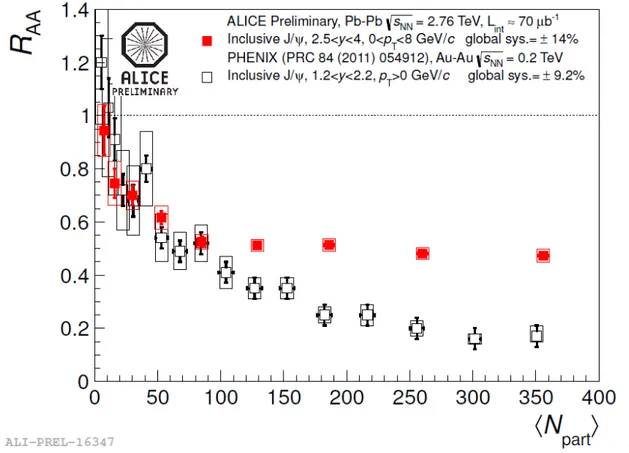
Charmonium states are considered important signatures of the strongly interacting medium created in heavy-ion collisions. In the ALICE experiment, these probes can be investigated

in the µ+µ− decay channel, in the rapidity region 2.5 < y < 4, with transverse momentum

0 < pT < 8 GeV/c. Results on charmonia production in Pb-Pb collisions at

√

s_NN= 2.76 TeV

are presented in figure 1.9. The nuclear modification factor depends on centrality and on the centrality and transverse momentum of the J/ψ particle. It is compared the ALICE experiment result with the PHENIX ones.

The medium dissociation probability of states should provide an estimate of the initial tem-perature reached in the collisions. The studies performed in the last twenty years have shown a reduction of the J/ψ production yield lower than expectations; this is due to the cold nu-clear matter effects. These observations suggest the existence of an additional J/ψ production

mechanism, which sets when higher √sNN are reached. This mechanism can counteract the

quarkonium suppression in the QGP. At high-energy density of the medium and large number

of c ¯c pairs produced in central Pb-Pb collisions, J/ψ production mechanism should help to

Figure 1.9: the J/ψ RAA is shown as a function of nucleons that participate to the collisions

N_part in ALICE experiment and they are compared to the PHENIX result. [9]

1.5.3

Direct Photons

The term direct photons stands for the photons which emerge directly from a particle collision. In heavy-ion collision experiments, the detector captures all the emitted photons including those from the decay of final state hadrons.

More than 90% of the photons in spectrum are emitted from hadron decay. Photons whose are not direct decay product of hadrons represent an important tool for study the evolution of

QGP. Different intervals of pT correspond to photons emitted at different times. It is possible

to subdivide this broad category of direct photons depending on their origin: • prompt photons, which originated from initial hard scattering (hard probes); • pre-equilibrium photons produced before the medium gets thermalized;

• thermal photons originated from quark-gluon plasma as well as from hadronic reactions in the hadronic phase;

• jet conversion photons created from a passage of jets through plasma.

In figure 1.10 are shown direct photons spectra measured in ALICE. It is evident that a greater number of photons are produced at low transverse momenta compared to high

trans-verse momentum. The data are fitted with an exponential function ∝ exp(−pT/Te f f). The

extracted inverse slope parameter is Te f f = 297 MeV in the range 0.9 < pT < 2.1 GeV/c for

the 0 − 20% class, and Te f f = 410 MeV in the range 1.1 < pT < 2.1 GeV/c for the 20 − 40%

centrality class. These values indicate an initial temperature higher than the critical tempera-ture at which the QGP is formed.

Figure 1.10: Direct photon spectra in Pb-Pb collisions at √s_NN = 2.76 TeV for 0 − 20%,

Chapter 2

The ALICE experiment

2.1

The Large Hadron Collider

The Large Hadron Collider (LHC) is located at CERN near Geneva. It is the world’s largest and most powerful particle accelerator, with the first start-up of beams in 2008. Large due to its size, approximately 27 kilometres in circumference, Hadron because LHC accelerates protons or ions at energies up to the record energy 6.5 TeV per proton and Collider because these particles form two beams travelling in opposite directions. The two beams collide at four points, where the two rings of the machine intersect; these are in correspondence of the four particle detector: ALICE, ATLAS, CMS and LHCb, as it is shown in figure 2.1.

CMS ATLAS LHCb ALICE LHC PS SPS PSB AD CTF3 LINAC 2 LINAC 3 AWAKE ISOLDE West Area East Area North Area n-TOF TI2 TT10 TT60 TT2 TI8 protons ions neutrons antiprotons electrons neutrinos

LHC Large Hadron Collider SPS Super Proton Synchrotron PS Proton Synchrotron

AWAKE n-TOF AD

CTF3 Advanced Wakefield Experiment Neutron Time Of Flight Antiproton Decelerator

CLIC Test Facility 3

To avoid colliding with gas molecules inside the accelerator, the beams of particles must travel in the beam pipes in ultralight vacuum. The vacuum is equivalent to pressure to the

order of 10−10 to 10−11 mbar. It is almost as rarefied as the pressure found on the surface of

the Moon. LHC has three separate vacuum systems: one for the beam pipes, one for insulating the cryogenically cooled super-magnets and one for insulating the helium distribution line.

2.1.1

Magnetic lattice

The trillions of accelerated charged particles (protons and heavy-ion) hurtle around the LHC at close the speed of light. They can circle the collider’s tunnel 11.245 times per second. Before they reach the principal ring of LHC, the energy is boosted along the way in a series of interconnected linear and circular accelerators. Once particles reach the maximum speed that one accelerator can lead, they are shot into the next. Beams remain stable on the straight line trajectory due to more than 50 types of electromagnets (dipole magnets), which are needed to send particles along complex paths without them losing their speed.

One of the most complex parts of the LHC are dipole magnets. They generate powerful 8.3 Tesla magnetic field and they use a current of 11.080 amperes to produce field. In addition, a superconducting coil allows the high currents to flow without losing any energy because of electrical resistance. There are 1232 main dipoles, each 15 metres long and 35 heavy tonnes. In addition to just curving the beam, it is also necessary to focus it. Because protons are electrically charged a particle beam diverges if left on its own, due to Coulombian repulsion.

Quadrupoles drive the beams and also keep the particles in a tight beam along the paths.

These have four magnetic poles arranged symmetrically around the beam pipe to force the beam either vertically or horizontally. Schematic configuration of the quadrupoles is shown in figure 2.2.

2.2

The ALICE experiment

ALICE [11] stands for A Large Ion Collider Experiment. The experiment is designed to study the physics of strongly interacting matter at extreme energy densities. This is possible due to the study of heavy-ion Pb-Pb nuclei collisions. In particular, ALICE is optimized for Pb-Pb collisions at a centre of mass energy up to 5.5 TeV per nucleon pair. Therefore, the ALICE Collaboration studies the QGP, the ways it expands and cools down. It tries to recreate labora-tory conditions similar to those just a fraction of the first second after the Big Bang. It tries to show the events before quarks and gluons bind together to form hadron and heavier particles.

The experiment uses the 10.000 tonnes ALICE detector (26 m long, 16 m high and 16 m wide) shown in figure 2.3.

Figure 2.3: ALICE experiment.

2.2.1

The ALICE detector

The ALICE detector is divided into 18 components and each component inspects a specific set of particle properties. These components are stacked in layers, and the particles go through the layers sequentially: outward from the collision point. At first, particles run into the tracking system, then into an electromagnetic (EM) and hadronic calorimeter and finally a muon sys-tem. The detectors are embedded in a magnetic field to bend the tracks of charged particles to measure momentum and charge determination. The aim is to identify all the particles that are coming out from the QGP system.

Figure 2.4: Schematic view of the ALICE detector system. [12]

ALICE uses a set of 18 different detectors that give information about the mass, the velocity and the electrical sign of particles. Schematic representation is shown in figure 2.4. The ALICE detectors can be divided in two main parts, according to the kinematic region that they cover.

At first, there is the central barrel that explore the central rapidity region, and it consists of:

• tracking detectors which are embedded in a magnetic field of 0.5 Tesla; this is produced by a huge magnetic solenoid bending the trajectories of the particles. From the curvature of the tracks, it is possible to derive the momentum of charged particles and their position by reconstructing the vertices of interaction. These are the ITS (Inner Tracking System), the TPC (Time Projection Chamber) and the TRD (Transition Radiation Detector); • Particle IDentification detectors allow to know the identity of each particle, whether it

is an electron, proton, kaon or a pion. This is done using the reconstructing trajectories of tracking detectors. These include the TOF (Time-Of-Flight) and the HMPID (High Momentum Particle IDentification);

• PHOS (Photon Spectrometer) is a high-resolution electromagnetic calorimeter installed in ALICE to provide data to test the thermal and dynamical properties of the initial phase of the collision between ions. In addition, EMCAL (Electro-Magnet Calorimeter) and DCAL (Di-jet Calorimeter) are installed in ALICE for similar purposes.

The second part is dedicated to the complementary rapidity region of the central barrel and it is dedicated to the muon and cosmic rays detection:

• muon spectrometer, formed by MCH (Muon Chamber) and MTR ( Muon Trigger),

stud-ies the complete spectrum of heavy quarkonia via their decay in the µ+µ− channel;

• forward and trigger detectors which are the FMD (Forward Multiplicity Detector), the PMD (Photon Multiplicity Detector), AD (ALICE Diffractive), the ZDC (Zero Degree Calorimeter), V0 and T0;

• cosmic ray trigger detector ACORDE (ALICE Cosmic Rays Detector) detects ray show-ers by triggering the arrival of muons to the top of the ALICE magnet. The ALICE cavern is an ideal place for the detection of high energy atmospheric muons coming from cosmic ray showers.

2.2.2

Inner Tracking System

The Inner Tracking System (ITS) [13] is the innermost tracking detector of the ALICE exper-iment.

Figure 2.5: Schematic view of the six ITS layers and their supporting cones.

Its purpose is to provide both primary and secondary vertices reconstruction and of im-proving the ALICE barrel tracking capabilities closer to the interaction point. Moreover, the

ITS can recover particles which do not reach or are missed by the outermost layers, due to acceptance limitations and momentum cutoff. The ITS consists of six cylindrical layers of silicon detectors. Each layer has a hermetic structure and it is coaxial with the beam pipe. The ITS covers the pseudorapidity range |η| ≤ 0.9 over the entire azimuthal angle, and its radius extends from 3.9 cm to 43 cm. The two innermost layers at 3.9 and 7.6 cm from the beamline are made of Silicon Pixel Detectors (SPD). The two central layers at 15 and 24 cm are made of of Silicon Drift Detectors (SDD); the two outermost ones at 38 and 43 cm are of Silicon Strip Detectors (SSD). In figure 2.5 is shown a schematic view of the ITS layers and its supporting structure.

2.2.3

Time Projection Chamber

The Time Projection Chamber (TPC) [14] is a powerful detector for the three-dimensional tracking of charged particles and identification of ultra-high multiplicity events. The ALICE

TPC has large volume (about 83 m3) filled with gas as detection medium and it is the main

particle tracking device. Only a conservative and redundant tracking device can guarantee reliable performance up to 800 charged particles per unit of rapidity.

The identification of charged particles with low momenta occurs when they cross the gas of the TPC; they ionize the gas atoms along their path, liberating electrons that drift towards the end plates at the end of the detector. The average energy loss by charged particles through collisions with the atomic electrons of the medium is expressed by the relativistic Bethe-Bloch formula dE/dx.

The ALICE TPC has also the task of reconstructing the primary vertices of charged par-ticles beginning from its outermost regions to its core. This is due to different density of charged particles tracks found across the layers: the density is lower in the outermost layers and increases when reaching the innermost ones. The TPC is cylindrical in shape with an ac-tive gas volume that ranges from about 85 cm to 250 cm, in its radial direction, and it has a length of 500 cm along the beam direction as is shown in figure 2.6.

2.2.4

Transition Radiation Detector

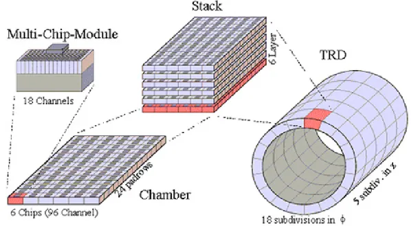
Transition Radiation Detector (TRD) is the main electron and positrons detector in ALICE. It provides this identification using the emission of transition radiation. It is released X-rays when the particles cross many layers of thin materials.

Figure 2.7: Schematic representation of the TRD detector.

The TRD detector [16], shown in figure 2.7, consists of 522 readout chambers arranged in 6 layers surrounding the TPC. They are at a radial distance r (2.9 ≤ r ≤ 3.7 m) from the beam

axis, with a maximum length of 7 m along the beam axis Each chamber is filled with X eCO2

mixture (85:15). The gas volume is subdivided by cathode wire grid into a 3 cm drift region and 0.7 cm amplification region equipped with anode wires.

Figure 2.8: (left) Schematic cross-section of a TRD chamber including radiator. (right) Aver-age pulse height as a function of drift time for pions and electrons with and without transition radiation.

Figure 2.8 (left) shows the cross-section of TRD chamber crossed by a pion and an electron. In addition, in figure 2.7 (right) is also shown the average pulse height, as a function of drift time for pions and electrons with a momentum of 2 GeV/c when passing through the TRD chamber. Comparing the shape of the electrical signal induced by an electron and a pion allows to separate the two particle species by the presence of a long-time peak due to transition radiation photon emitted by the electron in the radiator.

2.2.5

Time of flight

Charged particles in the intermediate momentum range are identified in ALICE by the Time Of Flight (TOF) detector. Time measured with TOF [19] in conjunction with the momentum and with the track length measured by tracking detectors, is used to compute the particle mass. A time resolution of 50 ps will provide 3σ separation up to 2.5 GeV/c for π/K and for K/p separation up to 4 GeV/c.

TOF principal goal is to study:

• The QCD thermodynamics via measurement of π, K and p transverse momentum distri-butions and particle ratios on an event-by-events basis;

Figure 2.9: Schematic view of one of the 18 TOF supermodules positioned along the cylinder. The TOF detector, shown in figure 2.9, is located at a distance of 3.7 m from collision axis. It covers a central region of pseudorapidity −0.9 < η < 0.9 and covers in toto the azimuth. The TOF has a modular structure with 18 sectors in φ , in addition, it has 5 modules along the axial direction. The modules contain a total of 1638 detector elements (MRPC strips), covering an

area of 141 m2with 157.248 channels (pads).

2.2.6

High-Momentum Particle Identification Detector

The High Momentum Particle IDentification (HMPID) is a detector used to identify charged

hadrons with high transverse momentum pT. The HMPID detector has been designed to extend

the useful range for the identification of π/K up to 3 GeV/c and of K/p up to 5 GeV/c. The ALICE HMPID [17], shown in figure 2.10, is formed by Ring Imaging Cherenkov (RICH) counters and consists of seven modules mounted in an independent support cradle. HMPID is fixed to the space frame at a distance of 4.9 m from the centre of collisions, with

a surface of 12 m2. Cherenkov photons are emitted when a fast charged particle crosses the

counter which exploits multi-wire proportional chamber (MWPC) with pad cathode covered with a thin layer of CsI. The Cherenkov photons refract out of the liquid radiator and reach the CsI-coated cathode. MWPC is located at a suitable distance that allows the reduction of the Cherenkov angle resolution because of means of geometrical aberration. The electrons

released by ionizing particles in the proximity gap are filled with CH4 are prevented from

entering the MWPC sensitive volume by a positive polarization of the collection of electrodes close to the radiator.

Figure 2.10: (left) Schematic representation of HMPID detector; (right) schematic representa-tion of MWPC with cathode pads.

2.2.7

Calorimeters

Calorimeters measure the energy of particles and determine whether they have electromagnetic or hadronic interactions. Particle identification in a calorimeter happens when deposition of particle energies occur, except from muons and neutrinos. This is possible because of produc-tion of electromagnetic and hadronic showers when the particles go through the calorimeters.

The electromagnetic calorimeter system of ALICE [18] consists of two detectors:

• PHOS is a high-precision photon spectrometer; its main goal of studying thermal prop-erties of the hot strongly interacting matter created in heavy-ion collisions. To that end,

PHOS measures direct photons radiation at low transverse momenta pT, from hundreds

of MeV to a hundred GeV;

• EMCal is a wide-aperture electromagnetic calorimeter used to explore parton energy loss in the QCD matter. This is achieved by measuring jet quenching as well as prompt

2.2.8

Muon spectrometer

The ALICE muon spectrometer [19] studies the complete spectrum of heavy quarkonia (J/ψ,

ψ0, ϒ, ϒ0, ϒ00) via their decay in the µ+µ− channel.

The spectrometer consists of a passive front absorber to absorb hadrons and photons from the interaction vertex, a high-granularity tracking system of 10 detection planes, a large dipole magnet and 4 planes of trigger chambers. Muons may be identified being the only charged particles able to pass, almost undisturbed, through the absorber.

It provides an essential tool to study the early and hot stages of heavy-ion collisions. In particular, the muon spectrometer is expected to be sensitive to QGP formation. The spectrom-eter covers the pseudorapidity interval 2.5 ≤ η ≤ 4, and the resonances can be detected down

to zero pT. Muons may be identified using the just described technique because they are the

only charged particles able to pass, almost undisturbed, through any material. It happens so because muons with momenta below a few hundred GeV/c do not radiate energy and do not produce electromagnetic showers.

Chapter 3

Reconstruction of non-prompt charmed

baryon Λ

c

with Boosted Decision Trees

technique

3.1

Introduction

The study of charmed-baryon production at the LHC is one of the fundamental tools to verify the theoretical prediction of the state of strongly interacting matter both at high temperatures and densities. These conditions are realised in the early stages of heavy-ion collisions and they create the QGP, as seen in section 1.4.

Due to their high mass, charm quarks are created in the early stages of the collisions in partonic hard scattering. In this environment, the interaction of charm quarks with the medium constituents can modify the hadronisation of quarks: a significant fraction of low and interme-diate momentum charm quarks can hadronise via recombination with other quarks from the medium, while at higher momenta fragmentation processes are dominant. The interplay be-tween these two processes can be investigated with the study of the relative abundance of the different heavy-hadron species produced. In particular, the role of the hadronisation by coa-lescence can manifest in a baryon-to-meson enhancement for charmed hadrons. In this regard,

the study of the Λcplays a key role.

The properties of charmed Lambda baryon*_{Λcare illustrated in table 3.1.}

Symbol Quark content Rest mass (MeV /c2) Mean lifetime (s)

Λ+_c udc 2286.46 ± 0.14 (2.00 ± 0.06) × 10−13

Table 3.1: Main properties of the charmed Lambda baryon.

*_{Lambda baryons are hadrons that contains one up quark, one down quark, and a third quark from a higher}

This heavy particle was reconstructed in ALICE through two hadronic decay channels and a semileptonic one. In this chapter, it is presented the analysis of the hadronic decay

Λ+_c −→ pK_S0. The study is focused on the measurement of the production cross-section of

non-prompt Λc, i.e. Λc coming from beauty-hadrons decays (addressed also as feed-down Λc

in the following, while Λc directly coming from charm quark hadronization are referred as

prompt Λc). Figure 3.1 illustrates the two decay topologies analysed in this chapter. Due to

the short lifetime of the Λc (cτ = 60µm), the low ratio between signal and background and

the limited available statistics collected by the ALICE detector, the reconstruction of Λcdecay

was particularly challenging.

Figure 3.1: Decay of (on the left) feed-down Λcand (on the right) prompt Λc.

Recent results [20] suggested an enhanced production of Λcbaryons at the LHC energies

with respect to theoretical predictions and experimental results from previous experiments at lower energies. Models assuming a large feed-down from higher-mass states has been pro-posed to describe the data. In all the analysis published so far, the correction for the non-prompt

component in the inclusive Λcmeasurements was performed based on theoretical calculations.

Is therefore interesting to investigate the feasibility of data-driven correction approaches for the feed-down correction.

In this chapter it is considered a Machine Learning (ML) technique that uses multivariate analysis (MVA) for classification. For this type of analysis, it is used the TMVA package, distributed within the ROOT analysis framework.

3.2

The Toolkit for Multivariate Data Analysis

The Toolkit for Multivariate Data Analysis (TMVA) [21] is an integrated analysis framework of ROOT [22] that is an object-oriented program and library developed by CERN. The TMVA provides a broad variety of multivariate classification algorithms. All the multivariate tech-niques in TMVA belong to supervised learning. To reach this goal, the algorithms make use of training events, for which the desired output is known. The mapping function can contain var-ious degrees of approximations and it may be a single global function or a set of local models. The machine learning technique chosen is the Boosted Decision Trees.

3.3

Boosted Decision Trees (BDT)

A decision tree, is a binary tree structured classifier composed by a consecutive set of ques-tions: the nodes. A question divides the classification in two samples, called branches. Each question depends on the formerly given answers. The final verdict, called leaf, is reached after a given maximum number of nodes. Figure 3.2 illustrates the schematic view of a decision

tree. The discriminating variable xi is used to bifurcate the data from the root node. The spit

variables used, at each node, provide the best discrimination between signal and background. Thus allowing multiple use of the same variable at several nodes whereas, others are useless. The ending decisions (leaf nodes) label the outputs according to S or B (signal and background respectively); the labelling depends on the events that end up in the different leaf nodes.

Figure 3.2: Schematic view of a decision tree.

A single decision tree is generally unstable because it is prone to statistical fluctuation in the training sample. Besides, a single decision tree can easily be overtrained, i.e. it has a heavy dependence from the characteristics of inputs. To enhance the stability of this method, it is used the boosting algorithm. It is a procedure that combines many weak classifiers to achieve a final powerful classifier. Boosting can be applied to any classification method.

To this end, different trees are produced; their combination, constitutes a random forest. These trees arise from the same training sample and they are built by giving more weight to events that are not correctly identified, as signal or background, by the previous tree. The final output is determined by combined decision of the trees. For the data analysis it has been used the Gradient Boost method, only available for decision trees.

3.3.1

Gradient Boost

Like other boosting methods, gradient boosting combines weak learners into a single strong learner in an iterative fashion. Gradient boosting technique finds the prediction function F(x)

and this is assumed to the weighted sum of parametrised base functions f (x; am). Each base

function in this expansion corresponds to a decision tree:

F(x; P) =

M

∑

m=0

βmf(x; am); P∈ {βm; am}M0. (3.1)

The boosting procedure is now employed to adjust the parameters P such that the devia-tion between the model response F(x) and the true value y obtained from the training sample is minimised. The deviation from this value is measured by the loss-function L(F, y). It is possible to demonstrate that the loss function entirely determines the boosting procedure.

The gradient boost implemented in the TMVA uses the binomial log-likehood loss:

L(F, y) = ln(1 + e−2F(x)y), (3.2)

for classification. As the boosting algorithm corresponding to this loss function cannot be obtained straightforwardly, one has to restore to a steepest descent approach to approach the minimisation. This is done by computing the current gradient loss function and the growing of a regression tree whose leaf values are adjusted to match the mean value of the gradient in each region defined by the tree structure. By iteration of this procedure, it yields the set of decision trees which minimises the loss function.

3.4

BDT Training

The result of running the Boosted Decision Tree algorithm and machine learning in general, can be expressed as a function y(x). This function [23] takes a new digit image x as input and that generates an output vector y, encoded in the same way as the target vectors. The shape of the function y(x) is determined during the training phase, also known as the learning phase, which is based on the training statistical data. Once the model is trained it can then determine the identity of the new digit images, which include a test set. The main task of these types of algorithms is to verify the ability to categorise correctly new events that differ from those used for training, this is known as generalisation. In our case, the algorithm uses the multiclass

methodthat allows to recognise prompt Λc, feed-down Λcand the background signal.

3.4.1

Multiclass

Decision tree learning naturally permit a binary classification. Instead, the multiclass

considered as an extension algorithm of the first binary classifier. Multiclass makes the as-sumption that from each sets of input, it is possible to assign one and only one label (it is not possible, for instance, that one sample can be at the same time prompt and non-prompt).

For the training phase, it is used an adaptation from the TMVA macro tutorials: TMVA-Multiclass.C; while for the application phase it used an adaptation from TMVAMulticlassAp-plication.C.

3.4.2

Monte Carlo simulations

In order to obtain a ML algorithm able to make predictions, it is necessary to build the data sets on which the model training is performed and its performance is evaluated; these are

called training and test sets. The prompt Λc, feed-down Λc and background candidates are

constructed from Monte Carlo (MC) simulation of Pb-Pb collisions measured by the ALICE experiment. The MC consists of a simulation of PYTHIA6 [24] pp events containing charmed hadrons, embedded into an underlying Pb-Pb collision generated with HIJING [25] to obtain a better description of the multiplicity distribution observed in the data; the generated particles were then transported through the ALICE detector by using GEANT3 [26]. The presence of

at least one Λcdecaying via the hadronic decay channel under consideration in each simulated

event was required in order to maximise the number of candidates.

3.5

Input variables

The gradient boost algorithm used for the data analysis used eleven input variables:

1. massK0S: it represents the rest mass of the neutral particle K_S0, reconstructed from the

tracks of its particle daughters after the Λc decay. The particle K_S0 can decay in π+ and

π−. Therefore, from the measurement of their momentum, it is possible to compute the

momentum of the mother particle. It is assumed that for pions the mass is about 138

MeV/c2and the energy of the particle has the form of E_π± =

q

p2

π±+ m 2

π±. Finally, it

is possible to derive the rest mass of K_S0from mK =

q

(E_π++ E_π−)2− p2

K.

2. tImpParBach: proton impact parameter is defined as the minimum distance from the reconstructed track of proton and the position of the primary vertex.

3. tImpParV0: K_S0impact parameter.

4. ctK0S: cτ of K_S0is calculated from the distance of the primary vertex and from the vertex

at which the two pions are created. Then, it is multiplied for the K_S0 mass and divided

by its momentum. This particle has cτ ' 2.68 cm. It is another way to prove that the

5. cosPAK0S: it represents the cosine of the pointing angle, i.e. the angle between the

reconstructed direction of the K_S0 (based on the momenta of the two pions), and the

straight line that links the primary vertex and the decay vertex of the K_S0. It is expected

that the value is close to unity.

6. signd0: the impact parameter of the proton defined with the sign. The sign is defined as positive if the sum of the x-coordinate of the secondary vertex multiplied by the

momentum of the Λc candidate along the x axis and the y coordinate of the secondary

vertex multiplied by the momentum of the Λccandidate along the y axis are greater than

0. The case with signd0>0 is much more compatible with a proton created by the decay

of a Λc compared to the case with signd0<0, in which the proton appears to come from

a point ”before” the primary vertex.

7. DecayLengthK0SXY: it represents the length of the K_S0decay, i.e. the distance between

the decay vertex of K_S0, from which the two pions start, and the primary vertex.

8. NormDecayLengthK0SXY: it is the length of decay of the meson K_S0, i.e. the distance

between the vertex decay and the primary vertex and in the transverse place XY, divided by the error of measure.

9. distanceLcToPrimVtx: it is the distance between the secondary vertex, i.e. decay

ver-tex of the ΛC, and the primary vertex.

10. combinedProtonProb: it quantifies the probability that particle assigned as a proton is effectively a proton. This is possible because of the combination of data recorded by the TOF detector and TPC detector. The TOF uses the difference between the measured flight time from the primary vertex to the detector TOF detector and the expected one in case the particle is a proton, divided by its time resolution. The smaller this difference, the greater the probability that the particle is actually a proton. This difference is usu-ally expressed in units of measurement of the resolution of TOF. The same principle is followed by TPC detector, but in this case, the specific ionization dE/dx for evaluation of different hypothesis it is used.

11. alphaArmLc: it is the longitudinal variable that defines the asymmetry of the decay. If

the pL,p is defined as the parallel momentum of the proton to the momentum of Λc and

p_L,K0

S as the component of meson K

0

S parallel momentum to the momentum Λc, then:

α = p_L,p− p_L,K0 S pL,p+ p_L,K0 S . (3.3)

The training of BDT was repeated independently for two intervals of transverse momentum

and 3.4. In these figures are displayed the superimposition of the two signals (prompt Λc and

feed-down Λc) and the background.

1 − −0.8−0.6−0.4−0.2 0 0.2 0.4 0.60.8 1 d0(bachelor)[cm] 4 − 10 3 − 10 2 − 10 1 − 10 prompt feeddown background 1 − −0.8−0.6−0.4−0.2 0 0.20.4 0.6 0.8 1 )[cm] S 0 d0(K 4 − 10 3 − 10 2 − 10 1 − 10 1 − 10 1 10 102 103 )[cm] S 0 (K τ c 0 5 10 15 20 25 30 35 40 3 − 10 × 0.99 0.992 0.994 0.996 0.998 1 ) S 0 Cosine PA(K 4 − 10 3 − 10 2 − 10 1 − 10 1 2 − 10 10−1 1 signed d0[cm] 3 − 10 2 − 10 1 − 10 0 0.10.2 0.3 0.40.5 0.60.7 0.8 0.9 1 combinedProtonProb 3 − 10 2 − 10 1 − 10 1 1 − 10 1 10 102 3 10 104 DecayLengthK0SXY 3 − 10 2 − 10 1 − 10 1 10 102 3 10 104 NormDecayLengthK0SXY 4 − 10 3 − 10 2 − 10 1 − 10 2 − 10 10−1 1 10 102 103 104 distanceLcToPrimVtx 4 − 10 3 − 10 2 − 10 2 − 10 10−1 1 10 102 103 distanceV0ToPrimVtx 4 − 10 3 − 10 2 − 10 1 − −0.8−0.6−0.4−0.2 0 0.20.4 0.6 0.8 1 alphaArmLc 0 10 20 30 40 50 3 − 10 ×

Figure 3.3: Distribution of input variables for the two signals and background in the pT interval

[2,3] GeV/c. 1 − −0.8−0.6−0.4−0.2 0 0.2 0.4 0.6 0.8 1 d0(bachelor)[cm] 4 − 10 3 − 10 2 − 10 1 − 10 prompt feeddown background 1 − −0.8−0.6−0.4−0.2 0 0.2 0.4 0.6 0.8 1 )[cm] S 0 d0(K 4 − 10 3 − 10 2 − 10 1 − 10 1 − 10 1 10 ₁₀2 3 10 )[cm] S 0 (K τ c 0 5 10 15 20 25 30 35 40 45 3 − 10 × 0.99 0.992 0.994 0.996 0.998 1 ) S 0 Cosine PA(K 4 − 10 3 − 10 2 − 10 1 − 10 1 2 − 10 −1 10 1 signed d0[cm] 2 − 10 1 − 10 0 0.1 0.2 0.3 0.4 0.5 0.6 0.7 0.8 0.9 1 combinedProtonProb 2 − 10 1 − 10 1 1 − 10 1 10 2 10 3 10 4 10 DecayLengthK0SXY 3 − 10 2 − 10 1 − 10 1 10 2 10 3 10 4 10 NormDecayLengthK0SXY 4 − 10 3 − 10 2 − 10 1 − 10 2 − 10 ₁₀−1 _{1 10 10}2 ₁₀3 ₁₀4 distanceLcToPrimVtx 3 − 10 2 − 10 2 − 10 ₁₀−1 _{1 10 10}2 ₁₀3 distanceV0ToPrimVtx 4 − 10 3 − 10 2 − 10 1 − −0.8−0.6−0.4−0.2 0 0.2 0.4 0.6 0.8 1 alphaArmLc 0 5 10 15 20 25 30 35 40 45 3 − 10 ×

Figure 3.4: Distribution of input variables for the two signals and background in the pT interval

It is useful to quantify the correlations between the input variables. The chosen variables are considered a good set if there is a low correlation between them. A correlation between variables exists when there is a relationship that links them. This relationship is quantified by a coefficient that equals 0 if the variables are not correlated. Instead, when the coefficient equals +1 or -1 the variables are totally correlated. The sign of this value states that the two variables are directly proportional (if positive) or indirectly proportional (if negative). The correlation matrices for the two signals and background, labelled respectively:

• signal: it represents feed-down Λc;

• bg0: it represents prompt Λc;

• bg1: it represents the background signal;

in the intervals [2,3] and [3,12] GeV/c are shown in figures 3.5 and 3.6. It is evident that for every matrix there is a high correlation between variables DecayLengthK0SXY and cosPAK0S. 100 − 80 − 60 − 40 − 20 − 0 20 40 60 80 100

massK0StImpParBachtImpParV0cosPAK0Ssignd0 combinedProtonProbCtK0S DecayLengthK0SXYNormDecayLengthK0SXYdistanceLcToPrimVtxalphaArmLc massK0S tImpParBach tImpParV0 cosPAK0S signd0 combinedProtonProb CtK0S DecayLengthK0SXY NormDecayLengthK0SXY distanceLcToPrimVtx alphaArmLc Correlation Matrix (bg0) 100 4 -2 2 -4 1 -7 100 -3 -40 -2 -3 -5 2 -2 2 -3 100 -6 -3 -3 4 -6 100 5 8 -5 6 16 4 -29 -2 -40 5 100 9 3 10 -4 2 -19 2 -2 8 9 100 10 -3 -42 -4 -3 -3 -5 3 100 91 -33 1 -1 -5 -3 6 10 10 91 100 -32 2 -28 1 2 16 -4 -3 -33 -32 100 -2 13 -2 4 2 1 2 -2 100 -4 -7 2 -29 -19 -42 -1 -28 13 -4 100

Linear correlation coefficients in %

100 − 80 − 60 − 40 − 20 − 0 20 40 60 80 100

massK0StImpParBachtImpParV0cosPAK0Ssignd0 combinedProtonProbCtK0S DecayLengthK0SXYNormDecayLengthK0SXYdistanceLcToPrimVtxalphaArmLc massK0S tImpParBach tImpParV0 cosPAK0S signd0 combinedProtonProb CtK0S DecayLengthK0SXY NormDecayLengthK0SXY distanceLcToPrimVtx alphaArmLc Correlation Matrix (bg1) 100 1 1 -5 100 -1 100 1 100 1 -4 -7 9 18 1 -43 -1 1 100 4 1 -4 -4 4 100 -3 1 12 -7 100 87 -23 3 1 9 1 -3 87 100 -24 1 -26 18 1 -23 -24 100 -1 9 1 1 -1 100 -4 -5 -43 -4 12 3 -26 9 -4 100

Linear correlation coefficients in %

100 − 80 − 60 − 40 − 20 − 0 20 40 60 80 100

massK0StImpParBachtImpParV0cosPAK0Ssignd0 combinedProtonProbCtK0S DecayLengthK0SXYNormDecayLengthK0SXYdistanceLcToPrimVtxalphaArmLc massK0S tImpParBach tImpParV0 cosPAK0S signd0 combinedProtonProb CtK0S DecayLengthK0SXY NormDecayLengthK0SXY distanceLcToPrimVtx alphaArmLc

Correlation Matrix (Signal)

100 -1 -5 3 2 2 -5 -1 100 -7 -2 -10 -3 -5 2 2 -5 -7 100 2 1 2 1 -1 -1 -1 3 -2 2 100 -3 11 1 12 7 -3 -31 -10 1 -3 100 7 5 -3 2 -14 11 7 100 11 -4 -2 -45 -3 2 1 100 91 -32 1 2 -5 1 12 5 11 91 100 -31 2 -26 2 -1 7 -3 -4 -32 -31 100 -1 14 2 -1 -3 2 -2 1 2 -1 100 -4 -5 2 -1 -31 -14 -45 -26 14 -4 100

Linear correlation coefficients in %

Figure 3.5: Linear correlation coefficients for prompt Λc, background and feed-down Λc,

100 − 80 − 60 − 40 − 20 − 0 20 40 60 80 100

massK0StImpParBachtImpParV0cosPAK0Ssignd0combinedProtonProbCtK0S DecayLengthK0SXYNormDecayLengthK0SXYdistanceLcToPrimVtxalphaArmLc massK0S tImpParBach tImpParV0 cosPAK0S signd0 combinedProtonProb CtK0S DecayLengthK0SXY NormDecayLengthK0SXY distanceLcToPrimVtx alphaArmLc Correlation Matrix (bg0) 100 -1 6 3 -6 100 9 -1 1 -1 -1 100 4 -2 2 -1 6 4 100 3 -2 9 9 1 -23 9 3 100 3 4 -3 1 -15 -1 3 100 3 -1 -1 -20 1 -2 -2 100 81 -27 2 3 3 9 4 3 81 100 -27 3 -29 9 -3 -1 -27 -27 100 -1 18 2 1 1 -1 2 3 -1 100 -6 -6 -1 -1 -23 -15 -20 3 -29 18 -6 100 Linear correlation coefficients in %

100 − 80 − 60 − 40 − 20 − 0 20 40 60 80 100

massK0StImpParBachtImpParV0cosPAK0Ssignd0combinedProtonProbCtK0SDecayLengthK0SXYNormDecayLengthK0SXYdistanceLcToPrimVtxalphaArmLc massK0S tImpParBach tImpParV0 cosPAK0S signd0 combinedProtonProb CtK0S DecayLengthK0SXY NormDecayLengthK0SXY distanceLcToPrimVtx alphaArmLc Correlation Matrix (bg1) 100 2 2 -6 100 3 100 2 100 2 -5 -7 14 16 1 -41 3 2 100 3 1 -6 -5 3 100 -4 2 15 -7 100 78 -20 5 2 14 1 -4 78 100 -22 1 -33 16 2 -20 -22 100 -1 15 1 1 -1 100 -3 -6 -41 -6 15 5 -33 15 -3 100

Linear correlation coefficients in %

100 − 80 − 60 − 40 − 20 − 0 20 40 60 80 100

massK0StImpParBachtImpParV0cosPAK0Ssignd0combinedProtonProbCtK0S DecayLengthK0SXYNormDecayLengthK0SXYdistanceLcToPrimVtxalphaArmLc massK0S tImpParBach tImpParV0 cosPAK0S signd0 combinedProtonProb CtK0S DecayLengthK0SXY NormDecayLengthK0SXY distanceLcToPrimVtx alphaArmLc

Correlation Matrix (Signal)

100 -1 4 2 -1 1 -6 100 -9 -2 9 -1 1 1 -1 -1 -9 100 -3 4 -2 -3 100 -2 4 4 15 2 -28 2 9 -2 100 1 3 -2 3 -14 -1 4 1 100 -2 -19 -1 1 4 100 80 -27 2 3 1 1 15 3 80 100 -26 3 -29 -2 -2 -27 -26 100 -1 17 -1 2 3 2 3 -1 100 -4 -6 -28 -14 -19 3 -29 17 -4 100 Linear correlation coefficients in %

Figure 3.6: Linear correlation coefficients for prompt Λc, background and feed-down Λc,

3.6

BDT Configuration

The TMVA was configured to use samples for signals and background coming from MC sim-ulations. The good relationship between the performance results of the training and testing

events can assure the success of the training process. The number of prompt Λcand feed-down

Λccandidates are reported: overall in table 3.2, and for each interval of transverse momentum

in table 3.3.

The configuration of the BDT is summarized below in table 3.4.

feed-down Λc prompt Λc Background Total Events

Number of events 34728 34728 2721306 2790762

Table 3.2: Sum of the training and testing events.

Λc pT bin (GeV /c) feed-down Λc prompt Λc Background

2-3 4734 4663 777280

3-12 14800 9851 685414

Table 3.3: Number of training and testing events for the two intervals of transverse momentum.

Option Values Description

NTrees 1000 Number of trees in the forest

MaxDepth 2 Maximum depth of the decision tree allowed

MinNodeSize 2.5% Minimum percentage of training events

required in a leaf node

nCuts 20 Number of points in variable range used

in finding optimal cut in node splitting

BoostType Grad Boosting type for the trees forest

Shrinkage 0.10 Learning rate for GradBoost algorithm

BaggedSampleFraction 0.50 Relative size of bagged event sample

to original size of the data sample Table 3.4: Configuration options used for BDT.

3.7

Training and performance evaluation

The BDT algorithm combines the discriminating power of several input variables to provide a classification tree, which can generate a score when run over data that allows separating