The Productivity Slowdown Puzzle in European Countries

(1)

Dipartimento di Economia, Società e Politica (DESP)

Corso di Dottorato di Ricerca in “Economia, Società e Diritto”

Curriculum Economia e Management

Ciclo XXIX

The Productivity Slowdown Puzzle in

European Countries

Settore Scientifico-Disciplinare: SECS-P/01 Economia Politica

Tutor e Relatore: Giuseppe Travaglini

Co-Relatore: Giorgio Calcagnini

(2)

Abstract

Productivity growth is slowing around the world and this is one of the most disturbing and, no doubt, worrying phenomenon affecting the world economy in the new millennium. The productivity slowdown may appear alarming in relation to the fact that weak productivity growth usually means a lower trend of the whole economy, as well as a lower level of profits, wage and a less public and private debt sustainability.

In this project, our aim is to study the causes of this fall and, in particular, how much and in which manner labour market regulation, and its changes, may affect productivity of labour, capital and the technological progress.

We start our analysis from some stylized facts. Specifically, we use the growth accounting methodology. We collect data for a large group of European and non-European countries and we refer to models related to the economic growth theory. In particular, the exogenous growth theory of Solow (1954) attributes the economic growth to technical progress, and it claim, in its standard formulation, that it does not depend on other economic variables.

In 1963, Nicholas Kaldor listed some stylized facts which seemed to be, with sufficiently widespread, the general empirical regularities of the growth process. Starting from Kaldor model, we will attempt to build an "exogenous" and then an "endogenous" growth model, related to the labour market regulation, which would be coherent especially with the current characteristics of the economic cycle, characterized by a phase of post-crisis and mild economic recovery. Then, with the use of Structural VAR model, we will analyse the responses of three driver variables to three shocks. We will discuss these responses in order to understand the macroeconomic implications. Mainly, the empirical evidence provide support to our view of the complex relationship linking productivity, investment and technological progress with labour regulation in the long run.

(3)

Summary

First Chapter ... 7

Productivity Slowdown ... 7

1.1 Introduction ... 8

1.2 The State of Art: The Productivity Slowdown Puzzle ... 10

1.2.1 The European Framework ... 11

1.2.2 European Monetary Policy ... 12

1.2.3 Euro or not? ... 14

1.2.4 Exchange Rate and Competition ... 15

1.2.5 More in depth: Is the Euro Area an optimal currency area? ... 17

1.3 European Prospective ... 19

1.4 The stylized facts ... 20

1.5 Production, Production Function and GDP: a macroeconomic overview ... 24

1.6 The Unemployment Rate ... 28

1.7 The Inflation Rate ... 31

1.8 The Key Words: Innovation, Investment, Flexibility and Productivity... 32

1.8.1 Positive Correlation ... 34

1.8.2 Negative Correlation ... 35

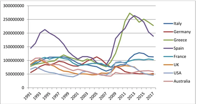
1.9 A Productivity Driver: The Per Capita Income ... 37

1.9.1 Some Data... 38

1.10 External Shock: The Financial Crisis of 2008 ... 45

1.10.1 Consequences ... 47

1.10.2 Impact on Labour Market and Employment ... 49

1.10.3 Measure of prevention ... 51

Second Chapter ... 54

Growth Accounting ... 54

2.1 The Growth Accounting: a brief review ... 55

2.2 The Method... 56

2.3 Some Data... 59

2.4 Technological Progress ... 63

2.4.1 Related Literature ... 66

2.5 Total Factor Productivity (TFP): the key variable ... 68

2.6 Matter of nowadays: Labour Market Flexibility ... 72

2.7 Employment Protection Legislation (EPL) ... 77

2.7.1 Related Literature and Correlation ... 79

Third Chapter ... 81

(4)

3.1 Italian Economic Situation ... 82

3.2 Italian Real Economy ... 84

3.3 Italian Financial Economy ... 90

3.4 A first conclusion ... 92

3.5 Inside Context : Italian Labour Market ... 96

3.6 Italian Prospective ... 98

Fourth Chapter ... 101

Labour Market Models ... 101

4.1 The Labour Market ... 102

4.2 Existing Literature ... 104

4.2.2 Classical Model ... 104

4.2.3 Neoclassical Model ... 108

4.2.4 Keynesian Theory ... 111

4.2.5 The Current Mainstream ... 117

4.2.6 AS – AD Model ... 119

4.2.7 Phillips Curve ... 119

4.3 Growth Models ... 122

4.3.1 Exogenous Growth Models ... 123

4.3.2 The Neoclassical point of view: Solow Model ... 124

4.3.3 A vision to the UK productivity: Pessoa and Van Reenen ... 127

4.3.4 A focus to Unemployment: Layard, Nickell and Jackmann ... 130

4.3.5 Blanchard: The medium Run ... 133

4.3.6 Productivity Differentials in Mature Economies: a Post-Keynesian point of view ... 137

Fifth Chapter ... 142

A Macroeconomic Model of Labour Market ... 142

5.1 Introduction to the Model ... 143

5.2 Assumptions ... 144

5.3 Price Setting ... 144

5.4 Wage Setting ... 147

5.5 The Equilibrium ... 149

5.6 The Long Run ... 151

5.7 A step back: Kaldor Model and Criticism ... 153

5.8 Hypothesis of Shocks ... 158

Sixth Chapter... 164

A VAR Analysis ... 164

6.1 A Micro - Founded Model ... 165

6.2 Long Run Restriction ... 166

6.3 Supply Shocks ... 167

(5)

6.5 Dynamics ... 167

6.6 Estimation ... 169

6.7 The Data and the construction of the Structural VAR Model ... 169

6.8 Stationarity of historical series ... 179

6.8.1 Dicky-Fuller Test ... 181

6.8.2 KPSS Test ... 194

6.9 Analysis of Shocks ... 196

6.10 Time Trend ... 197

6.10.1 Capital shock on capital intensity... 197

6.10.2 Capital shock on the level of technology ... 198

6.10.3 Capital shocks on inflation ... 199

6.10.4 Technological shock on capital intensity ... 200

6.10.5 Technological shock on the level of technology ... 201

6.10.6 Technological shock on inflation ... 202

6.10.7 Demand shocks on capital intensity ... 203

6.10.8 Demand shocks on the level of technology ... 204

6.10.9 Demand shocks on inflation ... 205

6.11 Prime Differences ... 207

6.11.3 Capital shock on inflation ... 209

6.11.7 Demand shock on capital intensity ... 213

6.11.8 Demand shock on the level of technology ... 214

6.11.9 Demand shock on inflation ... 215

6.12 Hodrick- Prescott Filter ... 216

6.12.3 Capital shock on inflation ... 219

6.12.7 Demand shock on capital intensity ... 222

6.12.8 Demand shock on the level of technology ... 223

6.12.9 Demand shock on inflation ... 224

Seventh Chapter ... 227

(6)

7.1 Responses interpretation and macroeconomic implications ... 228

7.2 Concluding Remarks and Extensions ... 231

Appendix ... 236

(7)

First Chapter

(8)

1.1 Introduction

Productivity growth is slowing around the world, and this is one of the most disturbing and, no doubt, worrying phenomenon, that is affecting the world economy in these first years of the new millennium. The productivity slowdown may appear very alarming in relation to the fact that, as it is well known, its weak growth usually means a lower trend growth of the economy, as well as a lower level of firms’ profits, a lack of wage trends and less debt sustainability.

In this project, our aim is to understand how much and in which way labour flexibility, introduced since the early 90’s in Italy and in the most Western European countries has affected the productivity of capital, the productivity of labour and the technological progress. Our intent is also to try to find and to understand the causes of this fall. The evidence shows that in the last fifteen years, so since the early Nineties, most of the European countries, and especially among them Italy, are going through a period of clear economic decline. Theyhave recorded the worst economic performance from the end of the Second World War accompanied, paradoxically, by increased employment, until the last few years. The symptom more evident of this stagnation has been the slowdown in the growth rate of labour productivity. Until the late eighties, instead, although in a context of a general reduction in the growth, the productivity of European countries remained higher than the US. It is therefore necessary to understand the roots of this negative situation, investigating the functioning of the labour market and the model adopted by these countries, in particular the role played by flexibility, in order to understand which variables are more or less involved.

The project is divided into seven chapters and it is organized as follows. In the first one, we will present the problem of the productivity slowdown, trying to find out the possible causes and to understand the variables involved in this kind of phenomenon. We will start describing the economic situation of Europe, to make an idea of which is the general economic trend of the countries, with a detailed description of the variables involved, in order to have a clearer picture about the trends of innovation, technological progress, investment, capital accumulation and productivity, which are the drivers of the economic growth.

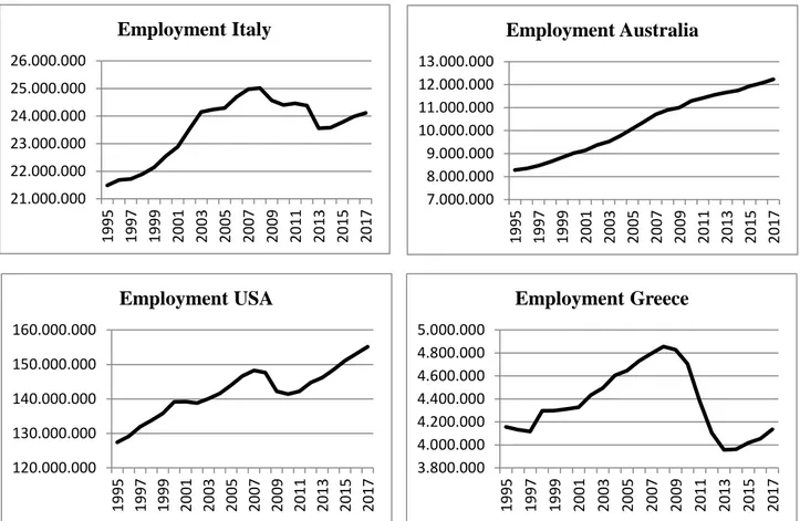
In the second chapter, we will describe the theory of Growth Accounting, in order to reach the definition of Total Factor Productivity (TFP), a key element of the analysis. To make a clear and complete analysis, however, it is fundamental collecting specific data. We will use the Ameco database of the European Commission for both European countries and for USA and Australia, so that it will be possible to make comparisons among them.

Our intent is to go more in deep, analysing which is the economic situation of a specific country, so the third chapter focus on the Italian case. Italy, indeed, has gone and it is still going through a moment of decisive changes, due to several structural reforms and to different European economic policy measures. Despite being among the most industrialized countries and between the world powers, it has shown in the last twenty years strong weaknesses both in the real economy and in the financial economy.

The fourth chapter makes an overview of all the most important labour market models, that over the years have been developed by the leading economists and by the

(9)

main schools of thought, until arrive to the most recent dynamic growth models. It is from these last models, in particular focusing on Solow and Kaldor model, that we lie the foundations for the construction of a new model with similar characteristics but more near the current economic situation and business cycle.

Our goal in the fifth chapter is to build a theoretical exogenous growth model, which can involve all the key variables necessary to describe the condition of the labour market. We construct a Price – setting and Wage - setting model and we test what happen to the system if we introduced shocks.

We will make, moreover, in the sixth chapter, an empirical verification with the construction of a micro-founded model. We will estimate, with the use of Structural VAR, the responses given by three driver variables (capital intensity, Total Factor Productivity and GDP Price Deflator) to three shocks (two supply shocks, capital and technological shocks, and a demand shock). These responses permit us to understand the macroeconomic implications for the system that lies behind supply and demand shocks.

In the seventh chapter, we summarize the work done along the project, the variables involved, in order to analyze the productivity slowdown phenomenon, the literature contribution studied to construct our model, the results obtained. Our aim is to have a desirable confirmation of the initial hypotheses presented, and, hopefully, the possibility to make forecasts and prevention for the future.

(10)

1.2 The State of Art: The Productivity Slowdown Puzzle

Let us start seeing more in depth, which is nowadays and which has been in the last years the situation of the economies on the world and especially the European countries’ economies, in order to focus on our main problem. With the end of the twentieth century and the beginning of the new millennium in European countries and especially in developing countries, like Italy, experience a structural change in the trend of economic growth. This change is reflected in an increasingly marked slowdown in the GDP growth rate and in the deterioration of labour productivity, real investment and international competitiveness. Interpreting this Long-Term phenomenon is not easy. Between the late eighties and the first years of the new Millennium, the organization of European labour markets changes profoundly towards increasingly deregulated, flexible and precarious forms and contracts. Parallel it is revolutionizing the organization of international financial markets, expanding with ever experienced before capital mobility modes. New emerging countries such as China and India entering the global stage, they change, but in a direction still to be defined, the balance in Middle East, with the inevitable tensions in the markets of oil products and the Mediterranean geopolitics.

In short, the process of globalization and liberalization of markets pushes the world economy, and especially the European economies, along a ridge unprecedented growth path of new unknowns and with a predominantly liberal character, both economic and social, that had sustained European economic development from the post-World War II onwards. In seeking to understand this problem, it is tempting to invoke the global financial crisis that erupted in 2008. It disrupted the availability of credit, which is important for innovation, and it slowed the growth of international trade, with which increases in productivity and technical efficiency are associated historically. There seems to be substantial agreement among scholars that the productivity slowdown level is only partly attributable to the crisis of 2008 and that it refers to deeper economic problems.

Among other things, the phenomenon began to manifest itself in the early years of the new millennium, although it has since worsened. The crisis has reduced, however, the flow of credit for firms’ investment by the banking system, which had to keep locked resources in firms in difficulty, not so able to direct funding towards new sectors with higher productivity. Firms are parallel become more cautious, preferring to maintain high liquidity rather than embarking on risky projects. On the other hand, the crisis has helped keep wages low, thus reducing the incentives of firms to substitute capital for labour. Meanwhile, in the public sector austerity policies and other difficulties they have led to the reduction in the various countries also increased government investment.

A common explanation of the productivity slowdown phenomenon refers to some changes in the structure of economies. Therefore, the argument is that rich countries, which have already recorded a strong level of automation in industry, are developing their activities in the service sector, which has fewer spaces for rapid gains in efficiency and that has not been invested in massively from automation processes.

Simon Taylor (2016) has recently advanced a new hypothesis. In the last period, says the author, the degree of concentration of many sectors is increasing significantly, from telecommunications, social media, to internet search engines, pharmaceuticals, electronic commerce, etc. On the other hand, he notes that the anti-trust authorities have

(11)

slowed their pressure on firms. The scholar concludes that this trend can be explained at least in part the productivity slowdown, because in a monopolistic situation, the undertakings, having less need to generate adequate profits, have incentives to invest less in innovation.

Another important explanation relates to the field of high technologies refers to the finding that the innovations are no longer passing quickly from the few progressive firms in the rest of the economy, as happened once; the diffusive machine is jammed (O'Connor, 2016), perhaps, again, to increase the monopoly power of a few large firms.

Another possible evaluation would have to do with the quality of work. While employees with high qualifications are retiring, a workforce that is less competent and efficient, because studied less gradually replaces them. Of course, the segment of the population that is less educated today is that of the poorest and weakest.

A more technical consideration, finally, has to do with institutional factors, such as education and vocational training quality, the public infrastructure, the organizations that promote entrepreneurship, etc. All these activities in the last times are suffering a lot due to lack of resources.

Nevertheless, the slump in the Total Factor Productivity, which is the driver for the growth, as we will demonstrate ahead in the research, is widespread. It is not limited to or even differentially evident in countries most directly affected by the financial crisis. In the advanced countries, where the deceleration in productivity growth predates the financial crisis, some observers have invoked the hypothesis of secular stagnation, suggesting that productivity growth has slowed because of a decline in innovation or, possibly, inadequate spending on the demand side. For this reason, there will be the technical progress and the trend of the aggregate demand the variables involved in our studies, in order to get some results that could explain the problem of productivity slowdown. We will describe in the next paragraphs the general economic situation of European Countries, to go then more in depth to the causes of our problem.

1.2.1 The European Framework

The economic crisis, the demographic challenge, migration, youth unemployment and the Transatlantic Treaty: a synthetic analysis of the field of problems across the Union in the recent years. What is most alarming, however, is that in the last fifteen years, European countries have recorded the worst economic performance since the end of the Second World War. This disappointing evolution has been the subject of increasing scrutiny over recent years.

We can distinguish, at a glance, two revolutionary facts, which have struck Europe in recent years: one from a “real” point of view, the deregulation of the labour market, resulting in a greater flexibility within the same and the other one that interest the “monetary” sphere, the introduction of the Euro, the single currency. These two phenomena, combined together, have generated significant consequences, both on the side of the real economy and on the side of the financial economy, which are synthesized in the fall in productivity of both labour and capital and in serious consequences on employment and investments.

(12)

Starting from the real side, since the launch of the Lisbon agenda in 2000, about ten million labours have been created in the EU. This strategy has provided a satisfactory answer to the problem of the rising European unemployment of the 1980s, but many countries have seen labour productivity decline over the same period. Thus, after the labourless growth of the 1980s and early 1990s. One first possible explanation to this phenomenon is that the rise in employment itself has caused the productivity slowdown. A short-run trade-off between employment and productivity may indeed emerge if the rising employment entails a lower capital per worker, and if more workers with relatively low skills are employed. Most of the recent literature has focused to shocks to labour supply, such as changes in real-wage aspirations and labour market institutions, to explain differences in economic performance among countries. In this perspective, the productivity slowdown in the EU15 is only a short run effect of the increase in the employment rate, with productivity recovery in the long run. However, in principle, any number of causes can explain the current trade-off between employment and productivity, including a deceleration of the technological progress, a decrease in the ratio of capital stock per worker, an adverse effect of the composition of labour supply due to recent immigration, changes in labour market policies and institutions, variations in the distribution of income with unfavourable consequences on profits and investments, or any combination of these. We address the question of whether the shift in the labour supply curve is the only fundamental change capturing the negative correlation between the growth rates of productivity and employment. If this explanation is correct then the labour demand curve did not shift in recent times, keeping other features of the production function unchanged. This problem of identification may account for the mixed empirical results found by several authors on the relationship between productivity and employment.

1.2.2 European Monetary Policy

As we have already said before, from a monetary aspect, the introduction of the single currency has determine some consequences in the real economies of the countries involved. Let us analyse the situation.

As it is known, the European Union has experienced a very important and fundamental event. In 1999, indeed, the European Union decided to go one-step further and started the process of replacing national currencies with one common currency, called the Euro. Only eleven countries participated at the beginning; since then, six more have joined. Some countries, in particular the United Kingdom, have decided not to join, at least for the time being. The official name for the group of member countries is the Euro Area. The transition took place in steps. On the first January, 1999, each of the eleven countries fixed the value of its currency to the Euro. For example, a Euro was set equal to 6.56 French francs, to 166 Spanish pesetas, and so on. From 1999 to 2002, prices were quoted both in national currency units and in Euro, but the Euro was not yet used as currency. This happened in 2002, when the Euro notes and coins replaced national currencies. Seventeen countries now belong to this common currency area. So nowadays, the European Central Bank (ECB) and the European System of Central Banks (ESCB),

(13)

which are independent from other EU institutions and from national governments, manage the monetary policy. The primary objective of the European monetary policy is the price stability, defined as "a situation in which the 12-month increase in the consumer prices for the euro area is less than the 2% over the medium term time horizon”. Therefore, the first target of the EBC is the inflation.

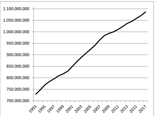
Figure 1. Euro Area Price Deflator Gross Domestic Product

Sources: AMECO - Annual macro-economic database – European Commission

Figure 1 shows the trend of the Price Deflator of Gross Domestic Product for the Euro Area from 1993 until 2017. This variable is a driver for the inflation. It is easy to see that the line is stably increasing, reflecting the limit of 2% imposed by the monetary authority. This goal, the monetary stability, is essentialin order to ensure the maintenance of price stability in the euro area and to preserve the international value of the euro, i.e. its purchasing power.

However, there are other secondary objectives as much important, such as the economic development, the employment, the social and the environment protection. The ECB's strategy, therefore, is based on two pillars: the control of the money and the maintenance of stable inflation in the medium term. The instruments used are the official rates, the reserve requirements for financial intermediaries, the open market operations, direct controls (supervision); through channels such as the interest rate, the exchange rate, financial asset prices, bank lending channel, financial credit channel. A restrictive monetary policy implies a reduction in aggregate and an increase in the monetary interest rate (on deposits), conversely an expansionary policy entails an increase of the currency and a reduction in the rate. With the creation of the European Monetary Union, through the Maastricht Agreement of 1992, in any case, the changes were not only institutional with the transfer of responsibility for monetary policy from national central banks to the

700.000.000 750.000.000 800.000.000 850.000.000 900.000.000 950.000.000 1.000.000.000 1.050.000.000 1.100.000.000

(14)

ECB, but also economic and share with the entry into circulation since 2002 of the single European currency, the Euro. This event, in fact, has brought with it a series of above all financial consequences, but undoubtedly linked to the real economy, which generated in the majority of acceding countries to the union, a lot of internal imbalances that need a reorganization through economic policies adequate. Anyway, a monetary union not accompanied by a fiscal and political union, as we will see in the following paragraphs from the data that describe the recent European situation, hardly can stand.

1.2.3 Euro or not?

Since its entry into force, the single currency was seen as a new problem for the European Union. Economists and citizens are divided between those who are in favour of its circulation and those who are against it.

Supporters of the euro point out first to its enormous symbolic importance. In light of the many past wars among European countries, what better proof of the permanent end to military conflict than the adoption of a common currency? They also point out to the economic advantages of having a common currency: no more changes in the relative price of currencies for European firms to worry about, no more need to change currencies when crossing borders. Together with the removal of other obstacles to trade among European countries, the euro contributes, they argue, to the creation of a large economic power in the world.

Others worry that the symbolism of the euro may come with substantial economic costs. They point out that a common currency means a common monetary policy, which means the same interest rate across the euro countries. What if one country plunges into recession, while another is in the middle of an economic boom? The first country needs lower interest rates to increase spending and output; the second country needs higher interest rates to slow down its economy. If interest rates have to be the same in both countries, what will happen? Is not there the risk that one country will remain in recession for a long time or that the other will not be able to slow down its booming economy?

Until the first years of the adoption of Euro, the debate was somewhat abstract. It no longer is. A number of euro members, from Ireland, to Portugal, to Greece, are going through deep recessions. If they had their own currency, they likely would have decreased their interest rate or depreciated their currency so that they would see to increase the demand for their exports. Because they share a currency with their neighbours, this is not possible. Thus, some economists argue that they should drop out of the euro. Others argue that such an exit would be both unwise, as it would give up on the other advantages of being in the euro, and extremely disruptive, leading to even deeper problems for the country that has existed. This issue is likely to remain a hot one for some time to come. (Blanchard, 2012).

(15)

1.2.4 Exchange Rate and Competition

In 2013, the Italian President of the ECB, Mario Draghi, said that the euro exchange rate has very much appreciated against all the major currencies, indicating a return of the confidence in Europe. No doubt, it was an affirmation to encourage the exit from the crisis and from the economic pessimism climate that was present in the operators early as the 2008 outbreak. Nevertheless, a strong national currency against foreign ones, is really a good thing and to be happy about? If we look at foreign and international context, the productivity of a state must necessarily be related to the competitiveness and the economy of that country is able to support than the others. This aspect is more significant for Italy, if we consider that it as well as one of the world state is inserted in the complicated and ever-changing European context. Intuitively, the notion of competitiveness can be immediately linked to the relative comparison between the growth rates of different countries but also to the evolution of a commercial nature, and international agreements with the related benefits that may ensue.

We can distinguish two main meanings of competitiveness, a short-term price competitiveness, linked to changes in the real exchange rate and the consequent change in unit production costs; and a long-term competitiveness of technological character. Whereas the nominal exchange rate is defined as the price of foreign currency in terms of national currency, while the real exchange rate is the ratio between the prices of domestically produced good, expressed in local currency, and the price of foreign production good, which is also expressed in local currency. Therefore, we can consider the following relationship:

𝑅 = 𝑃1/𝐸𝑃2 (1)

where:

𝑃₁ : price of domestically produced expressed in domestic currency (e.g. €) 𝑃₂ : price of foreign production expressed in foreign currency (e.g. $) 𝑅 : the real exchange rate

𝐸 : the nominal exchange rate (e.g. € / $)

If 𝑅 is increasing, it has an appreciation and it determines a decrease in the price of international competitiveness for the local producer, while if 𝑅 is descending, it has a depreciation with a consequent increase in the price of international competitiveness for the local producer. Price competitiveness can be obtained with a devaluation of the nominal exchange rate, i.e. an increase of E, or by a decrease in the price of locally produced goods (𝑃1) obtained by reduction of unit costs. The depreciation of the real

exchange rate can be achieved with a reduction of the debt, as lower debt implies lower interest rate, possibility of more investment abroad, decrease in national currency value. This, however, is not a sustainable strategy in the long run, in fact if the price of imported goods increases, the inflation increases, causing a fall in domestic investment and consequently in productivity. The long-term technological competitiveness is determined by innovation, which implies higher productivity and exports, it is compatible with products of the highest prices (higher quality indicators) and a higher value of the national

(16)

currency. It implies the idea that relations between countries can be characterized as a positive sum game rather than a game to zero sum. How to increase the long-term competitiveness is the main question that arises the theory of growth.

The introduction of the single currency in Europe, determined, with no doubt, major changes in the international monetary environment. They were born new relations of exchange rate between the Euro and other major currencies like the US dollar, the British pound and the Japanese yen. The euro-dollar relationship, especially, it is significant to have a comparison between the performance of the European economy and the American economy. The historian of the euro-dollar exchange rate was established, as opposed to many those who think, already in 1999, and not in 2002, the official year when the euro was introduced into people's pockets. For accounting purposes, and within the financial markets, the euro was born in the past millennium, namely the first January 1999, when it began to be traded within such financial transactions. It is on that date that is born historian of the euro-dollar exchange rate, along with historical graphs of exchange rates between the euro and other currencies. From the birth of the historian of the euro-dollar exchange rate it has been 3 years before the euro began to circulate in the pockets of the Europeans, or rather, in the countries of Europe who have agreed to use the euro as their single currency.

Therefore, if the 1999 was the date when our currency has started to be used for financial and accounting transactions, the euro-dollar exchange rate (EUR USD) came in 2016 in his eighteenth year of age. It is considered nowadays the most famous exchange rate in the world, the most absolute liquid and the most chosen by investors, because it allows earning money by investing both in the long and in the short-term. How was the euro-dollar exchange rate trend during these years? What were the peaks and the minimum of this relationship? In what way can we use the historical data to invest in the future and to make forecasts? Let us see more in depth, which has been the trend of the euro-dollar exchange rate over the years in the graph below, in order to answer our questions.

(17)

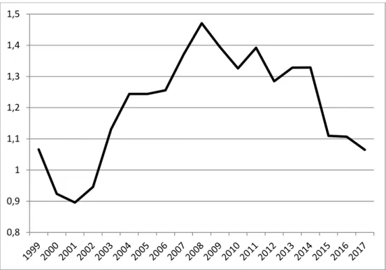
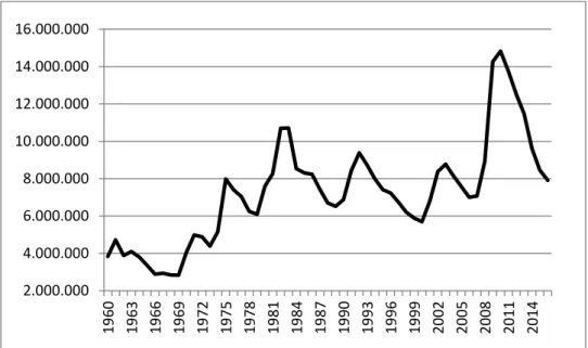
Figure 2. Annual EUR USD Exchange Rate. Source: FRED- Federal Reserve Economic Data

From an historical graph of euro-dollar exchange rate, in Figure 2, we can note what the initial effects on the economy were.At birth, in 1999, the euro-dollar was quoted at 1.18, meaning that for 1 euro corresponded as much as 1.18 US dollars. The euro dollar moved a lot over the years and it is precisely for this reason that it has earned the nickname of “couple of more volatile currencies in the world”. Something that could has been expected if we consider that the US is the first economy in the world and Europe is just behind. The minimum value of all time was 0.83, reached in 2001, while the maximum was 1.60 US dollars, reached in October 2008, with explosion of the financial crisis. Between one and the other of these intervals of time, we have seen a trend variable and very volatile, often linked to the logic of supply and demand. Macro-economic issues and fundamental analysis, such as Quantitative Easing by the Fed before and by the ECB then, or the movements of interest rates, but also the trend of unemployment, influence it. After 2008, the trend continue to be quite variable and a bit decreasing. Between 2015 and 2016, cause of the outbreak of the crisis in Greece and the launch of Quantitative Easing by Mario Draghi, the euro-dollar exchange rate comes to a level around the value of one. So much that many investors thought that it would find the equality (one euro for one US dollar) in 2016, but this has not happened yet.

1.2.5 More in depth: Is the Euro Area an optimal currency

area?

The theory of Optimum Currency Areas (OCA) investigates the costs and the benefits that might arise for countries that choose to join a monetary union. It builds its

0,8 0,9 1 1,1 1,2 1,3 1,4 1,5

(18)

foundations on the school of thought called neoclassical synthesis, according to which the level of aggregate demand in the long run, will match the level of production by the change in relative prices of goods and inputs. Aggregate demand determines the level of production only in the short term, thereby taking up the Keynesian idea of the centrality of the question.

The main criterion that should satisfy optimum currency area lies in the full capabilities of money wages and prices from falling down. Because of asymmetric shocks hitting one of the region which result in a drop in production and employment in the affected region, flexible money wages down would lead to a decrease in prices, an increase in the affected region and therefore exports to increased production and employment, thanks to a change in consumer preferences. Another way by which the reduction of money wages leads to an increase in output and employment it is the most complicated Keynes effect, focused on domestic demand.

The theory of optimum currency areas argues that the single currency favours the mobility of factors of production (capital and labour) and greater financial integration between countries outside the currency. The mobility of the work allows, in the idea of Mundell, to be able to deal with an asymmetric shock by a region that undergoes the shock. The mobility of capital, virtually the same thing in financial integration, allows the convergence of interest rates in the countries belonging to the area (we showed in an article here as in the euro convergence in interest rates on bonds public has been allowed thanks to the ECB's monetary policy) due to the absence of exchange rate risk.

The main problem that is taken into consideration when it comes to understanding the advantages inherent in creating an area of fixed exchange rates or a monetary union is the possible occurrence of asymmetric shocks in the exogenous variables of the countries involved. An example is given by an asymmetrical variation (which occurs in one or more countries, but not in all) produced in a country (country A) may increase, while it might decrease the demand for goods produced in another country (country B). In the absence of a system of fixed exchange rates, the increased demand for goods in the country should to change the exchange rate. This leads to the depreciation of the currency of country B and the appreciation of the currency of country A. The increase in unemployment (or the deterioration of the trade balance) is avoided in country B. Clearly, this adjustment cannot take place in the presence of fixed exchange rates, or even of a monetary union regime. The adjustment could be achieved by a change in wage and price, should they be flexible. In the absence of this flexibility, the only solution to avoid the consequences of the shock would be the shift of production factors.

As regards price changes, then hire them, as possible (flexibility of prices and wages) is not enough to consider them a remedy. In fact, it would be necessary that the economies of the two countries were closely integrated from the commercial point of view: in this way, a small decline in prices of goods produced in country B would lead to a sharp increase of their demand. Another element that may facilitate optimum currency area is the actual presence of a fiscal federalism system, useful in mobilizing resources from the most advantaged areas to the most disadvantaged. A result of these considerations is that currency (or monetary) area is optimal if asymmetric shocks are rare or absent, or if prices and wages in the various countries are very flexible, or if the

(19)

economies of the two countries are highly integrated. Alternatively, an efficient fiscal federalism system could make more desirable monetary integration.

Theorists of OCA point out that because a currency area can be defined as optimal, it is necessary the existence of a both monetary and fiscal union. This means the existence of a common public budget to the entire area, so that any asymmetric shocks can be addressed with appropriate automatic stabilizers, i.e. fiscal transfers in favour of the regions that show a loss of production and employment. This is a delicate point of the question, as the Eurozone, unlike what happens in the US, is not a fiscal union. With the Euro, monetary policy has become common, but the fiscal policy decisions are taken individually by each country (though bound by the Maastricht Treaty). It lacks a centralized transfer system, able to support the spending capacity of the countries in difficulty. We can then also respond, as they have done, however, in many, that the Eurozone is not an optimal currency area. The bottom line, however, remains one regarding a review of a policy that, at the base, is very little founded.

1.3 European Prospective

The recovery seen in recent quarters in Europe is still modest and fragile. The weakening external demand and uncertainties in the global outlook have increased the risks of a global economic slowdown. An extended period exceptionally low inflation and slow recovery are affecting negatively the growth potential and weakening expectations about future economic prospects. Critical indicators such as investment, industrial output and employment are still far below pre-crisis levels in several Member States. Imbalances have expanded further, with negative consequences on the overall sustainability and the resilience of the euro area.

The signs of disaffection with the European project are much more widespread than we could fear at the height of the crisis, whose exceptional durability powered consent for populist proposals. These are favored also by the difficulty to perceive the added value of EU membership. On the contrary, especially in some countries the response to the crisis was regarded as likely to exacerbate divisions between the center and periphery of the Union. Overall, the mix of policies implemented in the Euro zone has proved inadequate to address the crisis and stimulate a sustained recovery. To prevent that significant and persistent loss of the product influence in a permanent way the potential growth, further convergence, acceleration of structural reforms and strong domestic demand are necessary. Beyond the current policy mix and the positive contribution made by the orientation of the ECB, serve coordinated and decisive actions to address urgently the challenges of restoring growth sustained and positive expectations. Europe is also facing new exceptional systemic challenges: the influx of migrants and asylum seekers. These challenges require a coordinated policy for provide immediate help and to plan joint initiatives that facilitate the integration. Any tightening of controls at internal borders to the Union would be detrimental to the free movement of workers and goods, with negative consequences from the impact unpredictable. Adequate policies in this field can only be adopted following a integrated approach, in which the implementation of short term initiatives is part a more ambitious strategy.

(20)

Although in most countries production has picked up again, in many member states of Eastern Europe and South it remains below the level of 2007. We need a strong macroeconomic stimulus, boosting growth and employment. Monetary policy has been strengthened in the expansive way through quantitative easing. However, in the current macroeconomic context marked by low expectations and weak demand, this will not encourage them to return. The so-called Juncker Plan, for the same reasons, will not provide the necessary stimulus to the economy, while the new interpretation of the Stability and Growth Pact, which leads despite some progress, will result only in reducing the tax burden in countries in crisis, instead of generating a substantial fiscal stimulus. It requires coordinated economic expansion, focused on boosting employment through the realization of investments that promote the environment, conscious gender optics; the attack on social spending has to stop. The single currency should be supplemented with an active fiscal policy at the federal level, which is able to operate effectively in stabilizing countercyclical key regional, national and federal and, at the same time, to operate the transfer of resources between the richest regions and the poorest. Fiscal policy should be highly progressive and integrated by European unemployment insurance, acting as a key automatic stabilizer. Of the structural and regional policies of the EU should be strengthened and extended, especially through a large program of public and private investment, financed by the European Investment Bank, and focuses in particular on countries in deficit, and on those with low income.

1.4 The stylized facts

Summing up all the considerations made in the previous paragraphs, we can outline four conflicting stylized facts, which characterizes the economic decline in Europe and especially in Italy in the last two decades:

1. The increase in employment. Much of the literature about the issue of the recent Italian and European stagnation has placed at the core of the functioning of the labour market, with an emphasis on the mechanisms that regulate the labour supply. The models based on labour explain the productivity slowdown in European countries because of the downward shift of the supply curve: the low productivity growth is just a short-term effect due to growing employment, with productivity that will recover in the long run due to higher activity levels. The increase in employment rate is due to important reforms and changes in labour market, connected to a strong wage flexibility especially over the course of the 1990s.

(21)

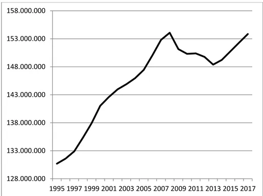
Figure 3. Employment, persons: total economy, Euro Area

Figure 3 shows the trend of the employment in the Euro Area from 1995 until now. From the first years until 2009 the values increase considerably, starting from a value of 130.000.000 persons employed to almost 155.000.000 persons. From 2009, in the peak of the financial crises, the trend start to decreases slightly and the number of persons employed was less than 150.000.000 in 2013. In the last few years, however, the values seem to rise again reaching more or less the same value of 2009.

2. The productivity slowdown. There is a negative correlation between the growth rates of employment and the growth rate of productivity; in particular, there is a slower growth of output per worker, connected to a slower capital stock per worker. There is also a change in the composition of labour supply due to recent immigration, with negative effects on productivity.

128.000.000 133.000.000 138.000.000 143.000.000 148.000.000 153.000.000 158.000.000 1995 1997 1999 2001 2003 2005 2007 2009 2011 2013 2015 2017

(22)

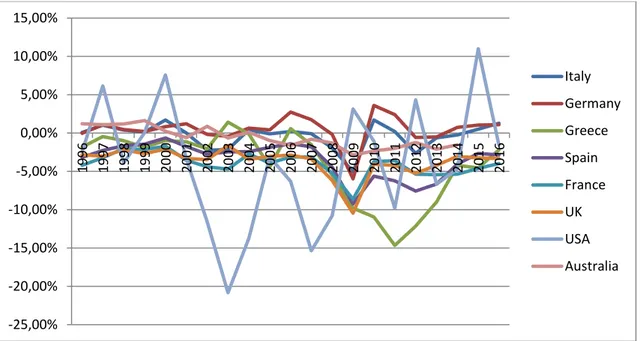
Figure 4. Annual logarithmic differences of Euro Area TFP

Figure 4 shows the trend of the annual logarithmic differences of TFP in the Euro Area from 1995 until 2016. The curve is not linear there are a lot of peaks and minimum. In particular it evident to see the minimum peak in 2008, with a negative difference of 5% from the previous year. In 2009, the difference is recovered, but in 2011, it falls again of about 3%. In the last few years, the trend seems to be more stable and slightly increasing.

3. The rise of profits. There has been a shift in income distribution with different consequences on profits and accumulation.

4. The fall of capital intensity. The growth rate of the capital deepening (the rate of investment per worker) has decreased, signalling that firms invested in capital saving production and they prefer low quality work, generating a low level of technological progress. -4,50% -3,50% -2,50% -1,50% -0,50% 0,50% 1,50% 2,50% 19 95 19 96 19 97 19 98 19 99 20 00 20 01 20 02 20 03 20 04 20 05 20 06 20 07 20 08 20 09 20 10 20 11 20 12 20 13 20 14 20 15 20 16

(23)

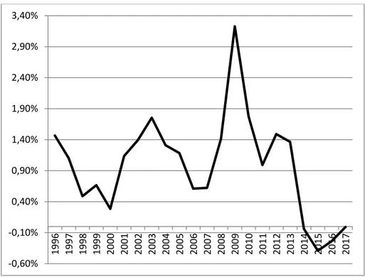
Figure 5. Annual logarithmic differences of Euro Area Capital Intensity Sources: AMECO - Annual macro-economic database – European Commission

Figure 5 shows the trend of the annual logarithmic differences of Capital Intensity in the Euro Area from 1995 until 2017. The curve is not linear. It is evident the increase from 2007 to 2009 for about 3% and the consequent slowdown until 2011 with a negative different of more than 2%. Until 2013, the gap seem to recover but there is a reduction of about 2%. In the last few years, the trend seems to increase slightly.

These changes in the capital-labour ratio may reflect that the adoption of technologies is not neutral, with consequences on growth and income distribution. Moreover, we can distinguish two types of shocks that hit the Europe and the Italian economy in the last fifteen years, causing the so-called “Productivity Slowdown Puzzle”:

1. Non-Technological (or Institutional) Shocks 2. Technological Shocks

These shocks have shown their effects in the labour market affecting employment, productivity, wages, profits and growth. The Non Technological Shock are all shocks that increase the supply of labour (moving the supply curve of labour) such as the introduction of reforms in the labour market. We can consider, among them, also the wage moderation, the reorganization of the legislation in the labour market (in Italy the reforms of Treu and Biagi), the double-level wage bargaining, the immigration of low quality labour (human capital): they have all changed the characteristics of the labour market and employment. Adverse Technological Shocks, instead, are all shocks that affect the labour demand (shift of the labour demand curve). Therefore, we have the reduction of the Total Factor

-0,60% -0,10% 0,40% 0,90% 1,40% 1,90% 2,40% 2,90% 3,40% 19 96 19 97 19 98 19 99 20 00 20 01 20 02 20 03 20 04 20 05 20 06 20 07 20 08 20 09 20 10 20 11 20 12 20 13 20 14 20 15 20 16 20 17

(24)

Productivity growth (which we will analyse in the next paragraphs), with consequences on the productivity slowdown, in the accumulation slowdown and in a slowing economic growth.

1.5 Production, Production Function and GDP: a macroeconomic

overview

The focus of this research project is certainly the issue of productivity, in the light of the most recent economic and historical facts that we have mentioned, with all the variables and relationships that are involved. Before discussing the problem of the fall in productivity, over the last fifteen years in most European countries, let us see more in detail what it is productivity and which is the function of the production process, the typical and essential activity of any kind of firm.

The productivity measures the efficiency of the production process, the ratio between input and output. More particularly, the productivity of the labour indicates the unit of product per worker (or hour worked); capital productivity is measured, instead, by calculating the ratio between output and capital used in the production process. Productivity growth is one of the variables studied in both theoretical and applied economics, as it represents one of the most important factors in explaining output growth of a firm and, in aggregate, of a sector and of a country. The economic analysis has identified a number of determinants of productivity growth.

The production in economy is the set of operations through which goods and primary resources are processed or modified, with the use of material and intangible (e.g. energy, machines and human labour) in final goods and value-added products, in order to make them useful, and, after their distribution on the market, to satisfy the demand for consumption of final consumers. This definition is applicable to almost human activity and not, in any discipline, even non-technical. At the macroeconomic level the production, which represents the offer, it is connected with the level of consumption, so of demand and employment. Production and consumption tend to the equilibrium, in response to the balance between demand and supply of goods and services. The production function indicates the maximum amount producible of a product (Q), the data inputs available capital (K) and labour (L). Typically the simplest expression is:

𝑄 = 𝑓(𝐾, 𝐿) (2)

The technology determines the amount of output that can be achieved, given a set of inputs. The firm that seeks to obtain the greatest amount of production, given the inputs, operates in a technically efficiency. The typical short-run production function, as we can see in Figure 1, initially grows more than proportionately, and then continues to grow but less than proportionately. This trend reflects the law of diminishing returns, which establishes that if you add more units of a productive factor (taking fixed all the others), in a first phase the product increases more than proportionally respect to the input, beyond a certain point, the product continues to grow but less than proportional.

(25)

Figure 6. Production Function

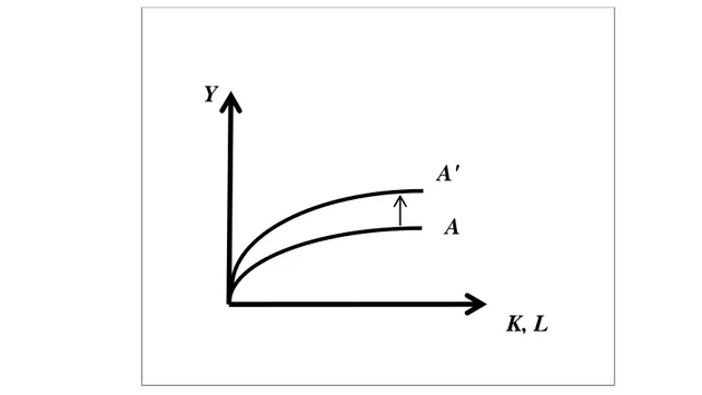
Technical progress influences the curve of the production. If the variation of technology is positive, the curve shifts upward, as shown in the picture below (Figure 2), so that the value of output is higher. Vice versa, with a negative variation of technology the curve would move downward determining a lower amount of production.

Figure 7. Variation of Technology

Q

L

f (K,L

)

Q

L

f (K,L)

f' (K,L)

(26)

The marginal product (MP) of a factor is determined by the change in output from a small input variation, holding constant the use of all the other production factors:

𝑀𝑃_𝐿= ∆𝑄 ∆𝐿

(3)

If we look with a broader perspective and a longer time horizon, the considerations on the production and change its function. In the long run, in fact, all inputs are variable. The combinations of inputs that guarantee the same level of output represents an isoquant. A map of isoquants represents a set of isoquants curves, each of which corresponds to a constant level of product. Moving from the intersection of the axis the output increases, as we can see in the picture below.

Figure 8. Map of Isoquants

In the long run we can introduce an important ratio, which is the marginal rate of technical substitution, that measures the additional quantity of a production factor required by the firm to continue to produce the same amount of output, as a result of the reduction of the second production factor. In other words, you can replace a factor with another, without changing the production at the rate.

The marginal rate of technical substitution is equal to the ratio of the marginal productivity of factors of production or the absolute value of the slope of the isoquant:

𝑀𝑅𝑆𝑇 = 𝑀𝑃𝐿 𝑀𝑃_𝐾 = | ∆𝐾 ∆𝐿| (4) Labour (L) Capital (K) Increasing Output 𝑄1 𝑄2 𝑄3

(27)

In the long run it is useful to introduce also the concept of returns to scale. They are tied to changes in proportion of all production factors, which take place simultaneously. The returns to scale are a key factor in determining the structure of a firm. Following an increase of production factors, the returns to scale can be increasing, constant or decreasing. It is observed that the decreasing returns to scale have nothing to do with the law of decreasing marginal returns. The marginal product of the individual factors should be decreasing, but the production function can have decreasing, constant or increasing returns to scale.

Speaking of production and productive system of a country inevitably, we have to introduce the concept of GDP, or gross domestic product, a key variable of macroeconomics. GDP is the market value of all final goods and services produced in a country in a given period. We can clarify the various terms that come into this definition:

 Gross: indicates the value of production before amortization, i.e. the natural depreciation of the physical capital stock occurred during the period.

 Market value: goods and services entering GDP are valuated at market (current) prices, i.e. the prices at which they are effectively sold.

 All: less than those produced and sold illegally; less than those produced and consumed within households.

 Final: the flour is a final good if sold as flour; it is an intermediated good if it is sold to the baker to make bread. In this case, the value of the flour is incorporated in the value of the bread.

 Product: GDP measures the value of goods and services produced in a year, not the transactions in a year; so new cars that are bought and sold are part of GDP, as produced in the year, while the used car market is not recorded in the GDP.

 In a country: GDP measures what is produced in Italy, not what is produced by Italians. Italians can produce abroad; while in Italy can also produce foreign people. GDP includes what is produced by foreign people in Italy and excludes that which is produced abroad by Italian.

 Period: the time horizon taken in consideration is the year.

There are different ways to calculate GDP, such as the value-added method, the income approach and the expenditure method. Although GDP has more specific characteristics, we give the following synthetic formulation:

(28)

With Y we indicate the GDP, C is the private consumption, I is the expenditure for private investment in durable goods including changes in stocks, G is the public expenditure and X are the net exports (E – Z, where E are the exports and Z the imports). GDP has a leading position about his ability to express or symbolize the well-being of a national community and its level of development or progress. However, GDP is not the only macroeconomic measure of product or income. As already mentioned it includes income earned in a country (Italy, for example) by foreign residents but excludes the incomes of Italian citizens but earned abroad. If we add to GDP the net income from abroad, that is, the balance between incomes of Italian citizens abroad and foreign income in Italy, we get the Gross National Product or GNP:

GNP = GDP + net income from abroad

In large countries, like the US or the European Union the difference between GDP and GNP is minimal (3% - 4%), because the incomes of residents abroad are very similar to that of the foreign income dimension to inside of these countries. For smaller countries, the two values can be very different. Consider the case of countries with high emigration and low immigration, where there are few foreign firms, which establish their facilities there. For similar countries will have a larger GNP than GDP. Conversely, countries with significant immigration and a strong ability to attract foreign companies will have a much greater GDP of GNP.

There are many other indices and measures of well-being and production for a country, but none of them has been so far able to be absolute and irreplaceable, so in the general common accounting of the countries, nowadays, it usually speaks of GDP. The production and the GDP are fundamental to give us information about the output growth of a country. From a macroeconomic point of view, the three main dimensions of aggregate economic activity are output growth, the unemployment rate, and the inflation rate. Clearly, they are not independent, so in the following paragraphs we will analyze the latter two in order to have a complete scheme of study.

When economists want to dig deeper and to look at the state of health of a country, they look at three basic variables. The output growth, which is the rate of change of output. The unemployment rate, which is the proportion of workers in the economy who are not employed and are looking for a job. The inflation rate, the rate at which the average price of the goods in the economy is increasing over time. Therefore, we will analyse separately also the last two variables.

1.6 The Unemployment Rate

Because it is a measure of aggregate activity, GDP is obviously the most important macroeconomic variable. However, two other variables, which are unemployment and inflation, tell us about other important aspects of how an economy is performing. We will use these variables, together with the technological progress to

(29)

construct our model in the last chapter of this project. This paragraph focuses on the unemployment rate.

We start with two definitions. Employment is the number of people who have a job. Unemployment is the number of people who do not have a job but are looking for one. The labour force is the sum of employment and unemployment:

𝐿 = 𝑁 + 𝑈 (6)

where 𝐿 is the labour force, 𝑁 is the employment and 𝑈 is the unemployment. The unemployment rate is the ratio of the number of people who are unemployed to the number of people in the labor force:

𝑢 =𝑈 𝐿

(7)

where 𝑢 is the unemployment rate. Determining whether somebody is unemployed is harder. Recall from the definition that, to be classified as unemployed, a person must meet two conditions: that he or she does not have a job, and he or she is looking for one; this second condition is harder to assess.

Until the 1940s in the United States, and until more recently in most other countries, the only available source of data on unemployment was the number of people registered at unemployment offices, and so only those workers who were registered in unemployment offices were counted as unemployed. This system led to a poor measure of unemployment. How many of those looking for jobs actually registered at the unemployment office varied both across countries and across time. Those who had no incentive to register, for example, those who had exhausted their unemployment benefits, were unlikely to take the time to come to the unemployment office, so they were not counted. Countries with less generous benefit systems were likely to have fewer unemployed registering, and therefore smaller measured unemployment rates. Today, most rich countries rely on large surveys of households to compute the unemployment rate. In the United States, this survey is called the Current Population Survey (CPS). It relies on interviews of 50,000 households every month. The survey classifies a person as employed if he or she has a job at the time of the interview; it classifies a person as unemployed if he or she does not have a job and has been looking for a job in the last four weeks. Most other countries use a similar definition of unemployment. Note that only those looking for a job are counted as unemployed; those who do not have a job and are not looking for one are counted as not in the labor force. When unemployment is high, some of the unemployed give up looking for a job and therefore are no longer counted as unemployed. These people are known as discouraged workers. Take an extreme example: if all workers without a job gave up looking for one, the unemployment rate would equal zero. This would make the unemployment rate a very poor indicator of what is happening in the labor market. This example is too extreme; in practice, when the economy slows down, we typically observe both an increase in unemployment and an increase in the number of people who drop out of the labor force. Equivalently, a higher unemployment

(30)

rate is typically associated with a lower participation rate, defined as the ratio of the labor force to the total population of working age.

Economists care about unemployment for two reasons. First, they care about unemployment because of its direct effect on the welfare of the unemployed. Although unemployment benefits are more generous today than they were during the Great Depression, unemployment is still often associated with financial and psychological suffering. How much suffering depends on the nature of the unemployment. One image of unemployment is that of a stagnant pool, of people remaining unemployed for long periods. In normal times, in the United States, this image is not right. Every month, many people become unemployed, and many of the unemployed find jobs. When unemployment increases, however, as is the case now, the image becomes more accurate. Not only are more people unemployed, but also many of them are unemployed for a long time. In short, when the unemployment increases, not only does unemployment become both more widespread, but it also becomes more painful. Second, economists also care about the unemployment rate because it provides a signal that the economy may not be using some of its resources efficiently. Many workers who want to work do not find jobs; the economy is not utilizing its human resources efficiently. From this viewpoint, can very low unemployment also be a problem? The answer is yes. Like an engine running at too high a speed, an economy in which unemployment is very low may be over utilizing its resources and run into labor shortages. How low is “too low”? This is a difficult question. The question came up at the beginning of the new millennium in the United States. At the end of 2000, some economists worried that the unemployment rate, 4% at the time, was indeed too low. So, while they did not advocate triggering a recession, they favored lower (but positive) output growth for some time, to allow the unemployment rate to increase to a somewhat higher level. It turned out that they got more than they had asked for a recession rather than a slowdown.

Let us see what has been the trend of unemployment in Europe, in order to understand also the other economic phenomena, which are correlated.

(31)

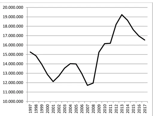
Figure 9. Euro-Area Total Unemployment, Member States

Figure 9 shows the trend of the Total Unemployment in the Euro Area in a period from 1997 until nowadays. The values are always above eleven millions of persons and under fifteen millions from the beginning until 2009. In 2008, indeed, with the outbreak of the global financial crisis, they begin to rise sharply. From 2010 to 2011, the trend seems to be quite stable around a value of sixteen millions, but from 2011, it increases again until the highest value of more than nineteen millions in 2014. In the last three years, the trend is decreasing, even if the values are always high and far from the values of the pre-crisis period.

1.7 The Inflation Rate

As we said before the other important variable for an economy is the Inflation Rate, let us see what are its main features.

Inflation is a sustained rise in the general level of prices, the price level. The inflation rate is the rate at which the price level increases (symmetrically, deflation is a sustained decline in the price level; it corresponds to a negative inflation rate). The practical issue is how to define the price level so that the inflation rate can be measured. Macroeconomists typically look at two measures of the price level, at two price indexes: the GDP deflator and the Consumer Price Index. If a higher inflation rate meant just a faster but proportional increase in all prices and wages, a case called pure inflation, inflation would be only a minor inconvenience, as relative prices would be unaffected. Take, for example, the workers’ real wage, the wage measured in terms of goods rather than in dollars. In an economy with 10% more inflation, prices would increase by 10% more a year. However, wages would also increase by 10% more a year, so real wages

10.000.000 11.000.000 12.000.000 13.000.000 14.000.000 15.000.000 16.000.000 17.000.000 18.000.000 19.000.000 20.000.000 19 97 19 98 19 99 20 00 20 01 20 02 20 03 20 04 20 05 20 06 20 07 20 08 20 09 20 10 20 11 20 12 20 13 20 14 20 15 20 16 20 17