View of On a Test of Hypothesis to Verify the Operating Risk Due to Accountancy Errors

Paola M. Chiodini

Dipartimento di Statistica e Metodi Quantitativi, Università degli Studi di Milano – Bicocca, Via Bicocca degli Arcimboldi 8, 20126 Milano, Italia

Silvia Facchinetti

Dipartimento di Scienze Statistiche, Università Cattolica del S. Cuore, Largo Gemelli 1, 20123 Milano, Italia

1. I

NTRODUCTION AND BACKGROUND

In the last years the decision making process had to face a growing “dynamism” of the events: market changes, the use of technical innovations and communication means, industry specializations, which lead to follow the different operations made by the firm, to underline the irregularities that can generate crisis, economic losses or reductions in market share (Chiodini and Magagnoli, 2004; Low, 2004).

Internal control includes systematic measures adopted by an organization to conduct business in an efficient manner, to safeguard assets and resources, to check the accuracy and reliability of the accounting data, to promote operative efficiency, to produce reliable and timely financial and management informations, to encourage adherence to prescribed managerial policies and to detect errors and frauds. Therefore, a system of internal control extends beyond the matters which relate directly to the functions of the accounting and financial departments. Generally, controls can be of three types: a preventive control, designed to discourage from occurring errors or irregularities; a corrective control, designed to correct errors or irregularities that have been detected; a detective control, designed to find errors or irregularities after they have occurred (Guy et al., 2002).

The demands of the firms of a control extended to all phases of its organization have led to a wide use of statistical analysis procedures in order to locate the system irregularities, to assess the market and to take operational and strategic decisions in conditions of uncertainty (Ashton and Ashton, 1988; Kriens and Veenstra 1985).

The aim of this study is to examine a new suitable procedure for internal auditing in order to define the error risk that could imply distortions and wrong decisions by the management. The audit system develops in different steps: some are not susceptible to sampling procedures, while others may be held using sampling techniques. In usual sampling techniques adopted in auditing, sampling plans are used to estimate the amount of the accountancy during time (i.e. one year), with an inference about the series of transactions that is assumed as the “statistical population” (Arens and Loebbecke, 1981; Smith 1976). Such assumption is denoted “static” or “ex post”. In this study the same informations are used to follow the data development during time (Brown and Rozeff, 1979; Caprara, 1988) and to estimate their behaviour from a “dynamic” point of view. In particular, we introduce a statistical test of hypothesis and irregularity signal, that can be connected with the ones applied in the production processes known as “control charts”.

the occurrence of assignable causes or process shifts so that investigation of the process and corrective actions may be undertaken (Montgomery, 2005; Kanji,2004). Control charts are used to monitor a process for some quality characteristic that can be measured and expressed numerically such as thickness, weight and defective fractions (control charts for variables) or that are attributes and expressed categorically, for example “conforming” or conforming”, “defective” or “non-defective” (control charts for attributes).

In auditing, both internal and external, the concept of risk is very complex (Teitlebaum and Robinson, 1975; Libby et al., 1985; Houston et al., 1999; Cleary and Thibodeau, 2005), with reference to the different kinds of fraud and acceptability that have a degree of subjectivity. For a review on statistical fraud detections see Bolton and Hand (2002). Therefore the study assumes as risk measure the probability of “no signal” when some irregularities are happening and hence in terms of the probability of the second type

β

in function of the shift of the accountancy from the standard conditions. This represents the probability to not report a situation of irregularity in the accounts in the event of removal of the accounting process and therefore it is considered right in terms of regularity. The aim is to monitor the possibility of intervening with a comprehensive analysis of the accounts when it does not meet the conditions required under the null hypothesis (regularity of the accounting entries) and to reduce the probability of not reporting a situation of irregularity in the accounts in terms of number of transactions affected by errors in the sample that overcome a given threshold (natural error rate), and the mean amount of monetary errors found in incorrect records. Therefore we compute a mixed structure, for variables and for attribute different on the standard control procedure.

The paper is organized as follows. The next section explains the marginal and the joint test of hypotheses to verify the regularity of the accounting system. In section 3 the decisional procedure consisting of two hypothesis systems is proposed. In particular, the first system is referred to the analysis of the first marginal test of hypothesis relative to the frequency of accounting errors

p

, with particular attention to the differences between non-randomized or randomized test. While the second system is referred to the analysis of the second marginal test of hypothesis relative to the mean (or median) of the book errors conditioned from the first one. Here the distinction is between unilateral and bilateral test. Moreover, the joint operative characteristic function of the test is calculated. Defined the decision-making procedure that allows to accept or reject the null hypothesis, in section 4, a sensitivity analysis of the procedure is described. Finally, in section 5 some future developments are presented.

2. M

ODEL AND TEST OF HYPOTHESES

Within the audit accounting, the risk concept is highly complex and difficult to apply in relation to different types of possible frauds and to their acceptability degree.

The given check procedure is a multiple test of hypothesis, iteratively applied to the accountancy records that belongs to homogeneous classes and related to a short time

t

I

= − ∆

(

t

t t

,

]

, with

∆ =

t 1

, (i.e.: one day), where for the

N

_t accountancy records available,

t

n

of them are analysed.

In audit context two quantitative elements play a role of particular interest. The frequency of a book error

p

and the mean (or median)

θ

_L of the conditional distribution of the error random variable

X Vc Vr

=

–

, given by the difference between the real book value

Vc

and the recorded value

Vr

, that follows a known law

F x; ,

(

θ θ

_{L D}

)

depending on a location parameter

θ

_L and on

a dispersion parameter

θ

_D (that is considered constant).

In other words, we can refer to the following two systems of hypotheses:

1. a system referred to the frequency of accounting errors

p

,

X 0

≠

or

(

X

+

_>

0,

X

−

_<

0

)

_{, in} t

I

period:

H p p

H p p

' 0 0 ' 1 0

:

:



≤





>



(1)

and we accept the null hypotheses if the error fraction

p

is below the value

p

₀ (few errors); 2. a system referred to the mean (or median) of the book errors,

X 0

≠

or

(

X

+

_>

0,

X

−

_<

0

)

_{, in}

t

I

period. This may be unilateral, by checking the only positive (or negative) errors:

L L L L

H

H

" 0 0 " 1 0

:

:

θ

θ

θ

θ



≤





>



(2)

and we accept the null hypotheses if the mean value of the accountancy errors

θ

_L is below the value

θ

_L0 (small errors); or bilateral, by checking the presence of errors both positive and negative

L L L L

H

H

" 0 0 " 1 0

:

:

θ

θ

θ

θ



≤





>



(3)

The values

p

₀ and

θ

_L0 are boundary values in the acceptable conditions of the accounting. The operative choice of these values depends on the sample size that is linked to the number of the observed units

N

in the considered period of time and on the significance level

α

.

Consequently it is possible to set up a complex system of hypotheses to verify the regularity of the accounting system when

p p

≤

₀ or

θ

_L

≤

θ

_L0 or of the both, in the situation of the unilateral test.

Then the joint system of hypotheses is









>

∨

>

≤

∧

≤

0 0 1 0 0 0 L L L L

p

p

:

H

p

p

:

H

θ

θ

θ

θ

(4) and similarly in the situation of the bilateral test.

3. T

HE DECISIONAL PROCEDURE

As said before, the proposed procedure consists of two hypothesis systems. The first system regards the verify of the presence of units characterised by accounting errors, the second one is about the verification of the mean (or median) value on the observed non correct units

r

. In other words, the second hypothesis system is conditioned to the first one.

form the hypothesis

H

₀ of the system (4), we have to formalize the decisional rules belonging to each single hypothesis, so that to have a unique decisional rule

D

₀ to accept the null hypothesis obtained as the intersection of the two marginal decisional rules.

3.1.

The first test of hypothesis

In the test of hypothesis (1) we verify the presence of units characterised by book errors.

Let consider a simple random sample of size

n

(with

n

<<

N

), and let

r

be the number of units characterised by a book error in the sample. The number

r

is assumed distributed as a Poisson random variable with parameter

λ

=

np

(considering acceptable the conditions of the asymptotic approximation of hypergeometric and binomial distribution to the Poisson distribution). The hypothesis system (1) becomes









>

≤

→









>

≤

0 1 0 0 0 1 0 0

λ

λ

λ

λ

:

H

:

H

p

p

:

H

p

p

:

H

' ' ' ' (5) where

λ

₀

=

np

₀.

The test may be non-randomized or randomized.

NON-RANDOMIZED TEST. If we consider a non-randomized test, the critical function to reject the

null hypothesis is

( )











→

>

→

≤

=

Ψ

_' c ' c '

D

decision

r

r

if

D

decision

r

r

if

;

r

1 0

1

0

λ

where the critical value

r

_c depends on the significance level of the first test

α

' and

D

'

0 is the acceptance of H'

0 while

D

1' is the acceptance of

H

1', respectively.

Let

g r ;

(

λ

)

be the probability distribution function and

G r ;

(

λ

)

the cumulative distribution function of a Poisson random variable, respectively. We have

(

c

)

(

c

)

G r

'

G r

0 0

1;

λ

1

α

;

λ

−

< −

≤

so that:

(

c

) (

c

)

(

c

)

G r

g r

'

G r

0 0 0

;

λ

−

;

λ

< −

1

α

≤

;

λ

This equation allows, assigned

α

' and

λ

₀, to obtain the critical value

r

_c of the procedure. In this case, the real significance level is equal to:

(

c

)

G r

' '

*

1

;

0

α

= −



_

λ



_

<

α

0

λ λ

>

gives the probability of the second type error for the hypothesis system (1)

Π

'

( )

λ

is the power function of the test). This function, for assigned values of

n

,

α

' and

p

₀ (from which

r

_c

derived), can be expressed as a function of

λ

=

np n p

=

(

₀

+ ∆

)

, where

∆

is the distance from

p

to

p

₀. So we have

( )

rc

( )

(

)

c r

g r

G r

' 0

;

;

β λ

λ

λ

=

=

∑

=

In particular, for

λ λ

=

₀ and so

∆ =

0

,

_{β λ}

'

( )

_≡

_β

'

(

_∆

_,

n

)

_{, we have}

( )

(

) (

)

' ' '

0

1

*

1

β λ

= −

α

≥ −

α

RANDOMIZED TEST. As the non-randomized test does not have an exact significant level equal

to

α

' we consider a randomized test. In this case the critical function to reject the null hypothesis is

( )

cc c

if r r

r

if r r

if r r

'

0

;

1

λ

ψ

<





Ψ

=

_

=

 >



,

where

(

)

(

)

(

)

(

)

c c c

G r

g r

g r

' _{' '} 0 _* 0 0

;

1

;

;

λ

α

_{α α}

ψ

λ

λ

− −

₋

=

=

is the randomness probability of the decisional procedure for

r r

=

_c.

We observe that for

λ λ

=

₀ he expected value of the random variable

_Ψ

'

( )

r

_;

_λ

_is

_α

'_:

(

)

{

}

{

}

{

}

{

}

(

)

(

)

(

)

(

)

(

(

)

)

(

)

(

)

(

)

c c c c c c c c c

E

r

P r r

P r r

P r r

G r

g r

G r

g r

G r

G r

' 0 ' 0 0 0 0 ' ' 0 0

;

0

1

;

1

;

1

;

;

;

1

1

;

λ

ψ

λ

α

λ

λ

λ

λ

α

λ

α

Ψ

= ⋅

<

+ ⋅

=

+ ⋅

>

=

− −

=

+ −

=



_{ }

_

=

_

− −

_

+ −

_

_

=

.

The function

E

_{

_Ψ

'

( )

r

_;

_λ

_}

_{, considered as function of}

_λ

_{, is the power function of the test.}

( )

rc

( )

(

)

c r

g r

g r

' 0

;

;

β λ

λ ψ

λ

=

=

∑

− ⋅

.

In particular, for

λ λ

=

₀ and so

∆

=0

, '

( )

'

(

n p

)

0

, ,

β λ

≡

β

∆

, we have

( )

(

)

' ' 0

1

β λ

= −

α

.

3.2.

The second test of hypothesis

In the situation of non-systematic absence of abnormal behavior in the recording of the book values, the assumption of normal distribution of the accounting error is justifiable both from theoretical and applicative point of view. Moreover, because in this context it makes no sense to consider small sample sizes, considering the sample mean as test statistic the assumption of normality is approximately (for the central limit theorem) even if the assumption of normal distribution for X is removed. Consequently the unilateral and bilateral hypotheses systems of the second test of hypothesis regards the random variable

X N µ

2

0

,

(

σ

)



, with

σ

₀2 assigned on the basis of the experience.

The verification of the mean value is conducted on the observed units

r

characterised by a book error in the sample. In other words, the second hypothesis system is conditioned to the first one. In fact it is taken into account only if it was observed in the first test

r

∈

[ ]

1,

r

_c .

The test may be unilateral or bilateral.

UNILATERAL TEST. If we consider the unilateral hypotheses systems with

i

x

> =

0;

i

1, 2, ,

…

r

, the decisional rule to accept the null hypothesis is

c c

D x x

D x x

'' 0 '' 1

:

:



≤





>



where

x

=

∑

_ir₌₁

x r

_i

/

is the sample mean and

x

_c is the critical value obtained from the significance level

α

'': c

x

z

r

'' 0 0 1α

σ

µ

₋

=

+

.

As known,

z

_1−α'' is the percentage point

(

1

−

α

'

)

100

of the standard normal distribution

variable such that

φ

(

z

_1−α''

)

= −

1

α

'', where

φ

is the cumulative distribution function of the

standard normal distribution.

Considering the standardized parameter

δ

=

µ µ

(

−

₀

)

/

σ

₀ with

δ

≥

0

instead of

µ µ

>

₀, the characteristic function of the test is

( )

r

P D

{

}

( )

r

(

z

''

r

)

'' '' ''

0 0 0 ₁

;

:

1

;

_α

β δ

=

µ µ δσ

=

+

= − Π

δ

=

φ

₋

−

δ

.

(6) For

δ

=0

, such function takes the value

_β

''

( )

_0;

_{= −}

r

₁

_α

''_{, and for}

_δ

_{→ ∞}

_,

(

)

lim

''

_;

r

₀

δ→ ∞

β δ

=

.

The function

φ

( )

z

can be approximated to zero for

z -4

≤

, so we can limit the determination of the function

_{β δ}

''

(

_;

r

)

_{for values}

_z

_r

''

1

, 4

)

0

(

(

_α

)

/

δ

∈

+

₋ . For example, for

''

_5%

α

=

and

r 9

=

we have

δ

∈ ≈

(

0, 2

)

.

BILATERAL TEST. If we consider the bilateral case, the hypotheses systems can be write as:

(

) (

)

H

H

for

H

H

'' '' 0 0 0 0 0 0 '' '' 1 0 0 1 0

:

:

0

:

:

µ µ

µ

µ µ

µ

µ

µ

µ µ

µ µ



≤



−

≤ ≤



_→



_≥





< −

∪

>

>

_







The decisional rule based on the sample mean of the r observations

x

_i

≠

0

;

i

=

1, 2,

…

, r

, is

(

c

) (

c

)

c c c

D

x

x x

for x

D

x

x

x x

'' 0 '' 1

:

0

:



− ≤ ≤



_>



< −

∪

>



To determine the critical value

x

_c, we consider

µ µ

=

₀ and

α

''

(

<

0.5

)

such that

L U '' '' ''

α

=

α

+

α

where

P X

{

_{< −}

x

_c

}

₌

_α

_L'' _and

{

}

c U

P X x

_>

₌

_α

'' _with L U ''

_,

''

₀

α α

≥

. Being for hypothesis

X N

(

2

r

)

0

,

0

/

µ σ

≈

, we have

(

)

(

)

(

)

(

)

L U L L U U c L c c c c U

z

z

x

_r

z

x

x

r

_r

r

x

_z

_x

z

z

r

_r

'' '' '' '' '' '' '' 0 ₀ 1 1 0 1 0 0 '' 0 _{1 1} 0 0 1 ₀ 0 0

1

2

1

2

α α α α α α

µ

_σ

α

ϕ

_µ

σ

σ

µ

_µ

_σ

α

ϕ

_σ

_µ

σ

− − − − − −





_{= −}



+





_

+













=

+

_

=





_{ →}



_→











−



−



_{= − }



₌

₋









_



_



_



=



_

(7)

The values

α

_L'' and

α

_U'' derive from the second equations of the system (7) using the relation:

L U

r

z

₁ ''

z

₁ '' ₀ 0

2

α α

_σ

µ

−

−

−

=

where L

z

_1−α'' and U

z

_1−α'' are the percentage points

(

1

−

α

_L''

)

100

and

(

1

−

α

_U''

)

100

of the standard

normal distribution.

From the previous equations it is possible to determine the critical value

x

_c for

µ

₀

≥

0

. In particular, for

µ

₀

=

0

we have

/ 2

α

_L''

=

α

_U''

=

α

'' and so:

c

x

z

r

" 0 1 α/2

σ

−

=

.

The function

φ

( )

z

can be approximated to one for

z 4

≥

, so the relation

(

c

)

L

r

x

" 0 0

1

φ

µ

α

σ





+

= −









for

(

c

)

r

x

₀ 0

4

µ

σ

+

≥

implies

1

−

α

L''

≅

1

and so

α

L''

≅

0

and U'' ''

α

≅

α

. If

z

r

'' 1 0 0

4

2

α

σ

µ

_≥



−

−















, the approximate critical value is

x

c

r

z

''

0 0 1 α

σ

µ

₋

=

+

. In such case c

x

is the same of the unilateral case.

If

z

r

'' 1 0 0

4

0

2

α

σ

µ



−

−



<

<



_



_





we have to calculate L U ''

_,

''

α α

, and

x

_c using the equations (7). Once defined

x

_c, we can calculate the operative characteristic function of the conditioned test:

( )

r

P X

{

x

c

}

''

0 0

;

:

β δ

=

≤

µ δσ

+

where the mean of the random variable

X

is indicated as

µ µ

=

₀

+

δσ

₀ with

δ

≥

0

. As

E X

{ }

=

µ δσ

₀

+

₀ and

Var X

{ }

2

r

0

/

σ

=

, we have

( )

r

(

z

_U''

r

) (

z

_L''

r

) (

z

_U''

r

) (

z

'' _U''

r

)

'' 1 1

;

_{α α α α α}

β δ

=

φ

₋

−

δ

−

φ

−

δ

=

φ

₋

−

δ

−

φ

₋

−

δ

(8)

For a fixed value

α

'' this is a monotonically increasing function with respect to

δ

and

r

. In particular, for

δ

=

0

:

( )

r

( ) ( )

z

_U''

z

_L'' U L

( )

r

'' '' '' '' '' '' 1

0;

_{α α}

1

1

0;

β

=

φ

₋

−

φ

= −

α

−

α

= −

α

→ Π

=

α

As noted before, if

µ

₀

=

0

we have

/ 2

α

_L''

=

α

_U''

=

α

'' , so:

( )

r

(

z

''

r

) (

z

''

r

)

'' 1 /2 /2

;

_{α α}

β δ

=

φ

₋

−

δ

−

φ

−

δ

(9) For         − ≥ − 2 4 ₁ 0 0 '' z r α σ

µ we have αL'' ≅0 and αU'' ≅α'', consequently

( )

r

(

z

''

r

)

''

1

;

_α

β δ

=

φ

₋

−

δ

(10)

and the approximation of the unilateral case (6) is still valid.

As indicated in the preceding paragraphs it is possible to use as location index the median (or another quantile point) as an alternative to the mean. The benefit would be that these indexes are robust. This property is especially useful when we suspect that some modalities very large or very

small are abnormal.

In this way it would be possible to use a non-parametric version of the procedure that does not require the assumption of normality of the data.

3.3.

The joint operative characteristic function

We now define the joint operative characteristic function

β

(

∆

;

δ

)

, where

∆

is the distance from

p

to

p

₀ (first systems of hypotheses), and

δ

=

(

µ µ

−

₀

)

/

σ

₀ (second systems of hypotheses), for the cases examined in sections 3.1 and 3.2.

NON-RANDOMIZED TEST. If we consider the unilateral and non-randomized test, the joint

operative characteristic function is:

(

)

(

)

(

)

rc

(

) (

)

r

P D

g r

g r

''

r

0 1

;

: ,

0;

;

;

β

δ

δ

λ

λ β δ

=

∆ =

∆ =

= +

∑

(11)

where

_{β δ}

''

( )

_;

r

_for

_δ

_≥

₀

_{is defined in equation (6).}

We precise that if

r 0

=

we accept the null hypothesis of the joint test of hypotheses, while for

r r

>

_c we refuse it. For

1 < <

r r

_c the decision derives from the second test (see paragraph 3.2). For the bilateral and non-randomized test, we consider in the previous equation defined in equation (8).

We observe that for

∆ =

0

and

δ

=

0

we have

( )

(

)

(

) ( )

(

)

(

)

(

)

(

)

(

)

(

)

(

)

(

)(

)

(

)

c c c r r r r r r

g r

np

g r

r

g

g r

g

g r

g

g

'' 0 0 0 1 '' '' 0 0 0 1 '' '' 0 0 0 '' ' '' * 0

0;0

0;

;

0;

0;

1

;

0;

1

;

0;

1

1

0;

1

β

λ

λ β

λ

α

λ

α

λ

α

λ

α

λ

α

α

α

λ

α

= = =

=

= =

+

=

=

+ −

±

=

= −

+

=

= −

−

+

= −

∑

∑

∑

(12)

where

α

is the exact significance level of the joint test of hypothesis.

In equation (12)

_β

''

(

_0;

r

)

_{= −}

₁

_α

''_,

_g

(

)

_e

0

_e

np0 0

0;

λ

₌

−λ

₌

− _and

(

)

c r r

g r

' ' 0 * 0

;

λ

1

α

1

α

=

= −

≥ −

∑

, so

(

'

)(

''

)

(

' ''

)

' ''

(

' ''

)

(

'

g

(

)

)

'' * * * * * 0

1

−

α

1

−

α

= −

1

α α

+

+

α α

> − → ≅

1

α

α

α α

+

−

α

+

0;

λ α

If we do not consider the term

(

'

g

(

)

)

''

*

0;

0

α

+

λ α

, we obtain

(

' ''

)

' ''

* α α α

α

α= + ≤ + .

Operatively, we can proceed by assigning a small value to α (1%, 5%, 10%) and build the test

RANDOMIZED TEST. If we consider the procedure of the first system of hypothesis using a randomized test, the joint operative characteristic function of the test

β

(

∆

;

δ

)

can be written as

(

)

(

)

( ) ( ) (

) (

) (

)

(

)

( ) ( )

(

) (

)

c c r c c r r c c r

g

g r

r

g r

r

g

g r

r

g r

r

1 '' '' 1 '' '' 1

;

0;

;

;

1

;

;

0;

;

;

;

;

.

β

δ

λ

λ β δ

ψ

λ β δ

λ

λ β δ

ψ

λ β δ

− = =

∆ =

+

+ −

=

=

+

−

∑

∑

(13)

We note that for

∆ =

0

and

δ

=

0

we have

( )

(

)

(

) ( )

(

) (

)

(

)

(

)

(

)

(

)

(

)

(

)

(

)

(

)

(

)

(

)

(

)(

)

c c c r c c r r c r r c r

g

g r

r

g r

r

g

g r

g r

g

g r

g r

g

g

'' '' 0 0 0 1 '' '' '' 0 0 0 0 1 '' '' 0 0 0 0 ' '' ''

0; 0

0;

;

0;

;

0;

0;

;

1

;

1

0;

1

;

;

0;

1

1

0;

β

λ

λ β

ψ

λ β

λ

λ

α

ψ

λ

α

α

λ

α

λ

ψ

λ

α

λ

α

α

α

= = =

=

+

−

=

=

+

−

−

−

±

=





= −

_

−

_

+

=





= −

−

+

∑

∑

∑

(

λ

0

)

= −

1

α

(14) where

_β

''

(

_0;

r

)

_{= −}

₁

_α

''_,

_g

(

)

_e

0

_e

np0 0

0;

λ

₌

−λ

₌

− _and rc

(

)

(

)

c r

g r

g r

' 0 0 0

;

λ

ψ

;

λ

1

α

=

−

= −

∑

.

We may observe that in equations (11), (12), (13) and (14) the terms

g

(

0;

λ

₀

)

or

g 0;

(

λ

)

can be disregarded if

λ

₀ or

λ

are greater than 7, as their contribution would be lower than 0,001. In this way to consider the joint procedure is equivalent to consider the two joint tests stochastically independent.

4. S

ENSITIVITY ANALYSIS OF THE PROCEDURE

Defined the decision-making procedure that allows on the basis of sample data to accept or reject the null hypothesis using the critical values (

r

_c and

x

_c), consistent with the level of quality required for the correctness accounting and in accordance with the parameters (

p

₀ and

µ

₀ ) and significance levels of the two tests (

α

' and

α

''), it is interesting to evaluate the level of risk considered acceptable in a real situation incompatible with the null hypothesis in terms of probabilities. This probability is expressed by the operational characteristic function

β

(

∆

;

δ

)

where

δ

and

∆

are appropriate measures of the distances of the real values from the parameters

p

and

µ

from

p

₀ and

µ

₀. This function is called the "risk of error in the decision-making procedure sample" and is an indicator of general use for the choice of parameters that establish the decision-making procedure. It has to be noted that it also depends on the type of procedure of randomness (random or non-random) as regards the first test, and on the type of hypothesis (unilateral or bilateral) as regards the second test, conditional on the first.

to direct operatively the conductors of the investigation of auditing in the choice of the parameters, the next Table 1 presents the critical values

r

_c, the real significance level of the first test

α

_*' and the randomness probability

ψ

of the decisional procedure for

r r

=

_c. In particular we have referred to:

n

=

100, 250, 500

;

p

₀

=

0.01, 0.05, 0.10

and

α

'

=

1%, 2.5%, 5%

.

TABLE 1

Critical valuesr_c, real significance level α_*' and randomness probability ψ of the decisional procedure for

c r=r . ' 1% α = _{α =}' _{2.5% α =}' _5% n p₀ λ₀ g(0; )λ₀ r _c '

( )

* % α ψ r c α*'

( )

% ψ r c α*'

( )

% ψ 0.01 1.0 0.3679 4 0.37 0.4136 3 1.9.0 0.0981 3 1.90 0.5058 100 0.05 5.0 0.0067 11 0.55 0.5517 10 1.37 0.6234 9 3.18 0.5011 0.10 10.0 ~0 18 0.72 0.3968 17 1.43 0.84 15 4.87 0.0363 0.01 2.5 0.0821 7 0.42 0.5788 6 1.42 0.3885 5 4.20 0.1194 250 0.05 12.5 ~0 21 0.94 0.0759 20 1.73 0.5789 19 3.06 0.9129 0.10 25.0 ~0 37 0.92 0.1478 35 2.25 0.2233 33 4.98 0.0101 0.01 5.0 0.0067 11 0.55 0.5517 10 1.37 0.6234 9 3.18 0.5011 500 0.05 25.0 ~0 37 0.92 0.1478 35 2.25 0.2233 33 4.98 0.0101 0.10 50.0 ~0 67 0.89 0.3128 64 2.36 0.1695 62 4.24 0.5725 In the Table 1 we observe that the values of the function

g

(

0;

λ

₀

)

show the probability that there are no accounting errors. Considering the critical values

r

_c we observe that in some situations such values are very small and, therefore, the means calculated at the second test result lacking in precision. In particular, already for the smallest value of α ='

( )

1% in some situations we observe values of

r

_c very small (i.e. 4, 7, 11) and decreasing when

α

' increases. To have sense the use of the test on the mean you need to consider combinations of

p

₀ and

n

such that ensure a value of

λ

₀

=

np

₀

≥

10

.

Moreover the real significance level of the first test

α

_*' is that of the case of non-randomized test:

α

_*'

<

α

', while for the randomized test is equal to the nominal level

α

'.

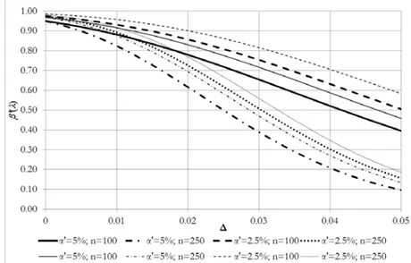
To complete the observations arising from Table 1, the Figure 1 presents the probability to accept the null hypothesis of the first test (operative characteristic function) as a function of

∆

for the randomized and non-randomized test. In particular we have referred to:

p

₀

=

0.05;

=

n

100, 250

and α'

α

'

=

2.5%, 5%

. We note that in the graph the thick lines are

Figure 1 – Probability to accept the null hypothesis of the first test for the randomized (thick lines) and non-randomized (fine lines) test.

The figure shows that the risk function is very sensitive to sample size. In particular, it is much more sensitive the higher is the value of

n

. It is generally argued that the test presents a good discriminating ability.

Once defined the conditions of the first test about the frequency of accounting errors

p

, it is possible to carry out the second one relative to the mean of those errors. We emphasize that the second test is conditioned to the first one.

For this test we have chosen

α

''

=

α

'. Denoting by

r

u

0 0 0

_σ

µ

=

and

r

x

u

c c 0

σ

=

the standardized values of

µ

₀ and

x

_c respectively, Table 1 contains, for the bilateral test, the values

u

₀ and the differences

u u

_c

−

₀. We note that the values

u

_c and

u

₀are standardized with respect to

r

and are obtained as function of

α

_U'' by an iterative procedure for

α

'' equal to 1%, 2.5%, 5%. From those we can obtain

x

_c

=

ku

_c and

µ

₀

=

ku

₀ with

k

=

σ

0

r

.

TABLE 2

Standardized values uo, differences uc - uo and probabilities ( )α_U'' % .

'' _1% α = _{α =}'' _{2.5% α =}'' _5% u0 αU''

( )

% uc−u0 u0 αU''

( )

% uc−u0 u0 αU''

( )

% uc−u0 0 0.5 2.5758 0 1.25 2.2414 0 2.5 1.96 0.0418 0.56 2.5362 0.051 1.414 2.1933 0.0589 2.842 1.9045 0.0837 0.619 2.5011 0.102 1.574 2.151 0.1177 3.174 1.8558 0.1255 0.675 2.4703 0.153 1.725 2.1143 0.1766 3.487 1.8136 0.1673 0.727 2.4437 0.204 1.863 2.0829 0.2354 3.773 1.7777 0.2092 0.774 2.421 0.255 1.986 2.0566 0.2942 4.026 1.7477 0.251 0.816 2.4018 0.306 2.094 2.0348 0.3532 4.244 1.7231 0.2928 0.852 2.3859 0.3569 2.184 2.0171 0.4113 4.423 1.7035 0.3346 0.883 2.3729 0.4078 2.259 2.003 0.4695 4.569 1.6881 0.3765 0.9 2.3623 0.4591 2.319 1.9919 0.5269 4.684 1.6763 0.4183 0.929 2.3539 0.51 2.366 1.9833 0.5845 4.772 1.6674 0.4602 0.946 2.3472 0.561 2.403 1.9769 0.6399 4.836 1.6609 0.5021 0.959 2.342 0.612 2.43 1.972 0.7063 4.892 1.6554 0.5439 0.969 2.338 0.6629 2.451 1.9685 0.7651 4.927 1.652 0.5857 0.977 2.335 0.7139 2.466 1.9659 0.8239 4.951 1.6496 0.6274 0.983 2.3327 0.7645 2.476 1.9641 0.8808 4.967 1.648 0.6694 0.988 2.3309 0.816 2.484 1.9627 0.9368 4.978 1.6469 0.7106 0.991 2.3297 0.867 2.489 1.9618 0.9984 4.987 1.6462 0.7529 0.994 2.3287 0.9179 2.493 1.9612 1.0595 4.992 1.6457 0.7943 0.996 2.328 0.9857 2.496 1.9607 1.1183 4.995 1.6454 0.8361 0.997 2.3275 1.0195 2.497 1.9605 1.1754 4.997 1.6452 >0.8368 1 2.3263 >1.0200 2.5 1.96 >1.1776 5 1.6449 In the Table 2 we observe that for

u

₀

=

0

(first line highlighted in the table), the values of the probability

_α

_U''

₌

P x x

{

_>

_c

}

_{are exactly the half of the values of}

_α

''_{. In this case the bilateral test} is perfectly symmetric. Instead, for

u

₀greater than a calculated value (last line highlighted in the table), we have

α

_U''

=

α

''. In this situation it is possible to not consider the lower tail (and so

α

_L''), therefore the bilateral test tends to that unilateral. For example for

α

''

=

2.5

and

u

₀

>

1.0200

we have

α

_U''

=

α

''

=

2.5%

.

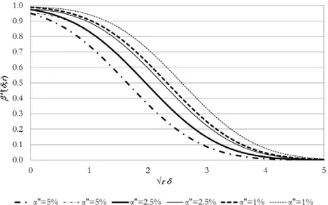
To complete the analysis of the second test, the Figure 2 represents the operative characteristic function of the conditioned test

_{β δ}

''

( )

_;

r

_{expressed in terms of}

_r

_δ

_{for the unilateral test in}

we have considered the values

_α

''

₌

_{1%, 2.5%, 5%}

_{. We note that in the graph the thick lines}

are referred to unilateral test, while the fine lines are referred to the bilateral test.

Figure 2 – Characteristic function of the conditioned test β δ''

( )

; . r

The figure shows the influence of the values

α

'' on the operative characteristic function. In particular the higher is the value of

α

'' than

β δ

''

( )

;

r

is much more sensitive. Moreover for the unilateral test the curves drawn on the graph identify the single values of the characteristic function. Instead, for the bilateral test instead you get a range of values for this function making able, as shown in the table above, the bilateral test to be perfectly symmetric or to be reduced to the unilateral case.

For the joint test of hypothesis, Table 3 contains the global significance level

α

given by equations (11) and (13) for the non-randomized test and randomized test respectively with respect to the conditions of the null hypothesis of the first and the second test together. We remember that in this case, for

∆ =

0

and

δ

=

0

we have

α α α

≤

'

+

'' and the equality is valid only in the situation of stochastic independence of the two systems of hypotheses. In the table the probability

α

is here obtained as function of

n

=

100, 250, 500

;

p

₀

=

0.01, 0.05, 0.10

and ' ''

_{2.5%, 5%}

TABLE 3 Global significance level α.

n p0 λ0 g(0; )λ0 ' '' _2.5% α =α = α'=α''=5% non-randomized test randomized

test randomized test non- random-ized test

0.01 1 0.3679 3.43 4.02 4.96 7.91 100 0.05 5 0.0067 3.82 4.92 7.99 9.72 0.10 10 ~ 0 3.89 4.94 9.63 9.75 0.01 2.5 0.0821 3.68 4.73 8.58 9.34 250 0.05 12.5 ~ 0 4.19 4.94 7.91 9.75 0.10 25 ~ 0 4.69 4.94 9.73 9.75 0.01 5 0.0067 3.82 4.92 7.99 9.72 500 0.05 25 ~ 0 4.69 4.94 9.73 9.75 0.10 50 ~ 0 4.8 4.94 9.03 9.75

Global significance level in the situation of stochastic independ-ence of the two systems of

hy-potheses

4.94 9.75

From Table 3 we observe that smaller is the sample size n much more visible are the differences of the probability values

α

obtained with randomized and non-randomized procedures. The last line in the table contains the global significance level in the situation of stochastic independence of the two systems of hypotheses. This situation is verified only when the probability that there are no accounting errors is

g

(

0;

λ

₀

)

~ 0

. In these cases we note that the probability obtained with the randomized test is exactly that of the situation of independence. For the situations where

g

(

0;

λ

₀

)

>

0

the differences are due to the fact that the second test is conditioned to the result of the first one.

To evaluate the sensitivity of the parameters

∆

and

δ

on the operational characteristic function

β

(

∆

;

δ

)

, we present in the next figures the level curves (

β

probabilities) for

β

=

20%, 40%, 60%, 80%

for the unilateral test to vary of

∆

and

δ

. We remember that as indicated in paragraph 3.2, the level curves for the unilateral test express also the extreme situation for the bilateral test. The considered cases are for

α α

'

=

''

=

2.5%

;

n

=

100, 250

and

p

₀

=

0.01, 0.05, 0.10

.

In particular, for

n 100

=

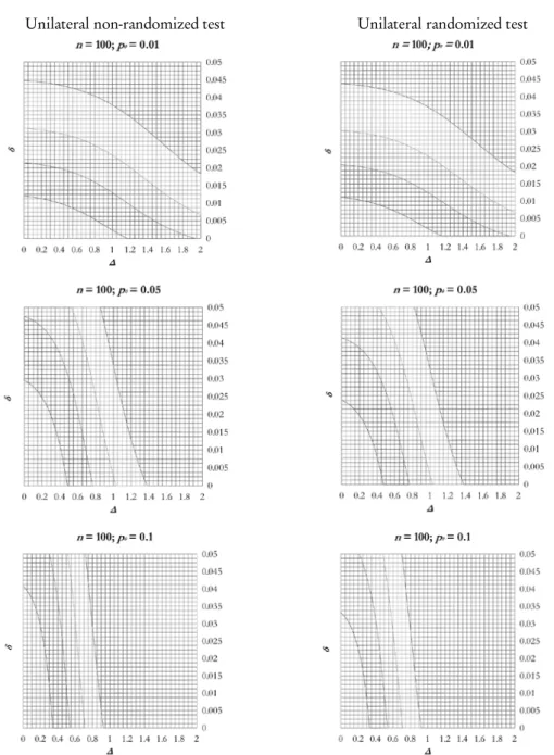
we have the following level curves for the non-randomized and for the randomized test.

Unilateral non-randomized test Unilateral randomized test

Figure 3 – Level curves for the unilateral non-randomized and randomized test for α α'= ''= 2.5%;

n 100= and p0=0.01, 0.05, 0.10.

For

n 250

=

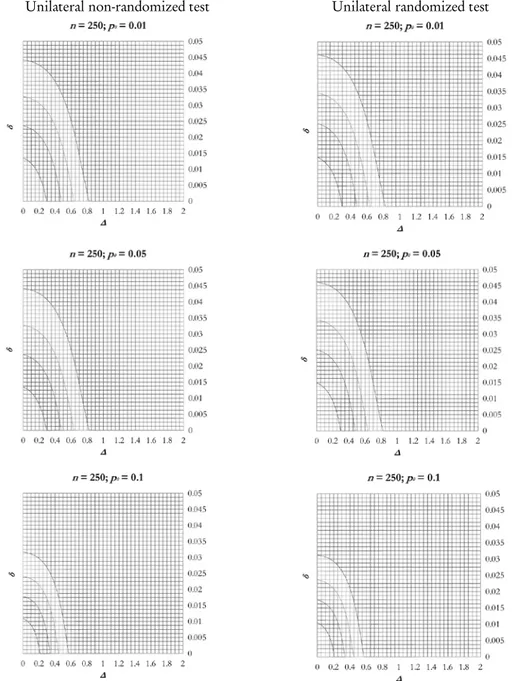
we have the following level curves for the non-randomized and for the randomized test.

Unilateral non-randomized test Unilateral randomized test

Figure 4 – Level curves for the unilateral non-randomized and randomized test for α α'= ''= 2.5%;

n 250= and p₀=0.01, 0.05, 0.10.

Observing the figures 3 and 4 we note that there is not a great difference in the level curves between non-randomized and randomized tests, for a fixed value of the sample size

n

. While in those figures we observe some differences of the level curves when

p

₀ varies, for a fixed

n

, or

The following table shows the values of

β

(

∆

;

δ

)

for a particular couple of

∆

and

δ

. In particular here we have considered

∆ =

0.01

and

δ

=

0.5

for

α α

'

=

''

=

2.5%, 5%

.

TABLE 4

Global Percentage values of β

(

∆;δ

)

for ∆ =0.01 andδ = 0.5 .

n p0 λ0 g(0; )λ0 ' '' _2.5% α α= = _{α α}'₌ ''_=5% unilateral non- random-ized test unilateral random-ized test bilateral non- random-ized test bilateral random-ized test unilateral non- random-ized test unilateral random-ized test bilateral non- random-ized test bilateral random-ized test 0 1 0.3679 78.44 76.91 81.25 79.63 73.65 66.51 78.11 70.25 100 0.1 5 0.0067 74.45 72.79 81.38 79.46 62.59 60.67 71.67 69.33 0.1 10 ~ 0 60.89 59.97 70.34 69.2 47.14 47.07 58 57.9 0 2.5 0.0821 63.32 58.95 67.87 63.07 46.84 45.37 51.95 50.27 250 0.1 12.5 ~ 0 47.08 47.77 58.51 57.29 36.38 34.87 47.07 44.97 0.1 25 ~ 0 25.53 25.43 34.67 34.53 16.36 16.36 24.54 24.53 0 5 0.0067 41.54 36.49 46.58 40.76 28.33 24.83 33.41 29.17 500 0.1 25 ~ 0 20.84 20.68 28.81 28.57 12.58 12.58 19.22 19.21 0.1 50 ~ 0 4.42 4.41 7.56 7.54 2.2 2.18 4.31 4.26

The table confirms as observed in the previous figures that there are modest differences between randomized and non-randomized test. These differences are greater for

p

₀

=

0.01

. The differences between unilateral and bilateral tests are quite reduced, too. The analysis confirms that the influence on the level curves is given mainly by

n

.

5.

FUTURE DEVELOPEMENTS

It is of fundamental importance to adapt the decision making of corporate management to changing conditions due to vary the change of the behaviour of customers, suppliers and the production system itself, for the employment of innovative technological tools and communication instruments, that compel to follow the multiple transactions that the company carries out. Therefore the statistical tools are increasingly made suitable for a dynamic vision.

The proposed procedure provides a tool of quantitative measure in terms of probability error that detects the anomalous circumstances in the accountancy book. The choice of values and parameters has an impact on the economic consequences and on the efficiency of the auditing, but also provides to the statistical analyst an easy to implement and to use procedure. In particular, it is of great importance the choice of the starting parameters

p

₀,

µ

₀,

n

and of the probabilities

α

' and

α

'' to evaluate the parameters influence on the selective ability

β

of the test. Therefore it should be interesting to conduct in the future a more analitical study concerning the selection of these parameters.

Moreover in this analysis we have made some assumptions regarding the distribution laws of some random variables. In particular in the first hypothesis system we have supposed that the

number

r

of units characterised by a book error in the sample is distributed as a Poisson random variable (considered acceptable the conditions of the asymptotic approximation of hypergeometric and binomial distribution to the Poisson distribution). While in the second hypothesis system we have assumed that the sample mean follows a normal distribution. Given the validity of these assumptions in standard situations, it should be interesting carry out further analysis to assess the changes in the sensitivity of the procedure. In particular, it should be interesting to consider some distributions for the error random variable

X

different from normal distribution, for example lognormal, chi-square and Weibull distributions.

In addiction as location index it is possible to use the median (or another quantile point) as an alternative to the mean so it should be possible to use a non-parametric version of the procedure.

Finally, a further consideration reguards the type of sampling carried out. In the present work we have considered a simple random sample, but it should be interesting to see how the procedure changes by performing a sampling whithout replacement.

ACKNOWLEDGEMENTS

The authors gratefully acknowledge Professor U. Magagnoli for his suggestions and supervision on the paper.

REFERENCES

A.A.ARENS,J.K.LOEBBECKE (2002). Applications of Statistical Sampling in Auditing. Englewood

Cliffs, Prentice Hall.

A.H. ASHTON, R.H. ASHTON (1988). Sequential Belief Revision in Auditing. The Accounting

Review, Vol. LXIII, 4, 623-641. AU Section 350. Audit Sampling. AICPA.

http://www.aicpa.org/Research/Standards/AuditAttest/DownloadableDocuments/AU-00350.pdf.

Retrieved 1 December 2012.

R.J.BOLTON,D.J.HAND (2002).Statistical Fraud Detection: A Review. Statistical Science, Vol. 17,

3, 235-255.

L.D.BROWN,M.S.ROZEFF (1979). Univariate Time-Series Models of Quarterly Accounting Earnings

per Share: A Proposed Model. Journal of Accounting Research, Vol. 1, 17, 179-189.

G.CAPRARA (1988). Stato e prospettive dell’impiego della statistica e dell’informatica nella moderna

gestione aziendale: il problema della formazione professionale. Statistica, Vol. XLVIII, 649-665. P.M.CHIODINI,U.MAGAGNOLI (2004). L’impiego dei metodi statistici nel controllo dinamico della

gestione aziendale. Relation presented to the Conference MTISD “Metodi, Modelli e Tecnologie dell’Informazione a Supporto delle Decisioni”, Università del Sannio, Benevento, 24-26 June 2004, 1-4.

R.CLEARY,J.C.THIBODEAU (2005). Applying Digital Analysis Using Benford’s law to detect Fraud:

D.M.GUY,D.R.CARMICHAEL,R.WHITTINGTON,(2002). Audit Sampling: an introduction. John

Wiley & Sons, New York.

R.W.HOUSTON,M.F.PETERS,J.H.PRATT (1999).The Audit Risk Model, Business Risk and

Audit-Planning Decisions.The Accounting Review, Vol. 74, 3, 281-298.

G.K. KANJI (2004). Total Quality Management and Statistical Understanding. Total Quality

Management, 5, 105-114.

J.KRIENS,R.H. VEENSTRA (1985). Statistical Sampling in Internal Control by Using the

AOQL-System. The Statistician, 34, 383-390.

R.LIBBY,J.T.ARTMAN,J.J.WILLINGHAM (1985).Process Susceptibility, Control Risk, and Audit-Planning.The Accounting Review, Vol. 60, 4, 212-230.

K.-Y. Low (2004). The effects of Industry Specialization on Audit Risk Assessment and Audit-Planning Decisions. The Accounting Review, Vol. 79, 1, 201-219.

D.C.MONTGOMERY (2005). Introduction to Statistical Quality Control, 5th Edition. John Wiley &

Sons, New York.

T.M.F.SMITH (1976). Statistical Sampling for Accountants. Haymarket, London.

A.D. TEITLEBAUM, C.F. ROBINSON (1975). The Real Risks in Audit Sampling. Journal of

Accounting Research, 13, Studies on Statistical Methodology in Auditing, 70-91. SUMMARY

On a Test of Hypothesis to Verify the Operating Risk Due to Accountancy Errors

According to the Statement on Auditing Standards (SAS) No. 39 (AU 350.01), audit sampling is defined as “the application of an audit procedure to less than 100 % of the items within an account balance or class of transactions for the purpose of evaluating some characteristic of the balance or class”. The audit system develops in different steps: some are not susceptible to sampling procedures, while others may be held using sampling techniques. The auditor may also be interested in two types of accounting error: the number of incorrect records in the sample that overcome a given threshold (natural error rate), which may be indicative of possible fraud, and the mean amount of monetary errors found in incorrect records. The aim of this study is to monitor jointly both types of errors through an appropriate system of hypotheses, with particular attention to the second type error that indicates the risk of non-reporting errors overcoming the upper precision limits.