A STUDY ON THE SELECTION PATTERN OF PLAYERS IN
ANY TEAM SPORT
Moumita Chatterjee1
Department of Mathematics and Statistics, Aliah University, Kolkata, India
Sugata Sen Roy
Department of Statistics, University of Calcutta, Kolkata, India
1. INTRODUCTION
In recent times, statistical methods have been extensively used to analyze and assess sports data for developmental and tactical planning. Kimber and Hansford (1993) used a nonparametric method for assessing a player’s performance in cricket, where they in-troduced an alternative batting average method. Corralet al. (2008), while analyzing the pattern of player substitution during soccer matches, used an inverse Gaussian hazard model to reveal some interesting trends in substitution of players, especially with regard to home teams. Fricket al. (2009) analyzed the survival time of head coaches over a substantially longer period for first division German professional soccer, using the Cox PH model, the gap time method and some parametric methods like exponential and Weibull models. Oberhoferet al. (2015) discussed the similarities between the relega-tion and promorelega-tion system in European football with the exits and entries of firms in the usual goods and services market. Kachoyan and West (2018) derived an exact survival function for cricket scores and compared it with the existing product limit estimators of survival functions.
In the modern world, careers in every profession are becoming more and more com-petitive. Team sport is no exception. Players need to constantly perform in order to re-tain their places in the team. In team games, all members need to act cohesively in order to achieve their common goal. And each member needs to fulfill his designated role to ensure perfect balance. Hence the composition of the team depends on the individual performance of a player in his given role.
Usually, in the early stages of his career, a player is judged by his match to match performance. Once he proves his importance in the team, his place is cemented. But with time, the wear and tear of his physique takes its toll and makes him vulnerable to
446
injury and hence exclusion. In this paper, our objective is to capture these patterns of inclusion and exclusion of the players. The technique we apply can be extended to any team sport. However, our focus in this paper is to analyse the pattern of inclusion and exclusion of players in the ODI cricket teams of different countries.
Cricket ODI is a game played between two teams representing their respective na-tions and comprising of 11 players each. Both teams play an inning of 50 overs of 6 balls each. During an inning, the 11 players of one team goes out to field, while the opposi-tion batting team sends out 2 players to bat. The task of the two batsmen is to defend the two wickets fixed on either side of a 22 yard strip. The fielding side designates a bowler to bowl an over from one side of the pitch to the wicket on the other side. The bowler can bowl at most 12 overs but none consecutively. The batsman on the opposite side (the striker) both defends his wicket from being hit by the ball and also tries to score runs by hitting the ball and exchanging places with the other batsman across the pitch or by sending the ball beyond the boundary of the field. A bowler can get a batsmanout in several ways, including by hitting the wicket. After a batsman is out, a new batsman replaces him till either all 10 batsmen are out (leaving the last batsman with no partner) or the 50 overs are bowled. After both the teams have completed their innings, the team with the greater aggregate runs scored by their batsmen wins.
The data we use are on players who started their career after the International Cricket Council (ICC) World Cup in 2003. The study period ends in June, 2014. Since a mini-mum number of matches is required to ensure that there is enough scope for recurrences of both inclusion and exclusion, only those players who have played atleast 40 matches during this period are included in the study. The list contains male players from all the major cricket playing countries around the globe. This includes India, Australia, New Zealand, Sri Lanka, Pakistan, West Indies, South Africa and England, which are the top 8 cricket playing countries according to the ICC list. The list of players has 33 batsmen and 31 bowlers. Since the physical stress and the energy required of a bowler is usually greater than that of a batsman, they are also more injury-prone. Added to this is the fact that the selection of a bowler depends more on the weather and pitch conditions. Hence it is likely that the batsmen and bowlers would show substantially different survival pat-terns. Hence we have segregated the players into two strata, one comprising batsmen and the other comprising bowlers. The inclusion and exclusion patterns are studied for each stratum assuming interdependence both between the selections and non-selections as also between successive selections and non-selections.
There have been plenty of articles based on recurrent events. Reviews of early studies in this area can be found in Kalbfleisch and Prentice (1980) and Clayton (1994). Several authors, Twisket al. (2005); Thomsen and Parner (2006); Liu et al. (2004) have used longi-tudinal health care data to study recurrent events. Applications of the methods in social sciences can be found in Ham and Rea (1987) and Chan and Stevens (2001), where pat-terns of the recurrence of unemployment are looked into. The term "recurrent episode" data has been coined by Hougaard (2000), who presents a detailed discussion of handling such data. However, there has been very few studies on alternating recurrent events. Gap time methods have been applied by Linet al. (1999); Wang and Chang (1999); Pena
et al. (2001), while Yan and Fine (2008) used temporal process regression to analyse re-current episode data in cystic fibrosis patients. Sen Roy and Chatterjee (2015) analysed data of this kind without considering the correlation between the alternating events. A copula based approach which accounted for the correlation between the alternating events was used by Chatterjee and Sen Roy (2018a) to study the time to infection and time to cure of the cystic fibrosis data.
In this paper we apply techniques similar to Chatterjee and Sen Roy (2018a) to study the cricket data. However, the focus here is more on the identification of patterns in cricket players’ inclusion in or exclusion from their teams, rather than on theoretical developments. To do this we first needed to identify the underlying distributions and then to test whether the separation of the players into two strata is justified. The sur-vival functions are then obtained taking into account the dependence between cycles. In Section 2 we describe the model. The main section is the third, which shows the detailed analysis of the ODI cricket data. Finally, some concluding remarks are made in Section 4.
2. THE MODEL
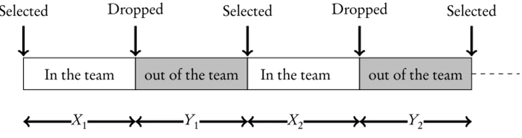
Let the two events be theselection of a player in the team for a match and the dropping of a player from the team for a match. The selection for a match is followed by the cycle inclusion when the player retains his place in successive matches. This ends with the event dropped, after which the player is in the cycleexclusion, where he sits out succes-sive matches till the event selection happens again. The two cycles are thus alternating recurrent. Figure 1, gives a graphic idea of this recurrences.
In the team out of the team In the team out of the team
X1 Y1 X2 Y2
Selected Dropped Selected Dropped Selected
Figure 1 – Showing recurrences of inclusion and exclusion for a particular individual.
LetX and Y denote respectively the lengths of inclusion and exclusion as measured by the number of consecutive matches played and the number of consecutive matches sat out by a player. A complete cycle is then composed of two alternating cycles of inclusion and exclusion, withXj+ Yj the length of thejthcycle. Letn be the number of individuals in the study. For theith individual in the study, letm
i be the number
448
X1i,· · · , Xmii ofinclusion-times each culminating in the event dropped and a sequence
Y1i,· · · , Ymii ofexclusion-times each culminating in the event selected. (Xj i,Yj i) then gives the complete cycle for the jth recurrence of inclusion and exclusion for the ith individual with cycle lengthXj i+ Yj i.
To study the patterns in these inclusion and exclusion cycles, we adopt a modified version of the technique used by Chatterjee and Sen Roy (2018a).
Assume thatXj andYj follow the distribution functions FX
j(x,θj) and FYj(y,ηj)
respectively, whereθj = (θ1j, . . . ,θp j)0 andη
j = (η1j, . . . ,ηq j)0 are respectively the p andq dimensional parameter vectors characterizing the two distributions. Since Xjand Yj are likely to be dependent, we need to consider the joint distribution of(Xj,Yj). Since the joint distribution of positive random variables are generally not of a closed form, we use a copula function to obtain the joint distribution function as
FX
jYj(x, y,ζj) = C (FXj(x,θj), FYj(y,ηj),ξj), (1)
whereζj= (θj0,ηj0,ξ
j)0andξjis a dependence parameter indicating the strength of the relationship betweenXj iandYj i.
Since in our data, all players are observed only from their ODI debut, it is obvious thatXj i precedesYj i, for alli = 1,..., n. The survival and hazard functions of Xj i can thus be obtained directly from the marginal distribution function as
SX j(xj i,θj) = 1 − FXj(xj i,θj) (2) and λX j(xj i,θj) = − d d xj il nSXj(xj i,θj), (3)
respectively. However, the survival and hazard functions forYj i are conditioned on Xj i= xj i. Since the conditional distribution ofYj i|Xj i= xj i is
FY j|Xj(yj i,ζj|xj i) = CX0 (FX j(xj i,θj), FYj(yj i,ηj),ξj) fX j(xj i,θj) , (4)
these are given respectively by SY
j|Xj(yj i,ζj|xj i) = 1 − FYj|Xj(yj i,ζj|xj i) (5)
and λYj|Xj(yj i,ζj|xj i) = −
d
d yj il nSYj|Xj(yj i,ζj|xj i). (6)
Having accounted for the dependence between inclusion and exclusion times, we next model the dependence over the cycles. This is necessary as it is likely that theXj i’s would increase with j as a player establishes himself in the team. Of course, injury and
other such factors may induce a decline in the latter cycles of a player’s career. On the other hand,Yj i’s are likely to decrease with j , with possibly moderate increases due to longer recuperation periods at the latter cycles. However, whatever be their form, it is clear that there is a relationship between successiveXj i’s andYj i’s.
Since the distributional parameters characterize the event times, an way to accom-modate this dependence would be through the distribution parameters. To accommo-date the relationships between theXj i’s, the parametersθj are linked throughθk j = gk(j,αk), k = 1,..., p and j = 1,..., mi, whereαk’s arerk-dimensional parameter vec-tors which characterize the functions gk fork = 1,..., p. Similarly, the relationships between theYj i’s are modelled through the parameters asηl j = hl(j,βl), l = 1,..., q and j = 1,..., mi, withβl’s thesl-dimensional parameter vectors characterizing the functionshl forl = 1,..., q. Like the θj i’s andηj i’s, the dependence parametersξj’s are related throughξj= u(j,κ), where κ = (κ1, . . . ,κd)0is the d-dimensional parameter vector characterizing the functionu. The gk,hlandu functions allow us to capture the pattern that the two events exhibit over the cycles.
However, before constructing the likelihood function we need to take account of possible censorings.This may happen owing to the termination of the study or because of a player retiring. Up till now, we have implicitly assumed that we observe the whole cycle (starting from a selection through an exclusion to a re-selection), i.e. a player is in the cycleexclusion and experiencing the event selection at the instant of the termination of the study. However a player may be in the cycleinclusion and experiencing the event dropped at the time of termination. In fact, an observation need not end with any event and a player may voluntarily withdraw from the study due to retirement or the player may be in the middle of a cycle at the time of the termination of the study. His obser-vation is then censored in that cycle. To incorporate these into our model we define for theithplayer the following indicator functions :
δ∗ j i= 1 for all j= 1,··· , mi− 1
1 if j= mi and theithindividual withdraws while sitting out or at the instance of selection
0 if j= mi and theithindividual withdraws while playing or at the instance of being dropped
δ1j i=
1 for all j= 1,··· , mi− 1
1 if j= mi and theithindividual is dropped
0 if j= mi and theithindividual withdraws while palying
δ2j i=
1 for all j= 1,··· , mi− 1
1 if j= mi and theithindividual is selected
450
δ∗
j iin conjunction withδ1j iandδ2j i indicate whether theithplayer exits while ex-periencing the eventselection or the event dropped or is censored while in cycle inclusion or in cycleexclusion.
The likelihood function can then be constructed as l(α, β, κ) = l(α,β,κ|(xj i,yj i), j = 1...,4, i = 1,... n) = Yn i=1 Y j=1,···,4 SX j(xj i,θj)¦λXj(xj i,θj ©δ1j i n SY j|Xj(yj i,θj,ηj)¦λYj|Xj(yj i,θj,ηj) ©δj ioδ ∗ 2j i . (7)
The maximum likelihood (m.l.) estimates(ˆα0, ˆβ0, ˆκ0) are then obtained by applying the Newton-Raphson method. This for any cycle j leads to the estimator(ˆθ0j, ˆη0j, ˆξ ) of the model parameters and hence to the estimators ˆSX
j(xj i, ˆθj) and ˆSYj|Xj(yj i, ˆθj, ˆηj,ξj|xj i)
of the respective survival functions and their corresponding hazard functions.
3. ANALYSIS OF THEODICRICKET DATA
3.1. Data
As mentioned in the introduction, we consider 64 cricketers, who have played a
min-imum of 40 matches. They are segregated into two strata, withbatsmen in Stratum 1
andbowlers in Stratum 2 with respective sizes n1= 33 and n2= 31 (we use superscripts 1 and 2 to identify the variables and parameters of the respective stratum). The data on these 64 players are obtained from the archives ofwww.espncricinfo.com. For each player we compute the lengths of consecutive matches played (X ) followed by the number of consecutive matches sat out (Y ). The two together gives us a complete cycle. As it is observed that data beyond the 4thcycle is sparse, we consider only 4 cycles and assume that beyond this the observation is censored i.e. we take max(mi) =4. Thus for each of the 64 players we have his 4 (or less) cycle lengths and his censoring indicator. The method, as described in Section 2, is then applied to each of the two strata separately.
3.2. Analysis
To begin with, we test whether our conjecture that the batsmen and bowlers exhibit dif-ferent survival patterns is correct or not. For this, letSX(k)
j(t) and S
(k)
Yj(t), j = 1,...4; k = 1, 2 denote the survival functions for the two events for different cycles for each of the
two strata. We then employ the Mantel-Haenszel statistic (Klein and Moeschberger, 2003) to test separately for j= 1,...4,
H0X j:SX(1) j(t) = S (2) Xj(t) against H1X j:S (1) Xj(t) 6= S (2) Xj(t) and H0Y j:SY(1) j(t) = S (2) Yj(t) against H1Y j:S (1) Yj(t) 6= S (2) Yj(t).
Table 1 shows thevalues corresponding to the tests. We find that most of the p-values are small. This indicates a significant difference between the survival functions of the two groups. Hence we feel justified in modelling the survival functions for the batsmen and bowlers separately.
TABLE 1
Results showing the p-values for testing the similarities in survival curves among batsmen and bowlers.
Cycle Number of matches played Number of matches sat out
1st 0.008 0.01
2nd 0.1 0.03
3rd 0.01 0.2
4th 0.06 0.09
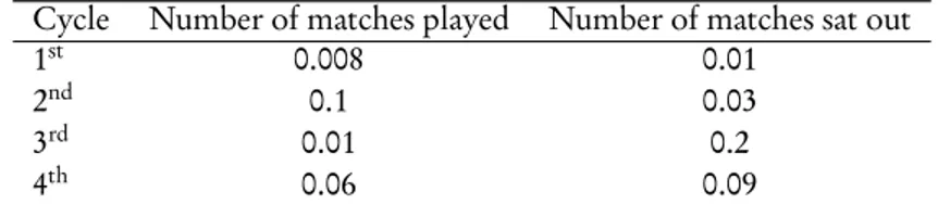
To choose the appropriate underlying distributionsFX(k)andFY(k)for thekthstratum, k = 1,2, we fit several alternative distributions to each of Xj(k)andYj(k)separately for each cycle within the stratum. Mainly the Log-normal, Weibull and Log-logistic distri-butions are considered. The survival curve for each of these distridistri-butions is compared with the empirical survival curve obtained by the Kaplan-Meier estimator. As an exam-ple, in Figure 2, we have plotted the survival curves for inclusion and exclusion in the 1st cycle for both strata. From the plot, it is discernible that the Weibull matches the KM curve most closely in each of the plots. In fact, the Weibull gives the best fit for both Xj(k)andYj(k)for most of the four cycles fork= 1,2.
However, to substantiate the result, we use the following method. For each of the plots, we first select a number of time points. Then for each of the log-normal, Weibull and log-logistics curves, the sum of squared difference (SSD) between the survival prob-abilities at these points with that on the KM curve is obtained. The curve with the minimum SSD is then chosen. These results, as shown in Table 2, also indicate that the Weibull gives the best fit for most of the cycles for both the strata.
As reasoned later, for uniformity, we discard the occasional non-Weibull best-fit dis-tributions, and select the Weibull as the underlying distribution for all j= 1,...4; k = 1, 2 for both inclusion and exclusion.
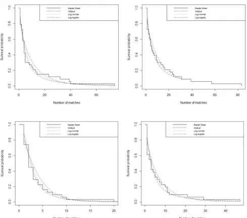
Next, in Figure 3 we plot the four Weibull curves for the four cycles in the same graph for each of the two events in the two strata. There is some indication that some
452
Figure 2 – Plots for the 1stcycle comparing the fitted log-normal, Weibull and log-logistic curves
with the Kaplan Meier curve (in the order batsmen inclusion and exclusion and bowler inclusion and exclusion, clockwise from upper left).
T ABLE 2 R esults sho wing the SSD’ s for the dif fer ent distr ibutions. N umber of matc hes pla y ed until dr opped N umber of matc hes sat out Cy cle W eibull Log-nor mal Log-logis tic W eibull Log-nor mal Log-logis tic Batsman Bo w ler Batsman Bo w ler Batsman Bo w ler Batsman Bo w ler Batsman Bo w ler Batsman Bo w ler 1 st 0.049 0.052 0.07 0.069 0.119 0.096 0.046 0.067 0.051 0.081 0.076 0.101 2 nd 0.111 0.062 0.191 0.103 0.198 0.115 0.129 0.16 0.100 0.117 0.119 0.157 3 rd 0.149 0.13 0.227 0.143 0.25 0.17 0.162 0.21 0.18 0.284 0.204 0.295 4 th 0.226 0.182 0.310 0.217 0.383 0.249 0.241 0.35 0.201 0.29 0.251 0.301
454
Figure 3 – Plots for the 1stcycle comparing the fitted log-normal, Weibull and log-logistic curves
with the Kaplan Meier curve (in the order batsmen inclusion and exclusion and bowler inclusion and exclusion, clockwise from upper left).
pattern in this, although there are quite a few anomalies as well. For example, in case of inclusion, both strata show an ordering in the first, third and fourth cycles (with the curves progressively lying above the lower cycle curves). However, the second cycle curve lies lower than the other three for batsmen, but only lower than the fourth for bowlers. Since careers in sports do not exhibit such random patterns, we decided to incorporate some dependence structure over the cycles.
As has been discussed in Section 2, to take care of the dependence we need to string the parameters through the functions g and h. In fact, for this reason we had ignored the occasional non-Weibull best-fit distributions and assumed the Weibull distribution uniformly for all cycles both over the two events and the two strata.
Assume thatXj(k)∼ W (θ1(k)j,θ(k)2j) and Yj(k)∼ W (η(k)1j,η(k)2j) for j = 1,2,3,4 and k = 1, 2. Hereθk
1jandηk1jare the scale parameters andθk2jandη2kjare the shape parameters of the respective distributions.
Next we plot(j,θ(k)l j ) and (j,η(k)l j) for each l = 1,2 and k = 1,2. Unfortunately, since we have only 4 cycles, only a rough idea of the functional forms can be derived from these. The plots indicate that the logarithm of the distributional parameters are linear in the order of the cycle. Moreover, the distributional parameters are all non negative. Hence we assume the following relationships: for the batsmen, the parameters are related as θ(1)1j = eα(1)11+α (1) 12j and θ(1) 2j = e α(1) 21+α (1) 22j; η(1)1j = eβ(1)11+β (1) 12j and η(1) 2j = e β(1) 21+β (1) 22j; j= 1,··· ,4,
while for the bowlers the relationships are
θ(2)1j = eα(2) 11+α (2) 12j and θ(2) 2j = eα (2) 21+α (2) 22j; η(2)1j = eβ(2) 11+β (2) 12j and η(2) 2j = eβ (2) 21+β (2) 22j; j= 1,··· ,4.
Having decided on the marginal distributions and the functional relationships be-tween the parameters, we formulate the joint distribution of(Xj(k),Yj(k)) through a cop-ula. For this we use the Clayton copula which is widely accepted as the most suited for bivariate Weibull distributions. The dependence parameterξj(k) involved in the cop-ula is estimated for each j by using it’s relation with Kendall’sτ. The ξj(k)values for the two strata come out to be approximately constant, withξj(1)≈ −0.3 for Stratum 1 and
ξj(2)≈ −0.05 for Stratum 2. Hence it is not required to determine the functional form for stringing the dependence parameter.
The likelihood function (7) is then built on the basis of the survival and hazard func-tions (2) - (6) and the parameters (αk
456
andk= 1,2 are estimated using the Newton-Raphson method. The estimated θk
l j and
ηk
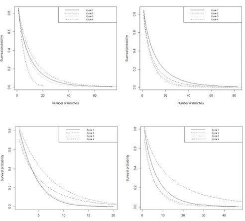
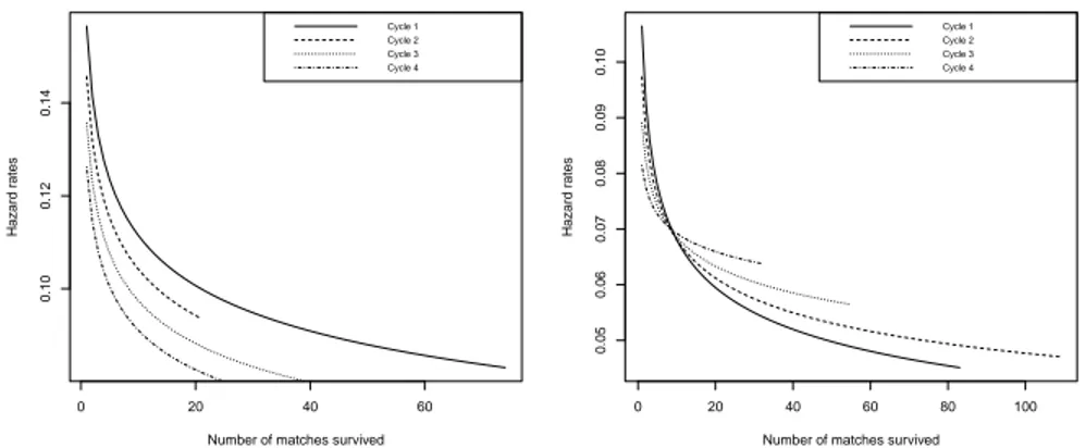
l j,k= 1,2; l = 1,2; j = 1,2,3,4 are then obtained by using the respective relationships. These are shown in Table 3. The hazard curves for the batsmen and bowlers for both inclusion and exclusion are shown in Figures 4 and 5, respectively.
4. RESULTS AND DISCUSSION
4.1. Batsmen
Table 3 shows that the estimated shape parameters ˆθ(1)2j and ˆη(1)2j are all less than one. This implies that the failure rates are all decreasing with the number of matches played. Figure 4 indicates that, for the batsmen, the hazard of being dropped is greater in the initial cycles than in the later cycles. This clearly suggests that at the beginning of their career, a batsman is quickly dropped if he does not perform. However, once a batsman has been in the team for a long period and has played a large number of matches, his chances of playing are much greater as compared to a newcomer. This is similar to the concept ofwork hardening in reliability theory. Moreover, the hazard rates fall off very rapidly, which implies that a batsman, once selected, is not easily dropped. On the other hand, as the right panel shows, the hazard for selection has an insignificant difference over the cycles. Interestingly, these hazard curves intersect. They are flatter for latter cycles than for early cycles. This means that although when a batsman is dropped from the team his experience gives him only a slight advantage in terms of a recall, the chances of recall for a senior player remains relatively constant with the number of matches sat out, while the chances of recall for a newcomer falls off more rapidly with the number of matches he misses.
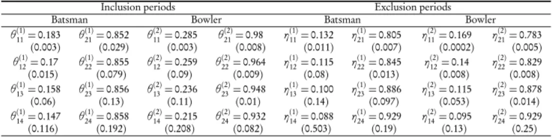
TABLE 3
Showing the estimatedθ(k)l j andη(k)l j,k= 1,2; l = 1,2; j = 1,2,3,4.
Inclusion periods Exclusion periods
Batsman Bowler Batsman Bowler
θ11(1)= 0.183 θ (1) 21= 0.852 θ (2) 11= 0.285 θ (2) 21= 0.98 η (1) 11= 0.132 η (1) 21= 0.805 η (2) 11= 0.169 η (2) 21= 0.783 (0.003) (0.029) (0.003) (0.008) (0.011) (0.007) (0.0002) (0.005) θ(1) 12= 0.17 θ(1)22= 0.855 θ(2)12= 0.259 θ(2)22= 0.964 η(1)12= 0.115 η(1)22= 0.845 η(2)12= 0.14 η(2)22= 0.829 (0.015) (0.079) (0.09) (0.009) (0.08) (0.013) (0.008) (0.008) θ(1) 13= 0.158 θ(1)23= 0.856 θ(2)13= 0.236 θ(2)23= 0.948 η(1)13= 0.100 η(1)23= 0.886 η(2)13= 0.115 η(2)23= 0.878 (0.06) (0.13) (0.11) (0.01) (0.14) (0.097) (0.053) (0.014) θ(1) 14= 0.147 θ(1)24= 0.858 θ(2)14= 0.215 θ(2)24= 0.932 η(1)14= 0.088 η(1)24= 0.929 η(2)14= 0.095 η(2)24= 0.929 (0.116) (0.192) (0.208) (0.082) (0.503) (0.19) (0.13) (0.25)
0 20 40 60
0.10
0.12
0.14
Number of matches survived
Hazard r ates Cycle 1 Cycle 2 Cycle 3 Cycle 4 0 20 40 60 80 100 0.05 0.06 0.07 0.08 0.09 0.10
Number of matches survived
Hazard r ates Cycle 1 Cycle 2 Cycle 3 Cycle 4
Figure 4 – Batsmans’ hazard curves for the events dropped (left panel) and selected (right panel).
0 10 20 30 40 0.16 0.18 0.20 0.22 0.24 0.26 0.28
Number of matches survived
Hazard r ates Cycle 1 Cycle 2 Cycle 3 Cycle 4 0 50 100 150 0.06 0.08 0.10 0.12
Number of matches survived
Hazard r ates Cycle 1 Cycle 2 Cycle 3 Cycle 4
458
4.2. Bowlers
The pattern for bowlers is somewhat different. As Table 3 shows, the estimated shape parameters ˆθ(2)2j and ˆη(2)2j are again all less than unity, and hence the failure rates are all decreasing with the number of matches played. However, Figure 5 shows that in this case, the difference between the hazard curves of the four cycles are much less. This im-plies that very little distinction is made between continuity and change in terms of both selection and exclusion. Further, the hazard curves are flatter, implying that the chances of being dropped or selected does not change too rapidly with the number of matches played or sat out. These are unlike what we observe for the batsmen and may perhaps be because bowlers are primarily selected on the basis of the pitch-conditions and hence have less secure places in the team, irrespective of their length of inclusion. Because of the more physical nature of their job, fatigue or injury too may be important factors. However, here too the hazard rates are low implying that once selected or dropped, the chances of a reversal is low.
5. CONCLUDING REMARKS
In general, our study shows that the position of a batsman is more stable in a team, par-ticularly once he has established himself after the first few cycles. But once dropped, it is more difficult for him to make a comeback. For the bowlers, the more physical nature of their job, makes for greater rotation of their places in the team, so that they are more likely to be quickly dropped and also quickly selected than batsmen. In fact, since bowlers can be vastly different in their trade, their selection depends on a host of other factors like the pitch condition, weather condition or even the proclivity of the opposition batsmen. Hence their survival patterns are distinctly different.
The selection of players, particularly bowlers, depend, besides their abilities, on a host of other factors. Having established that there are distinct patterns in their selec-tion, in future studies we hope to find more specific reasons behind these patterns using appropriate covariates as in Chatterjee and Sen Roy (2018b). However, many of these factors, like pitch condition, type of opposition, etc., are somewhat subjective in nature and hence data on these are difficult to find and even more difficult to quantify. Once the relevant covariates are identified and the measurement issues resolved, regression-type survival models can be used to identify the factors behind the inclusion and exclusion patterns of players.
REFERENCES
S. CHAN, A. STEVENS(2001).Job loss and employment patterns of older workers. Journal of Labor Economics, 19, no. 2, pp. 484–521.
functions of two alternating recurrent events. Journal of Statistical Computation and Simulation, 88, no. 16, pp. 3098–3115.
M. CHATTERJEE, S. SENROY(2018b).Estimating the hazard functions of two
alternat-ing recurrent events in the presence of covariates. AStA Advances in Statistical Analysis, 102, no. 2, pp. 289–304.
D. CLAYTON(1994). Some approaches to the analysis of recurrent event data. Statistical
Methods in Medical Research, 3, no. 3, pp. 244–262.
J. D. CORRAL, C. BARROS, J. PRIETO-RODRIGUEZ(2008). The determinants of soccer
player substitutions: A survival analysis of the Spanish soccer league. Journal of Sports Economics, 9, no. 2, pp. 160–172.
B. FRICK, C. BARROS, J. PASSOS(2009).Coaching for survival: The hazards of head coach careers in the German Bundesliga. Applied Economics, 41, no. 25, pp. 3303–3311.
J. HAM, S. REA(1987). Unemployment insurance and male unemployment duration in
Canada. Journal of Labor Economics, 5, no. 3, pp. 325–353.
P. HOUGAARD(2000). Analysis of Multivariate Survival Data. Springer-Verlag, New
York, 1st ed.
B. KACHOYAN, M. WEST(2018). Deriving an exact batting survival function in cricket.
In R. STEFANI, A. BEDFORD (eds.), 14th Australasian Conference on Mathematics
and Computers in Sport (ANZIAM MathSport 2018). University of Sunshine Coast, ANZIAM Mathsport, pp. 160–172.
J. D. KALBFLEISCH, R. L. PRENTICE(1980). The Statistical Analysis of Failure Time Data. John Wiley, New Jersey, 2nd ed.
A. KIMBER, A. HANSFORD(1993).A statistical analysis of batting in cricket. Journal of
the Royal Statistical Society, Series A, 156, pp. 443–455.
J. KLEIN, M. MOESCHBERGER(2003). Survival Analysis: Techniques for Censored and
Truncated Data. Springer, New York, 2nd ed.
D. LIN, W. SUN, Z. YING(1999).Nonparametric estimation of gap time distributions for serial events with censored data. Biometrika, 86, pp. 59–70.
L. LIU, R. WOLFE, X. HUANG(2004). Shared frailty models for recurrent events and a terminal event. Biometrics, 60, pp. 747–756.
H. OBERHOFER, T. PHILIPPOVICH, H. WINNER(2015).Firm survival in professional
sports: Evidence from the German football league. Journal of Sports Economics, 16, no. 1, pp. 59–85.
460
E. PENA, R. STRAWDERMAN, M. HOLLANDER(2001).Nonparametric estimation with
recurrent event data. Journal of American Statistical Association, 96, pp. 1299–1315. S. SENROY, M. CHATTERJEE(2015).Estimating the hazard functions of two alternately
occurring recurrent events. Journal of Applied Statistics, 42, no. 7, pp. 1547–1555.
J. THOMSEN, E. PARNER(2006). Methods for analysing recurrent events in health care
data: Examples from admissions in Ebeltoft health promotion project. Family Practice, 23, pp. 407–413.
J. TWISK, N. SMIDT, W. VENTE(2005).Applied analysis of recurrent events: A practical
overview. Journal of Epidemiology and Community Health, 59, pp. 706–710. M. WANG, S. CHANG(1999).Nonparametric estimation of a recurrent survival function.
Journal of American Statistical Association, 94, pp. 146–153.
J. YAN, J. FINE(2008).Analysis of episodic data with application to recurrent pulmonary exacerbations in cystic fibrosis patients. Journal of American Statistical Association, 103, pp. 498–510.
SUMMARY
In this paper, we study the pattern of inclusion and exclusion of players from a team in any team sport. Usually these inclusions and exclusions are related to the player’s performance in the matches previously played. Also the inclusion and exclusion at any particular cycle depends on the player’s history as observed through the number of times he has been included or excluded previously. The focus of this paper is to study this pattern for cricketers who have represented their respective countries in One Day Internationals (ODIs). As observed in the study, there is a distinct difference in the inclusion and exclusion patterns of bowlers and batsmen, and hence the two groups have been studied separately. Respective survival functions over the cycles of inclu-sion and excluinclu-sion have been constructed for both groups. These reveal several interesting features regarding the chances of an ODI cricketer being retained or dropped from the team.