UNIVERSITÀ POLITECNICA DELLE MARCHE
Department of Agricultural, Food and Environmental Sciences (D3A)
Scientific field: AGR/14 - Pedology
Ph.D. in AGRICULTURAL, FOOD AND ENVIRONMENTAL SCIENCE
XV (15°) edition (2013-2016)
"CHANGES OCCURRING IN THE TOPSOIL AND IN RHIZOSPHERE
UNDER FAGUS SYLVATICA ALONG A SMALL
LATITUDINAL-ALTITUDINAL GRADIENT
"
PhD Student: Tutor:
Valeria Cardelli Prof. Giuseppe Corti
Co-tutor:
PhD Stefania Cocco
Summary
1 Introduction ... 1
1.1 The rhizosphere ... 1
1.1.1 Definition and general properties ... 1
1.1.2 Methods to study and sampling the rhizosphere ... 4
1.2 The topsoil: organic and organo-mineral horizons ... 5
1.2.1 Definition and general properties ... 5
1.3 Bibliography ... 8
2 Aims of the research ... 11
Paper I ... 12
Paper II ... 26
Paper III ... 38
Paper IV ... 72
1 Introduction
Soil is a complex system largely affected by climate (Aerts, 2006). Temperature is one of the climate’s attribute, and its changing is one of the drivers of the soil physical, chemical and biochemical properties and functionality (Allen et al., 2011). Most of the studies on climate effect has dealt with the aboveground vegetation, plant diversity, or soil biochemistry (Hunt and Wall, 2002), but an extensive comprehension of the effect on soil functionalities is still poor, even if some studies have demonstrated the relationship between soil properties and climate change drivers. In particular, climatic stress such as warming has effect on the rhizosphere soil and topsoil, their microbial communities, and nutrient functioning.
The doctoral project focused on the investigation of the temperature effect on soil properties and processes. The project followed two main lines: i) the investigation of mineral soil, specifically of the rhizosphere effect on chemical soil properties, and ii) chemical and biochemical properties of the topsoil, which is formed by the organic horizons (litter and humus) and the first organo-mineral horizon in a gradient of decomposition.
The work on the organic horizons fell in a collaboration with the tem of prof. David Weindorf at the Texas Tech University of Lubbock (Texas, USA), where I developed an analytical method to estimate total carbon and total nitrogen with proximal sensors (PXRF1 and VisNIR2) on organic soil materials. The use of these apparata has been already extensively documented for mineral soil horizons, but there was no information on their use on organic horizons.
1.1 The rhizosphere
1.1.1 Definition and general properties
The rhizosphere is the interface between plant roots and soil, where the interactions between abiotic and biotic factors create a zone distinct from the bulk soil, the soil not directly affected by living roots and microorganisms (Haynes, 1990; Philippot et al, 2013). Indeed, rhizosphere is the most important link between plants and soil, plays a central role in the maintenance of the soil-plant system and, in spite of the small volume that it occupies, it influences the biogeochemistry of natural and agricultural ecosystems (Gobran and Clegg, 1996; Gobran et al., 1998). The term rhizosphere is self-explanatory: rhizo comes from the Greek word "root" and sphere stands for the "environment" in which roots act (Gobran et al., 1998). The rhizosphere is usually subdivided into three ecological niches (Lynch, 1990):
1
Portable X-Ray Fluorescence 2
• endorhizosphere, the thin layer that spans from the roots surface to the near surface cells, which is colonized or can be potentially colonized by microbes;
• rhizoplane, the external plant surface, namely the two-dimensional interface between root and soil;
• ectorhizosphere, the soil layer surrounding roots and affected by the activity of roots themselves, and the harboring microorganisms. The thickness of this portion usually ranges from one to a few millimeters.
In general, the term "rhizosphere" is used to indicate the whole environment between ecto- and endorhizosphere.
Rhizosphere effect
Ectorhizosphere and rhizoplane represent the major source of substrates for microbial activity due to their enrichment with rhizodeposition products (Lynch and Whipps, 1990). Rhizodeposition is the release of carbon compounds from living plant roots through the loss of organics from root epidermal and cortical cells that leads to a proliferation of microorganisms in this soil portion. Also root metabolite and root exudates are often released in large quantities into the rhizosphere from living root hairs or fibrous root systems (Bertin et al., 2003). Theoretically, almost any soluble component present inside the root can be released to the rhizosphere; however, evidences suggest that exudation is dominated by low molecular weight solutes such as sugars, amino acids and organic acids that are present in the cytoplasm at high concentrations (Farrar et al., 2003). Through the exudation of this wide variety of compounds, roots impact the soil microbial community in their immediate vicinity, influence resistance to pests, support beneficial symbioses, alter the chemical and physical properties of the soil, and inhibit the growth of competing plant species (Bertin et al., 2003). However, their production is substantially dependent on the soil and other environmental conditions, such as anoxia, mechanical force, water stress, nutrient status, temperature, pH and day-length (Cheng et al., 1993).
Another important process occurring at high extent in this soil fraction, and that is able to increase C release, is respiration. Functionally, rhizosphere respiration consists of root respiration, together with microbial respiration due to the use of root-derived materials (rhizodeposition) by microbes. The ecological implications of root respiration are different from those of root exudation. Root respiration consists of a direct release of photosynthetically-fixed C, whereas root exudation is a process through which photosynthetically-fixed C enters the C pool in the soil (Cheng et al., 1993). It is reported that 30–80% of the carbon translocated to the roots is lost through respiration.
Thus, root respiration is a major component of forest ecosystem carbon budgets (Lambers et al., 1995).
Both these processes, rhizodeposition and respiration, are responsible for generating the "rhizosphere effect".
Rhizosphere as driving factor of soil formation
It is documented (Misra et al., 1987; April and Keller, 1990; Shaffer et al., 1990; Hinsinger et al., 2005; Yong et al., 2006) that roots activity induces mechanical macro- and micro-modifications since it has the capability to change the physical properties of surrounding soil, producing chemical interactions that affect mineral weathering. These processes occur mainly through soil acidification induced by roots activities. Acidic root secretions were attributed to carbonic and organic acids produced by rhizosphere microflora and roots through respiration and exudation. Root and rhizosphere microbial respiration is thus expected to potentially contribute to change CO2 concentration in soil, especially in alkaline soil whit the formation and stabilization of H2CO3 and to produce organic anions, and thereby soil pH (Hinsinger et al., 2003). Changes of pH around the roots are induced also by the release of H+ or OH− to compensate for an unbalanced cation–anion uptake at the soil–root interface (Hinsinger et al., 2003). All these processes has as consequence an induced effect on mineral weathering, or rather the phenomenon that results in the fragmentation, decomposition and dissolution of minerals due to the combined action of physical, chemical and biological processes (Gobran et al., 2005). There is no doubt that mineral weathering is an important phenomenon that supplies nutrients in forest soil, and it plays a central role in the biogeochemistry on terrestrial ecosystems due to its effect on the production of secondary minerals, buffering of acid inputs, and support capacity of mineral substrate. The evidence of the impact of rhizosphere on weathering in the root surrounded environment is reported in several studies. Rhizosphere and bulk soil usually differ for the relative abundance of some minerals, not in the mineral assemblage (Seguin et al., 2005). In fact, in the rhizosphere there is a greater amount of less weatherable minerals because the most easily weatherable minerals are more impacted by roots activity than resistant minerals such as K-feldspars or muscovite (Courchesne and Gobran, 1997). For example, the abundance of vermiculite was shown to increase in the rhizosphere as a result of biotite weathering (Adamo et al., 1998). Easily weathered minerals such as amphiboles and expandable phyllosilicates are generally more abundant in bulk than in rhizosphere. An explanation of this is that the weathering of the easily weatherable mineral in the rhizosphere is fostered by the depletion of cations that are absorbed by plants. For
example, K and Mg are plant macro-nutrients, but their abundance in soil is often low compared to plant needs. As the soil solution is progressively depleted of K by plant uptake, the interaction between the liquid and the solid phases requires a transfer of K from soil minerals. A source of relatively available K is the interlayer of phyllosilicates, and the removal of K from the 2:1 mineral structures to replenish the soil solution is one of the main reason for vermiculite formation (Seguin et al., 2005). Another explicative example of the environmental changes induced by plant roots is reported in Cocco et al. (2013). In the Marche region (Italy), soil genesis occurs from alkaline marine sediments and, being the Erica arborea an acidophilic species, soil alkalinity is the reason of its scarcity in the region. However, the species is present in some spots of the region because, once established in the upper decarbonated horizons, Erica progressively modifies the soil at depth through the activity of its roots and associated microorganisms.
1.1.2 Methods to study and sampling the rhizosphere
While it is rather simple to define what both the rhizosphere and the bulk soil are, it is difficult to physically collect rhizosphere soil. In fact, because of the lack of a morphological delimitation between rhizosphere and bulk, collection of rhizosphere samples is unavoidably rather subjective. To limit this problem, a number of non-destructive procedures have been devised to separate the rhizosphere in laboratory-cultivated plants (in vitro) or in nature (in vivo), according to the type of plants investigated.
In vitro rhizotrons or rhizoboxes are usually used.
Rhizotrons: are pots or cans made of plastic material filled with homogeneous soil substrates (calcined sand and clay). The pots, with different shapes and dimensions, are adopted to facilitate the viewing and the sampling of the roots. The homogeneous substrate facilitates rhizosphere separation but it is far from reality.
Rhizoboxes: similar to the pots of the rhizotrons, rhizoboxes are able to physically separate the soil directly in contact with the roots, with no limitations on circulation of solution thanks to porous membranes of steel or plastic material.
These methods are used especially for herbaceous plants. Furthermore, we are not able to reproduce natural growth conditions and there is also the risk that they may not accurately represent the variation of roots function changing depending on plant age. This is particularly true for arboreal species.
There are several procedures to sampling roots in vivo. For grasses and seedlings it is sufficient to collect the whole plant, while for arboreal or shrub-like plants the opening of a pedological profile is requested. This procedure gives the opportunity to sample rhizosphere by horizons, which are distinct physical, chemical and mineralogical soil environments. After a geomorphological and pedological survey, a soil profile is opened according to the most representative situation of the environment. Samples are collected in plastic bags and a preliminary separation between rhizosphere and bulk soil is made in the field. Only roots averaging from 0.5 mm to 1 cm of diameter are usually collected (Seguin et al., 2004; Corti et al., 2005). Once in the laboratory, to separate rhizosphere from bulk it is generally adopted a time-consuming procedure that considers the rhizosphere as the soil remaining strictly adhering to roots after a gentle shaking, while, on the contrary, the bulk as the soil detached during this operation (Cocco et al., 2013).
1.2 The topsoil: organic and organo-mineral horizons
1.2.1 Definition and general properties
The topsoil is strongly influenced by enrichment of organic matter and coincides with the sequence of organic (OL, OF, OH, H) and underlying organo-mineral horizons (A). Organic horizons are formed by dead organic matter (OM), mainly leaves, needles, twigs, roots and, under certain circumstances, dead plant materials such as mosses and lichens. This OM can be transformed in animal droppings following ingestion by soil/litter invertebrates and/or slowly decayed by microbial (bacterial and fungal) processes.
Roots excluded, following the rate of recognizable remains and humic component, organic horizons have been grouped into three diagnostic horizons, OL, OF and OH, which roughly correspond to the Soil Survey Staff (2010) Oi, Oe and Oa horizons, respectively. Suffixes are used to designate specific kinds of organic matter horizons then detailed into types. Definitions from European Humus Forms Reference Base (Zanella et al., 2011) are:
OL (Organic and Litter): horizon characterized by the accumulation of mainly
leaves/needles, twigs and woody materials. Most of the original plant organs are easily discernible by naked eye. Leaves and/or needles may be discolored and slightly fragmented. Humic component amounts to less than 10% by volume; recognizable remains are 10% and more, up to 100% in non-decomposed litter. Two types of suffixes: n and v, with the following meaning:
- OLn for new litter (age < 1 year), neither fragmented nor transformed/discolored leaves and/or needles;
- OLv for old litter (aged more than 3 months), slightly altered, discolored, bleached, softened up, glued, matted, skeletonized, sometimes only slightly fragmented leaves and/or needles.
The passage from OLn to OLv depends on environmental characteristics and litter quality.
OF (fragmented): horizon characterized by the accumulation of partly decomposed litter,
mainly from transformed leaves/needles, twigs and woody materials, but without any entire plant organ. The proportion of humic component is 10 to 70% by volume. Two types of suffixes: zo and noz, with the following meaning:
- OFzo for zoogenically transformed material (degradation is mainly lead by soil animals): 10% or more of the horizon volume, roots excluded;
- OFnoz for non-zoogenically transformed material (degradation is mainly lead by fungi or other non faunal process): 90% or more of the horizon volume, roots excluded.
OH (humus): horizon characterized by an accumulation of zoogenically transformed
material, i.e. black, grey-brown, brown, reddish-brown well-decomposed litter, mainly comprised of aged animal droppings. A large part of the original structures and materials are not discernible, the humic component is more than 70% by volume. OH differs from OF horizon by a more advanced transformation due to the action of soil organisms.
A: the organo-mineral horizons are formed near the soil surface, generally beneath organic
horizons. Colored by organic matter, these horizons are generally darker than the underlying mineral layer of the soil profile.
The transition through OLn, OLv, OF, OH and A may be seen as steps of decomposition process, since litter is reduced to its elemental chemical constituent until the mineral layer. The decomposition has a key role in natural ecosystem since it is the plant-soil link. Plants (producers) provide the organic carbon required for the functioning of the decomposer subsystem. The decomposer subsystem, in turns, breaks down dead plant material and indirectly regulates plant growth and community composition by determining the supply of available soil nutrients (Wardle et al., 2004). Summarizing, decomposition has a close relation with soil biota, and soil biota is affected, in addition to chemical properties of the soil, by thermal conditions (Ascher et al., 2012). According to the Allen’s review (Allen, 2004), climatic effects on litter decomposition can induce changes in soil temperature and soil moisture that alter the rates of litter mass loss directly and at very short time-scales
because of the high sensitivity of biological processes to temperature and water availability. At longer time-scales, they can operate indirectly through the effects of warming on plant litter quality.
1.3 Bibliography
Adamo P., Mchardy W.J., Edwards A.C. 1998. SEM observation in the back-scattered mode of soil-root zone of Brassica napus (Cv. Rafal) plants growth at a range of soil pH values. Geoderma 85: 357-370.
Aerts R., 2006. The freezer defrosting: Global warming and litter decomposition rates in cold biomes. Journal of Ecology 94: 713–724.
Allen D.E., Singh B.P., Ram C.D., 2011. Soil Health Indicators Under Climate Change: A Review of Current Knowledge. In: Singh, B.P., Cowie, A.L., Chan, K.Y. (Eds.), Soil Health Indicators Under Climate Change, Soil Biology. Springer Berlin Heidelberg, Berlin, Heidelberg. 29: 25–45.
April R., Keller D., 1990. Mineralogy of the rhizosphere in forest soils of the eastern United States. Biogeochemistry 9:1-18.
Ascher J., Sartori G., Graefe U., Thornton B., Ceccherini M.T., Pietramellara G., Egli M., 2012. Are humus forms, mesofauna and microflora in subalpine forest soils sensitive to thermal conditions? Biology and Fertility of Soils, 48(6): 709-725.
Bertin C., Yang X., Weston L.A., 2003. The role of root exudates and allelochemicals in the rhizosphere. Plant and Soil 256: 67-83.
Cheng W., Coleman D.C., Carroll C.R., Hoffman C.A., 1993. In situ measurement of root respiration and soluble C concentrations in the rhizosphere. Soil Biology and Biochemistry 25(9):1189-1196
Cocco S., Agnelli A., Cuniglio R., Gobran G.R., Corti G., 2013. Role of the roots of Erica arborea L. in the genesis of acid soil from alkaline marine sediment. Plant and Soil 368 : 297-313.
Corti G., Agnelli A., Cuniglio R., Sanjurjo M.F., Cocco S., 2005. Characteristics of rhizosphere soil from natural and agricultural environments. Biogeochemistry of Trace Elements in the Rhizosphere 2 : 57-78.
Courchesne F., Gobran G.R., 1997. Mineralogical variations of bulk and rhizosphere soils from a Norway Spruce stand. Soil Science Society of America Journal, 61: 1245-1249. Farrar J., Hawes M., Jones D., Lindow S., 2003. How roots control the flux of carbon to the
Gobran G.R., Clegg S., 1996., A conceptual model for nutrient availability in mineral soil-root system. Can. J. Soil SC. 76: 125-131.
Gobran G.R., Clegg S., Courchesne F., 1998. Rhizospheric processes influencing the biogeochemistry of the forest. Biogeochemistry 42: 107-120.
Gobran G.R., Turpault M.-P., Courchesne F., 2005. Contribution of rhizospheric processes to mineral weathering in forested soil. In: Biogeochemistry of Trace Elements in the Rhizosphere 2: 3-28.
Heynes R.J., 1990. Active ion uptake and maintenance of cation-anion balance: a critical examination of their role in regulating rhizosphere pH. Plant and Soil 126: 247-264.
Hinsinger P., Plassard C., Tang C., Jaillard B., 2003. Origins of root-mediated pH changes in the rhizosphere and their responses to environmental constraints: A review. Plant and Soil 248, 43-59.
Hinsinger P., Gobran G.R, Gregory P.J., Wenzel W.W., 2005. Rhizosphere geometry and heterogeneity arising from rootmediated physical and chemical processes. New Phytologist 168: 293–303.
Hunt H.W., Wall D.H., 2002. Modelling the effects of loss of soil biodiversity on ecosystem function. Global Change Biology, 8: 33–50
Lambert H., Stulen I., Van Der Wert A., 1995. Carbon use in root respiration as affected by elevated atmospheric CO2. Plant and Soil, 187: 251-263.
Lynch J.M., 1990. Introduction: some consequences of microbial rhizosphere competence for plant and soil. In: Lynch, J.M. (Ed), The Rhizosphere. Wiley, Chichester, West Sussex, UK, pp 1-9
Lynch J.M., Whipps J.M., 1990. Substrate flow in the rhizosphere. Plant and Soil 129: 1-10. Misra R.K., Dexter A.R., Alston A.M., 1987. Maximum axial and radial growth pressures of
plant roots. Plant and Soil 95: 315-326.
Philippot L., Raaijmakers J.M., Lemanceau P., Van Der Putten W.H., 2013. Going back to the roots: the microbial ecology of the rhizosphere. Nature Reviews. Microbiology 11: 789-799
Seguin V., Courchesne F., Gagnon C., Martin R.R., Naftel S.J., Skinner W., 2005. Mineral Weathering in the rhizosphere of forested soils. In: Biogeochemistry of Trace Elements in the Rhizosphere 2: 29-55.
Seguin V., Gagnon C., Courchesne F., 2004. Changes in water extractable metals, pH and organic carbon concentrations at soil-root interface of forested soil. Plant and Soil 260: 1-17.
Shaffer J.A., Fritton D.D., Jung G.A., Stout W.L., 1990. Control of soil physical properties and response of Brassica rapa L. seedling roots. Plan and Soil 122: 9-19.
Wardle D.A., Bardgett R.D., Klironomos J.N., Setälä H., van der Putten W. H., Wall D. H., 2004. Ecological linkages between aboveground and belowground biota. Science (New York, N.Y.), 304(5677): 1629–1633.
Yong L., Qingwen Z., Guojiang W., Ronggui H., Hechun p., Lingyu B., Lu L., 2006. Physical mechanisms of plant roots affecting weathering and leaching of loess soil. Science in China Series D: Earth Sciences. 49: 1002-1008.
Zanella A., Jabiol B., Ponge J.F., Sartori G., De Waal R., Van Delft B., Graefe U., Cools N., Katzensteiner K., Hager H., et al., 2011. European Humus Form Reference Base.
2 Aims of the research
The introduction of the thesis gives the tool and the motivations that stimulated the research subject and explains the context. Particularly, the intent of the doctoral project was to study the effect of environmental conditions like temperature on rhizosphere, litter degradation, and organic matter evolution of a natural environmental from in vivo samples. The response of beech plants under P unavailability was deeply investigated through rhizosphere capability to produce organic root-exudations, enrich soil with organic carbon and easily degradable compound, and promote microbial activity. The more available fraction of organic matter (water extractable organic matter, WEOM) of rhizosphere and bulk soil was characterized for its content of sugars, soluble phenols, tannins and lignins. As these aspects are strictly linked to degradation process, we investigated the chemical properties of organic layers and the trends followed by enzymatic activities, as indicators of microbial production, during the evolution of litter until the A horizons.
All the above-mentioned aspects were studied under a perspective of rising temperature, assuming that the processes recorded at the altitude of 800 m may shift at 1000 m if the temperature will increase of 1°C. With this study we found that, other than the mean annual temperature, also changing of seasonal thermal excursions can probably affect soil properties. The pedo-ecological research was preceded by the development of an innovative method to obtain data such us total carbon and total nitrogen from a non destructive and less time-consuming device in order to develop rapid and in field analysis.
The body of the thesis includes four articles, presented in form of independent chapters, based on researches made during the period of PhD, whose results are specifically explained within each chapter.
Paper I
Geoderma 288 (2017) 130–142
Contents lists available at ScienceDirect
Geoderma
j o u r n a l h o m e p a g e : w w w . e l s e v i e r . c o m / l o c a t e / g e o d e r m a
Non-saturated soil organic horizon characterization via advanced
proximal sensors
Valeria Cardelli a, David C. Weindorf b, , Somsubhra Chakraborty c, Bin Li e, Mauro De Feudis f, Stefania Cocco a, Alberto Agnelli d, Ashok Choudhury d, Deb Prasad Ray g, Giuseppe Corti a
aDepartment of Agricultural, Food and Environmental Sciences, Università Politecnica delle Marche, Ancona, AN, Italy
bDepartment of Plant and Soil Sciences, Texas Tech University, Lubbock, TX, USA cAgricultural and Food Engineering Department, IIT Kharagpur, India dUttar Banga Krishi Viswavidyalaya, Cooch Behar, India
eDepartment of Experimental Statistics, Louisiana State University, Baton Rouge, LA, USA
fDepartment of Agricultural, Food and Environmental Sciences, Università degli Studi di Perugia, Perugia, PG, Italy g
National Institute of Research on Jute and Allied Fibre Technology, Kolkata, India
A R T I C L E I N F O Article history:
Received 14 February 2016
Received in revised form 31 August 2016 Accepted 30 October 2016 Available online xxxx Keywords: Spectroscopy O horizons Proximal sensors A B S T R A C T
The organic fraction of soils is critically important to soil health and optimal ecosystem functioning. Traditional analysis of soil organic horizons (O horizons) has been dependent upon laboratory-based instrumentation. Simultaneously, the use of proximal sensors such as portable X-ray fluorescence (PXRF) spectrometry along with visible near infrared diffuse reflectance spectroscopy (VisNIR DRS) has gained popularity for providing rapidly acquired spectral and elemental data useful for soil physicochemical property quantification. However, PXRF and VisNIR DRS have mostly been applied to the assessment of mineral soils. This preliminary study evaluated 136 organic laden soil samples (most aptly described as upland, non-saturated O horizons) using both laboratory based instrumentation (CN analyzer) and proximal sensors to evaluate total carbon (TC) and total nitrogen (TN). Results revealed that combining model outcomes using model fusion improved TC and TN prediction accuracies relative to using an individual instrument (PXRF or VisNIR DRS) or model averaging with improvements in root mean square error (RMSE) on the order of 10–47% and 10–67% for TC and TN, respectively. Partial least squares + random forest (PLS + RF) approaches emerged as the best model for predicting both TC and TN in organic laden soil samples. These results suggest that the strong predictive applications of proximal sensors extensively documented on mineral soils, may show similar promise for determination of a wide number of physicochemical properties on organic soil matrices, yet further exploration with a larger and more diverse dataset is recommended.
© 2016 Elsevier B.V. All rights reserved.
1. Introduction
Organic matter decomposition is a fundamental process for sustaining life on Earth (Gosz et al., 1976). The term soil organic matter (SOM) refers to all organic material in soil, from freshly deposited detritus or litter to highly decomposed, stable forms such as humic and fulvic acids (Stevenson, 1994). Organic matter cycling helps to maintain eco-system functionality as several ecological functions are correlated to
Abbreviations: SOM, soil organic matter; TC, total carbon; TN, total nitrogen; VisNIR-DRS, visible near infrared diffuse reflectance spectroscopy; PXRF, portable X-ray fluorescence. * Corresponding author at: Department of Plant and Soil Science, Box 42122, Lubbock, TX 79409, USA.
E-mail address: [email protected] (D.C. Weindorf).
http://dx.doi.org/10.1016/j.geoderma.2016.10.036
0016-7061/© 2016 Elsevier B.V. All rights reserved.
the decay processes of the organic layers of forest soils. Indeed, decom-position and mineralization processes of organic residues affect nutrient cycling and induce the release of elements that represent the principal resources for plants and microbes (Berger et al., 2002; Berg and McClaugherty, 2008), such as macro- and micro-nutrients, and essential molecules for energy metabolism, photosynthesis, and membrane transport (Huttl and Schaaf, 1997). One of the main factors controlling the organic matter decomposition processes is the quality of the litter produced by plants (Ge et al., 2013). The specific chemical proprieties of the plant litter and its decay products, in turn, influence the underly-ing mineral soil (Wardle et al., 2004; Ball et al., 2014). Six et al. (2004) noted that the decomposition of SOM has an impact on several important soil properties as it improves soil aggregation (Bronick and Lal, 2005), enhances the activity of the soil microbial community (Ball et al., 2014; Carrillo et al., 2012; García-Palacios et al., 2013), and affects mineral weathering (Qafoku, 2015) and soil fertility (Kaiser et al., 2008). Thus, the knowledge of the characteristics and composition of SOM, and Current methods of SOM characterization are well established (Nelson and Sommers, 1996), but are largely laboratory based.
V. Cardelli et al. / Geoderma 288 (2017) 130–142 131
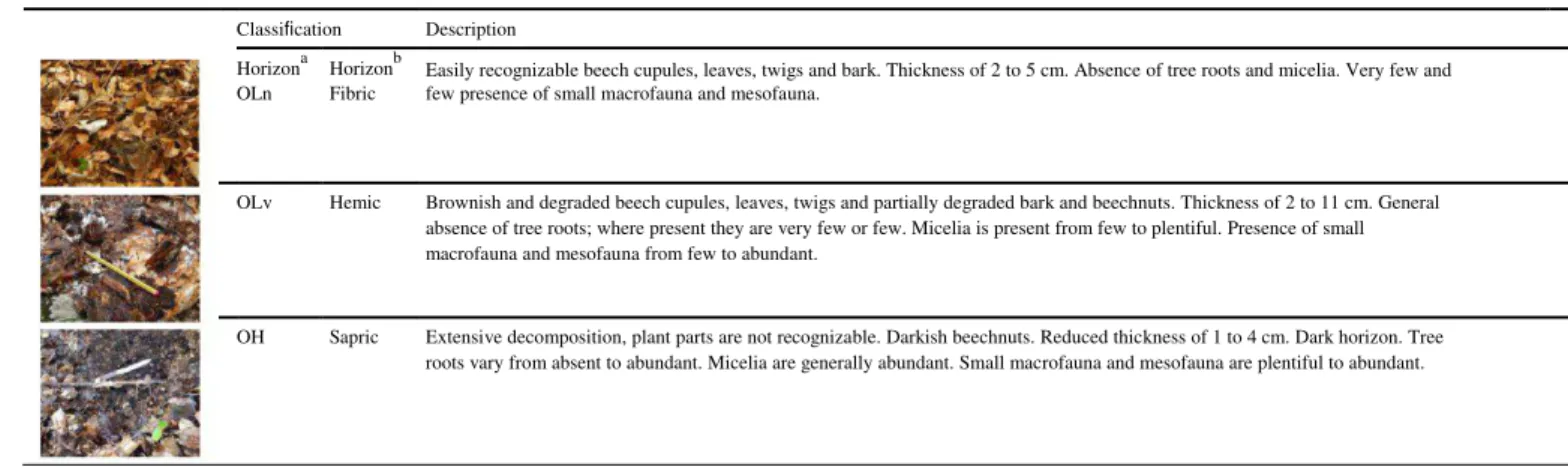
Table 1 - General description of the different types of organic horizons collected divided by study sites. For symbols see legend. a, b
Italy
Study site: Central Apennines - Mount Acuto, Mount San Vicino, and Mount Terminillo. Classification Description
Horizona Horizonb Easily recognizable beech cupules, leaves, twigs and bark. Thickness of 2 to 5 cm. Absence of tree roots and micelia. Very few and OLn Fibric few presence of small macrofauna and mesofauna.
OLv Hemic Brownish and degraded beech cupules, leaves, twigs and partially degraded bark and beechnuts. Thickness of 2 to 11 cm. General
absence of tree roots; where present they are very few or few. Micelia is present from few to plentiful. Presence of small
macrofauna and mesofauna from few to abundant.
OH Sapric Extensive decomposition, plant parts are not recognizable. Darkish beechnuts. Reduced thickness of 1 to 4 cm. Dark horizon. Tree
roots vary from absent to abundant. Micelia are generally abundant. Small macrofauna and mesofauna are plentiful to abundant.
Texas
Study site: Lubbock - North Fork of the Brazos River; Houston - George Bush Intercontinental Airport, WG Jones State Forest, San Jacinto River and Sam Houston National Forest. Classification Description
Lubbock
Horizona Horizonb Organic layer originated by deposition after an alluvial event. Recognizable branches, leaves, with a predominance of twigs and OLn Fibric bark. Spot with accumulation of grass leaves. Thickness of 4 to 6 cm. No roots and micelia. No small macrofauna or mesofauna
activities.
OLv Hemic Brownish and darkish degraded vegetal material made by not easily recognizable leaves, twigs, and bark. Thickness from 5 to
10 cm. Roots and micelia are not present. Very few and few presence of small macrofauna and mesofauna.
Houston
OLn Fibric Non-decomposed pine leaves, pine cones, twigs and bark. Thickness of 1 to 5 cm. Absence of root and micelia. Few presence of
small macrofauna and mesofauna.
OLv Hemic Brownish and pressed recognizable pine leaves, bark, and twigs. Thickness of 2 to 6 cm. General presence of tree roots from very
few to few. Micelia generally goes from very few to abundant, with spots of very abundant presence. Considerable small
macrofauna and mesofauna activities.
OH Sapric Extensive decomposition, plant parts are not recognizable. Thickness of 1 to 2 cm. Tree roots vary from absent to few. Micelia is
reduced from very few to plentiful. Small macrofauna and mesofauna are plentiful to abundant.
New Mexico
Lincoln County - Lincoln National Forest.
Classification Description
Horizona Horizonb Not decomposed pine and deciduous leaves, pine cones, twigs, and bark. In spots, woody parts of bark from degradation of dead OLn Fibric trees. Thickness of 1 to 7 cm. Absence of roots and micelia. The presence of degraded tree parts induces a considerable presence of
small macrofauna and mesofauna, in general absent or few.
OLv Hemic Degraded pine leaves and deciduous twigs, presence of pine cones. Degraded barks reduced in fine dust, structure not
recognizable. Brownish horizons. Thickness of 1 to 8 cm. Few roots. Micelia generally goes from few to plentiful. Considerable
small macrofauna and mesofauna activities.
OH Sapric
Vegetal material completely decomposed, only pine cones are still recognizable. Thickness from 2 to 3 cm. Generally few tree roots. Micelia is few to plentiful. Small macrofauna and mesofauna are plentiful to abundant
(continued on next page)
.
a Horizon designation per Association française pour l'Etude du sol (2008).
132 V. Cardelli et al. / Geoderma 288 (2017) 130–142
Recently, several studies have investigated rapid, inexpensive, and non-destructive methods, such as visible near infrared diffuse reflectance spectros-copy (VisNIR-DRS) and portable X-ray fluorescence spectrometry (PXRF) for soil analysis (Horta et al., 2015; Weindorf et al., 2014). These proximal sensing methods have become increasingly accurate and widely accepted offering data in situ in seconds given virtually no pre-processing requirements (Viscarra Rossel et al., 2006a, 2006b), with substantive advantages over traditional laboratory-based techniques. VisNIR-DRS is a spectrometric method which uses wavelengths across visible and near infrared regions (350–2500 nm) to explore the interaction between incident radiation and reflectance off of the soil surface; absorption is facilitated by C-H, N-H, or O-H bonds within the matrix (Chang et al., 2005). Due to this characteristic, it is highly applicable to C and N determination in soils. However, VisNIR-DRS spectra are generally weak, non-specific, and somewhat broad in their extent because of overlapping spectral signatures arising from variable soil components (Stenberg et al., 2010). As such, the instrument alone does not provide sufficient accuracy for complete soil characterization (Morgan et al., 2009). In fact, others have suggested the application of VisNIR-DRS in tandem with other sensing technologies (Brown et al.,2006; Fajardo et al., 2015). A complementary technique, PXRF, provides a multi-elemental analysis with a large range of quantification from low mg kg−1 to 100% for many elements (Hettipathirana, 2004). However, elements with stable electron configuration and low fluorescent energy (e.g., Na, N, H, Li, C) are not detectable (Wang et al., 2015). Nonetheless, several recent studies (e.g., Aldabaa et al., 2015; Chakraborty et al.,2015; Wang et al., 2015) have shown compelling predictive accuracy by combining the spectral signature of VisNIR-DRS with elemental data from PXRF, the latter used as auxiliary input data into the original advanced regression model. Individual or combined use of these two instruments allows for characterization of multiple soil parameters to include SOM (Stenberg et al., 2010), total carbon, total nitrogen (Wang etal., 2015), total phosphorus (Hu, 2013), cation exchange capacity(Sharma et al., 2015), pH (Sharma et al., 2014), salinity, (Swanhart etal., 2014), texture (Zhu et al., 2011), and contaminants (Chakraborty et al., 2015; Horta et al., 2015; Paulette et al., 2015). While the afore-mentioned studies offer wide-ranging application, most were conducted on mineral soils with limited organic content. Comparatively less information is available on the use of combined proximal sensors for soil organic layer (O horizon) characterization. Wang et al. (2015) evaluated total carbon and nitrogen via combined PXRF and VisNIR-DRS approaches, but did so on mineral soils, lacking any analysis of true organic horizons. Similarly, Chang and Laird (2002) have shown the efficacy of VisNIR-DRS to characterize soil carbon, but again, the soils evaluated were largely mineral soils. McWhirt et al. (2012) used a single sensor approach (VisNIR-DRS) to characterize the organic matter content of compost products. While organic, composted products differ substantively in their physicochemical composition from that of organic soils. By contrast, the present study explicitly aims to evaluate the combined use of both proximal sensors (PXRF and VisNIR-DRS) in characterization of organic soil horizons in variable states of decay. As such, the objectives of this study were to: 1) quantify total carbon and nitrogen in natural organic soils by VisNIR-DRS and PXRF individualistically and, 2) explore if there is a benefit in predictive accuracy from concatenating VisNIR-DRS spectra and PXRF elements. We hypothesize that total carbon and nitrogen of largely organic horizons can be directly predicted from the reported PXRF elements and VisNIR-DRS spectra. We further hypothesize that either a fused model or a model averaging approach will produce better predictability than either the VisNIR-DRS or the PXRF approach independently.
2. Materials and methods 2.1. General occurrences and features
In sum, 136 organic laden samples from non-saturated, uplands were collected in Italy and United States of America (Texas and New Mexico) during 2014 and 2015; a few mineral laden soils were also included as part of this dataset as a link to previously established work on mineral soils. The sites
differed substantively in their geological composition, soil development, climate, and vegetation.
In Italy, a total of 39 organic horizons were collected from forest soils across three different sites on the Apennines chain (central Italy): Mount Acuto, Mount San Vicino, and Mount Terminillo. The soils developed from limestone of different geological origin: Mount Acuto is characterized by limestone (Lower Cretaceous - Aptian), Mount San Vicino is grey limestone with traces of flintstone and marl from the Jurassic (Lias) Pliensbachian Sinemurian and Mount Terminillo is grey limestone with trace amounts of flintstone (Jurassic Toarcian-Sinemurian) (ISPRA, 2015). The soils of these areas are classified as Mollisols or Inceptisols (Soil Survey Staff, 2014), characterized by a mesic soil temperature regime (10 °C to 12 °C) along with an udic soil moisture regime (from 825 mm to 1430 mm precipitation). In the three areas, the cover vegetation was mainly composed of Fagus sylvatica from 80 to 99%, with Carpinus betulus at Mount Acuto, Quercus cerris, Castanea sativa, and Sorbus aria at Mount San Vicino, and Laburnum anagyroides and Acer spp. at Mount Terminillo.
In Texas, 16 alluvial organic samples were collected in backwater areas along the North Fork of the Brazos River in Lubbock County in major land resource area (MLRA) 77C - Southern High Plains - Southern Part (Soil Survey Staff, 2006). Soils of this MLRA are generally developed by eolian deposits in the Blackwater Draw Formation of Pleistocene age, classified as Alfisols, Inceptisols, Mollisols, and Vertisols, and have a thermic soil temperature regime (13 °C to 17 °C) and an ustic soil moisture regime (from 405 to 560 mm precipitation). Mostly short and mid-prairie grasses and scanty tree and shrubs (e.g., Bouteloua gracilis, Bouteloua dactyloides, Bouteloua curtipendula) are prevalent. Separately, 27 various organic horizons were sampled in forested areas of the George Bush Intercontinental Airport, WG Jones State Forest, San Jacinto River, and Sam Houston National Forest; all generally in the vicinity of Houston, Texas. The WG Jones State Forest, San Jacinto River, and Sam Houston National Forest occur in MLRA 133B - Western Coastal Plain (Soil Survey Staff, 2006), where soils developed from Tertiary and Cretaceous marine sediments consisting of interbedded sandstone, siltstone, shale and loose primary particles. In particular, the Reklaw and Weches Formations in the Claiborne Group form the Redland area of East Texas. The main soil orders in this MLRA are Alfisols and Ultisols with a thermic soil temperature regime (16 °C to 20 °C), an udic or aquic soil moisture regime (990 to 1600 mm precipitation). Vegetation of the area is typified by pine-hardwood species such as Pinus taeda, Pinus echinata, Liquidambar styraciflua, Quercus falcate, and Cornus flor-da; Callicapra americana, and Smilax spp. are common in the woody understory. Schizachyrium scoparium and Bothriochloa barbinodis are the dominant herbaceous species. Of the 27 samples collected in this area, four were collected in densely wooded pine forests adjacent to George Bush Intercontinental Airport, which is a few kilometers beyond the aforementioned MLRA boundary, but quite similar in the organic horizons sampled.
In New Mexico, 54 samples were collected near the periphery of the Lincoln National Forest of Lincoln County; the horizons sampled were dominantly organic, but a few transitioned into organic laden mineral soils. The area is in MLRA 39-Arizona and New Mexico Mountains (Soil Survey Staff, 2006). The area is characterized by Cenozoic volcanic rock and various sedimentary sections of the Colorado Plateau. The southern and eastern parts contain Permian and Cretaceous sedimentary rock over a Precambrian granite core. Main soil orders of this MLRA are Inceptisols, Mollisols, Alfisols, and Entisols, with mainly frigid or mesic soil temperature regimes (2 °C to 13 °C) and an ustic/udic mois-ture regime (358 mm to 760 mm precipitation). Pinus ponderosa occurs is the dominant vegetation in the low and intermediate heights, while at higher altitudes, Picea abies and Pseudotsuga menziesii are commonplace.
V. Cardelli et al. / Geoderma 288 (2017) 130–142 133
2.2. Field sampling
For maintaining an extensive variation in terms of physicochemical characteristics, composition and origin, samples were randomly collected within morphologically established, organic laden horizons. Almost all samples were classified as O horizons according to Baize and Girard(2008). The different stages of degradation were classified as: i) OL,consisting of leaf debris with little or no degradation (b10% of fine or-ganic matter) whereby the botanic origin was easily recognized; sub-horizons were recognized as OLn, fresh litter with minimal degradation, and OLv, where the plant material was subject to initial degradation such as changes in color, volume, and inter-particle linkages; and ii) OH, with N70% of fine organic (humic) material following extensive decomposition (Table 1). The latter is homogenous, massive, and reddish-brown to black in color with an abundance of fine roots. These three states of decomposition are roughly akin to fibric, hemic, and sapric materials as defined by the Soil Survey Staff (2014), respectively.
2.3. Laboratory characterization and VisNIR scanning
Soil samples were air dried and ground to <1 mm prior to chemical analyses and spectral scanning. Total C (TC) and total N (TN) were de-termined by a TruSpec® dry combustion analyzer (LECO Corp., MI, USA) according to Dumas method combustion (Nelson and Sommers,1996).
Spectral reflectance values of air dried and ground soil samples were measured proximally over the VisNIR region (350–2500 nm) by a portable PSR-3500® VisNIR spectroradiometer (Spectral Evolution, USA). The reflectance data were resampled to 1 nm output values. Scanning was done with a contact probe containing a 5 W halogen lamp, minimizing errors associated with stray light during measurements. Each sample was uniformly tiled in a glass petri plate and scanned four times, physically repositioning the probe prior to each scan. The mean of 10 internal scan over 1.5 s produced one individual scan. The spectroradiometer was standardized after every two samples using a NIST certified white reference. The average spectral curve was calculated and further used for spectral preprocessing and subsequent predictive modeling.
Necessary treatments of raw average reflectance spectra were done in R version 2.11.0 (R Development Core Team, 2008) following the spline fitting methods outlined in Wang et al. (2015). The spectral pre-processing involved converting reflectance to absorbance by log(1/R) which was executed in the Unscrambler®X 10.3 software (CAMO Soft-ware Inc., Woodbridge, NJ).
2.4. Scanning with PXRF
A DP-6000 Delta Premium portable X-ray fluorescence (PXRF) spec-trometer (Olympus, Waltham, MA, USA) facilitated sample scanning. Configured with a Rh X-ray tube, the instrument was operated at 15– 40 kV; an integrated ultra-high resolution (165 eV) silicon drift detector quantified each element detected. Before scanning, a 316 alloy clip was used to standardize the instrument. Primary analysis was conducted in Soil Mode (three beams of 30 s each); it can detect the following: Ag, As, Ba, Ca, Cd, Cl, Co, Cr, Cu, Fe, Hg, K, Mn, Mo, Ni, P, Pb, Rb, S, Sb, Se, Sn, Sr, Ti, V, Zn, and Zr. A second scanning was performed with Geochem Mode (two beams of 30 s each) in order to measure Mg, S, Al, and Si. Geochem and Soil Mode scans were done in duplicate, with the spectrometer physically repositioned between each scan. Sample homogeneity was ensured during the grinding step. Data were then averaged between scans to obtain a mean of elemental data for each sample. Data quality was ensured via the scanning of two NIST certified reference samples, with recovery percentage calculated as PXRF reported vs. NIST certified values. Results were as follows (PXRF reported/NIST certified [recov-ery]): Zn 4263/4180 mg kg−1 [1.02]; Cu 3559/3420 mg kg−1 [1.04]; K 27,081/21,700 [1.25]; Ca 9119/9640 mg kg−1 [0.95]; Ti 3540/ 3110 mg kg−1 [1.14]; Mn 2237/2140 [1.05]; Fe 50,574/ 43,200 mg kg−1 [1.17]; As 1639/1540 mg kg−1 [1.06]; Sr 269/255 [1.05]; Pb 5608/5520 [1.02].
2.5. Data mining
We performed all statistical modeling via R version 2.11.0 (R Development Core Team, 2008) software. We also checked the normality of residuals by the Shapiro-Wilk test at a 5% significance level. In the present study, both original TC and TN values were negatively skewed (Pearson skewness coefficient −1.78 and −0.37 for TC and TN, respectively), while Box–Cox conversion (Box and Cox, 1964) using λ = 0 (log10 transformed) was unable to conform normal distribution. Principal component analysis (PCA) was executed via R version 2.11.0 using the ‘prcomp’ function to visualize spectral behavior of soil samples from different geographical areas and organic horizons. Optimal number of principal components (PC) was decided from a screeplot.
In this study, the whole dataset was split into 70% calibration (n = 96) and 30% validation set (n = 40) using the Kennard-Stone algorithm (Kennard and Stone, 1969), which is an adaptive procedure to select the most representative samples based on Euclidean distance. Calibration samples were used to establish a prediction model, whereas validation samples were used to assess the model's predictive ability (Chen et al.,2015). Initially, we targeted both TC and TN with VisNIR-DRS spectraonly via partial least squares regression (PLS), elastic net regression (ENET), penalized spline regression (PSR), and random forest regression (RF) (Breiman, 2001; Guyon et al., 2002; Viscarra Rossel et al., 2006b). Additionally, both TC and TN were predicted with PXRF elemental data via PLS, ENET, and RF models.
Regularized methods, which play an important role in both statisti cal and data mining problems, can be described as Eq. (1):
(1)
where L(Y, Xβ) is a non-negative loss function, J(β) is a non-negative penalty on the model complexity and λ is the non-negative tuning parameter. The key idea for regularized methods is to balance between the goodness-of-fit on the training data and the complexity of the model. Usually, a complicated model always shows a good fit to the calibration data. Nonetheless, this commonly leads to problems of overfitting, where the model is too adapted to the training data and often has a poor prediction performance on new samples.
Elastic net, devised by Zou and Hastie (2005) is a regularized regression method that linearly combines the ridge penalty and the least absolute shrinkage and selection operator (LASSO) penalty (Eq. (2))
134 V. Cardelli et al. / Geoderma 288 (2017) 130–142
where SSE is the sum of squared errors, ∑|βj | is the LASSO penalty, and ∑β2j is the ridge penalty. In high dimensional data analysis where many predictors are correlated to each other, the LASSO penalty tends to pick a few of the predictors and discard the others (sparse model), while the ridge penalty shrinks the coefficients of correlated predictors towards each other (dense model). The ENET penalty combines these two penalties so that when the predictors are correlated in groups, it will produce a sparse model with good prediction performance, while boosting a grouping effect. Another advantage of ENET is that it can handle the high dimension and low sample size problem. In this study, ENET was run using the ‘glmnet’ package in R, produced by Friedmanet al. (2015). Details of PSR and RF methodology are summarized in Wang et al. (2015).
2.6. Model fusion and model averaging
Model fusion and model averaging (model ensemble) were tested to determine if combination of the predictions for the VisNIR-DRS and PXRF models into a single composite score could improve predictive accuracy of TC and TN. Initially, three fused modeling approaches (PSR + RF), (PLS + RF) and (ENET + RF) were employed where PSR/PLS/ENET were used to fit the training set (containing VisNIR-DRS spectra only). Next, we ran the RF using the PSR/PLS/ENET residual as the response and PXRF elements as the predictors (Chakraborty et al., 2015). Succinctly, the prediction value on the validation set using (PSR + RF), (PLS + RF) and (ENET + RF) contains two additive parts: the prediction from PSR/PLS/ENET model using the VisNIR-DRS spectra plus the prediction from RF model using the PXRF data. An outline of this fused procedure is shown in Fig. 1.
For model averaging we used Granger-Ramanathan averaging (GRA) (Granger and Ramanathan, 1984) with some modifications. The GRA approach requires fitting a multivariate linear regression model where lab measured soil property values are regressed against the corresponding predictions derived from VisNIR-DRS and PXRF models. Initially, the PSR/PLS/ENET model was fitted on the calibration set (n = 96) using the VisNIR-DRS spectra. Subsequently, the RF model was fitted using only PXRF elements as predictors and TC or TN as the response. Note that this RF model was not the same as the RF model in fused approaches (PSR + RF, PLS/RF, or ENET + RF) as the latter used residual as
a response. Next, a bivariate linear regression was fitted with Eq. (3):
Y = a + b * X + c * Z (3)
where Y is either TC or TN on calibration set; X is the fitted value (on cal-ibration set) from the PSR/PLS/ENET model; Z is the fitted value (on the calibration set) from the RF model; a is the intercept; b is the estimated model weight for the PSR model; and c is the estimated weight for the RF model. To predict the validation set (n = 40), we first generated the prediction value, X*, from the PSR/PLS/ENET model, and prediction value, Z*, from the RF model. The GRA prediction is given as Eq. (4):
Y = a + bX* + cZ (4)
We followed the Kennard-Stone splitting scheme for both fused models and GRA.
2.7. Whole geographical area and organic horizon holdout validation Further, whole geographical area and organic horizon holdout validations were executed for both TC and TN to determine how area to area and horizon to horizon heterogeneity affected prediction accuracies (Brown et al., 2005). Whole-geographical area holdouts were achieved by calibrating a model using the best performing algorithm with three geographical areas and then validated using the fourth area. Moreover, whole-organic horizon holdouts were achieved by calibrating a model using the best performing algorithm with two organic horizons and then validated using the third organic horizon.
In this study, the root mean square error (RMSE), regression coefficient (R2), residual prediction deviation (RPD) (Eq. (5)), bias, and ratio of performance to interquartile distance (RPIQ) (Eq. (6)) were used to evaluate model performance (Gauch et al., 2003 Bellon-Maurel et al., 2010). RPD based model accuracy classification scheme devised by Chang et al. (2001) was followed for evaluating model accuracy.
(5)
(6)
where, Yobs and Ypred are the observed and predicted response variables, respectively, Ymean is the average of the Yobs values, and n denotes the sample number in the validation data set. RPIQ was defined as IQ/SEP, where SEP represents the standard error of prediction, and IQ denotes the interquartile distance of the validation set (IQ = Q3–
Response: TC and TN values
Final predicted value: Y PSR/PLS/ENET + Y RF
Y PSR/PLS/ENET Y RF Response:
Residuals
PSR/ PLS/ ENET modelling RF modelling
Input: Spectral data Input: PXRF data
V. Cardelli et al. / Geoderma 288 (2017) 130–142 135
Table 2 Table 3
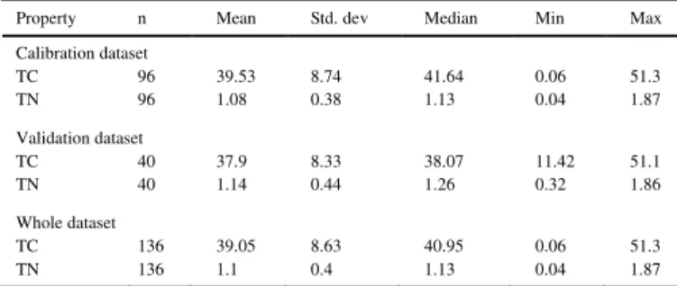
Summary statistics of soil properties. Validation statistics of multivariate models based on Kennard-Stone splitting. Property n Mean Std. dev Median Min Max
Calibration dataset TC 96 39.53 8.74 41.64 0.06 51.3 TN 96 1.08 0.38 1.13 0.04 1.87 Validation dataset TC 40 37.9 8.33 38.07 11.42 51.1 TN 40 1.14 0.44 1.26 0.32 1.86 Whole dataset TC 136 39.05 8.63 40.95 0.06 51.3 TN 136 1.1 0.4 1.13 0.04 1.87
Q1). In this study, optimal model performance featured low RMSE values along with high RPD, R2, and RPIQ.
3. Results and discussion 3.1. Soil properties and PCA
Statistical moments for TC and TN measured on the soil samples used in the regression models are listed in Table 2. Soil TC and TN showed negatively skewed distribution with mean concentrations of 39.05% and 1.10%, respectively for the whole dataset; 39.53% and 1.08%, respectively for the calibration set; and 37.90% and 1.14%, respectively for the validation set. Of the 13 elements obtained by the PXRF soil mode, only nine [Zn, S, K, Ca, Ti, Rb, Mn, Fe, Sr] were suitable for use in the multivariate predictive models with continuous data across all samples scanned. Within-region variability of TC and TN exhibited substantial variation. For instance, in Italy sample TC ranged from 28.06% to 45.94%. Showing similar variation, Lubbock samples showed TC ranging from 25.93% to 41.20%. Comparatively higher variability was observed for Houston samples (11.42– 48.54%), while maximum TC variability was observed in samples from New Mexico region (0.06–51.30%). Lubbock samples showed TN ranging from 1.13–1.60%. Comparatively higher variability was observed for Italy (0.80– 1.87%) and Houston samples (0.30–1.47%). Following a similar trend of TC, maximum variability in TN was observed from New Mexico soils (0.04– 1.87%). Overall, variability in estimated TC and TN was due largely to the variability in the parent material, climate, C source, land use, and vegetation cover. However, the extent of variability appeared related with the range of the mean annual soil temperature of the considered sampling area, the highest in the New Mexico soils (2–13 °C), the lowest in the Italy
Soil
property PLS RMSE
(%) Approach Model R2 LFa (%) RPD Bias RPIQ Total C VisNIR DRS PSR 0.80 – 3.46 2.40 0.15 3.02 PLS 0.82 14 3.27 2.52 −0.15 3.23 ENET 0.73 – 4.24 1.96 0.53 2.50 RF 0.60 – 5.14 1.62 −0.03 2.06 PXRF PLS 0.53 5 5.59 1.49 0.89 1.89 ENET 0.62 – 5.03 1.65 0.04 2.10 RF 0.58 – 5.30 1.57 0.20 2.00 VisNIR PSR + RF 0.87 – 3.01 2.75 0.31 3.50 DRS + PXRF PLS + RF 0.89 14 2.94 2.84 0.22 3.60 ENET + RF 0.79 – 3.73 2.23 0.56 2.84 GRA PSR.RF 0.59 – 5.27 1.58 −0.13 2.01 PLS.RF 0.60 14 5.15 1.62 −0.13 2.06 ENET.RF 0.62 – 5.05 1.65 −0.11 2.10 Total N VisNIR DRS PSR 0.81 – 0.178 2.46 0.03 3.80 PLS 0.75 13 0.214 2.01 0.03 3.25 ENET 0.74 – 0.221 2.00 0.05 3.14 RF 0.61 – 0.271 1.62 −0.01 2.56 PXRF PLS 0.28 4 0.492 0.89 0.02 1.41 ENET 0.32 – 0.356 1.23 0.01 1.95 RF 0.57 – 0.285 1.54 0.01 2.43 VisNIR PSR + RF 0.85 – 0.160 2.62 0.03 4.12 DRS + PXRF PLS + RF 0.82 13 0.191 2.30 0.05 3.59 ENET + RF 0.78 – 0.203 2.17 0.06 3.42 GRA PSR.RF 0.79 – 0.197 2.22 0.03 3.51 PLS.RF 0.64 13 0.262 1.68 0.02 2.65 ENET.RF 0.65 – 0.256 1.71 0.03 2.70 a
PLS LF, partial least squares latent factor.
soils (10–12 °C), intermediate in the other two subsets (16–20 °C in the Houston soils, and 13–17 °C in the Lubbock soils).
Levene's test yielded equality of variance of TC and TN values among the training and test sets (p = 0.65 and 0.55 for TC and TN, respective-ly). Moreover, t-test could not establish a significant difference between mean TC (p = 0.53) and TN (p = 0.51) for these two data sets. These results indicated that the validation samples based on the Kennard-Stone method can properly represent the studied population. The first two leading PCs constituted over 95% of the spectral variation (Fig. 2a). Although some overlapping among samples from four regions were discernible from the PC1 vs. PC2 plot, these regions had different ranges, shapes, and distributions in the spectral space, indicating variable SOM composition from different organic input sources (Fig. 2b). Moreover, the PCA plot indicating samples from three different organic horizons (OH, OLn and OLv) (Fig. 2c) indicated that OH horizon samples
Fig. 2. Plots showing a) “Screeplot” of the first 10 principal components (PCs), b) pairwise PC plots of the first two components using VisNIR DRS first derivative spectra indicating four different geographical areas and c) pairwise PC plots of the first two components using VisNIR DRS first derivative spectra indicating three different organic horizons. Lines represent convex hulls and colored dots represent centroids of datasets from four different geographic areas. ITA, LBB, HOU and NMX represent samples from Italy, Lubbock, Houston and New Mexico regions, respectively. (For interpretation of the references to color in this figure legend, the reader is referred to the web version of this article.)
136 V. Cardelli et al. / Geoderma 288 (2017) 130–142
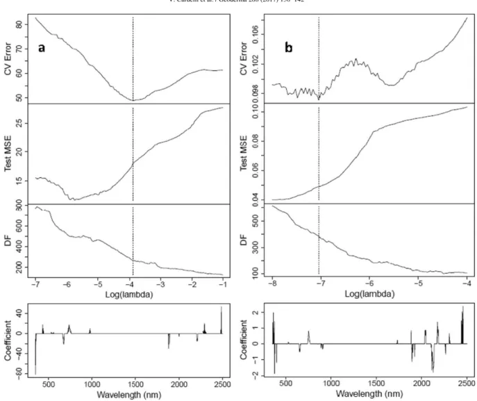
Fig. 3. Parsimony features of ENET for a) TC and b) TN. CV error, MSE, DF and λ represent cross-validation error, test error, the number of selected wavelengths and the parameter to tune the parsimony of the model, respectively.
were quite different from the samples from OLn and OLv horizons. The OH horizon samples tended to have larger values on the PC1 scores. Contrarywise, the samples from the OLn and OLv horizons were relatively close. Notably, the samples from the OLv horizon tended to have relatively larger PC2 values while there was an obvious outlying sample with the largest PC1 value and smallest PC2 value.
3.2. Validation results and model parsimony
In fused models, both TC and TN were estimated with good RPIQ values, better than using an individual instrument or GRA (Table 3), which has been noted before elsewhere (Wang et al., 2015). Fused (PLS + RF) and (PSR + RF) models yielded the highest RPDs for TC (2.84) and TN (2.62), respectively. While RPD values for both tested soil properties dropped in (ENET + RF) fused models, they still explained nearly 80% of the TC and TN variability. Overall, all three fused models of TC showed similar accuracies (Table 3), as reported for soil organic C in the review of Soriano-Disla et al. (2014) where the median R2 of validations was calculated as 0.83 (33 studies).
Wavelength selection not only enhances the stability of the model but also makes the model more parsimonious. Although (PSR + RF) yielded the lowest RMSE for TN (0.160%), both PSR and RF are not parsimonious models since they do not select the subset of important variables. Although for RF it is possible to select different mtry values, which is the size of the candidate subset for each splitting, models
with different mtry values still select all the variables. Despite controlling the smoothness of the neighboring coefficients through λ, PSR is also unable to select important wavelengths. Fig. 3 illustrates parsimony features of ENET for TC (Fig. 3a) and TN (Fig. 3b) where cross-validation error, test error (mean squared error or MSE), and the degrees of freedom (DF) (the number of selected wavelengths in the ENET model) were plotted against log of λ which is the parameter to tune the ENET parsimony. Note that the larger the λ, the more parsimonious the model. The vertical dash line shows the optimal λ that minimizes the cross-validation error. The bottom plot shows the ENET coefficient plot against the VisNIR wavelengths. For both soil properties, most of the coefficients were zero, indicating that they were not selected into the model. Additionally, based on the DF plots, it was evident that the optimal TC and TN models selected only ~300–350 out of 2151 wavelengths. Conversely, using a fused (PLS + RF) model on the reduced feature sets (14 and 13 latent factors for TC and TN, respectively) returned the best result for TC and slightly higher RMSE for TN (0.191%) than (PSR + RF) (0.160%) (Table 3). Based on these observations, we conclude that while considering both model precision and parsimony, (PLS + RF) emerged as the best model for both TC and TN.
For both TC and TN, while utilizing VisNIR-DRS or PXRF alone, RF and PLS models yielded the largest validation RMSE values, respectively, and were therefore the least precise (Table 3). In general, PXRF measurements were poorly correlated to both TC and TN, suggesting its limitation to make full geochemical assessment alone due to its inability to
V. Cardelli et al. / Geoderma 288 (2017) 130–142 137
RMSE=3.46%
RMSE=3.01 %
RMSE=3.27 % RMSE=2.94 %
RMSE=4.24 % RMSE=3.73 %
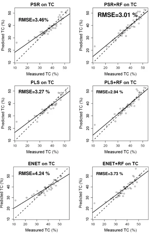
Fig. 4. Plots of observed vs. model predicted (VisNIR DRS only and fused) TC values using the validation set (with dotted 1:1 line).
handle low concentrations and light elements (Z ≤ 11) (Weindorf et al.,2008). Among the nine elements used in predictive models, only Al(1.48%), Ca (2.53%) and Si (4.83%) were present in high concentrations, while the other six elements were present at low levels (b1%). Thus, it seemed prudent to calibrate using PXRF spectra instead of elements if high accuracy is desired. While GRA substantially worsen the validation results for TC, (PSR + RF) model averaging for TN yielded close RMSE (0.197%) to those produced by fused models. The reasonably good performance of PSR in all three approaches (VisNIR only, fused, and GRA) can be attributed to the fact that in case of ‘fat’ data (large number of di-mensions and small sample size) PSR uses all samples and smooths constraints on the coefficient. Therefore, PSR often works well on signal
regression problems which are usually strongly dimensional and have a relatively small sample size.
As coefficients of determinations of TN were rather similar to those of TC using VisNIR-DRS in isolation, we conclude that VisNIR-DRS sensed a grouping of soil components comprising organic functional groups that contain organic N fractions (Wang et al., 2015) (Table 3). Moreover, both TC and TN are spectrally active components or chromophores, which absorb incident energy at discrete energy levels and show broad and weak absorption features in the VisNIR region (Ben-Dor, 2011) Although intense VisNIR-DRS spectral bands cannot be di-rectly ascribed to metals or other components, Song et al. (2012) revealed that metals can interact with chromophores such as soil C.
138 V. Cardelli et al. / Geoderma 288 (2017) 130–142
RMSE=0.160% RMSE=0.178%
RMSE=0.214 % RMSE=0.191%
RMSE=0.221% RMSE=0.203%
Fig. 5. Plots of observed vs. model predicted (VisNIR DRS only and fused) TN values using the validation set (with dotted 1:1 line).
However, S was negatively correlated with TC (ρ = −0.48); likely since S is very light with an atomic mass of 16 and was present in low concentrations (max = 0.43%).
Plots of observed vs. model predicted (VisNIR-DRS only and fused) TC and TN values are presented in Figs. 4 and 5, respectively. In general, all models showed overestimation at lower TC or TN values and under-estimation at higher values. Several of these overunder-estimations occurred because of the relative scarcity of observations with low values, which was expected since the samples came dominantly from organic horizons. Another possible explanation for TC and TN prediction errors is undecomposed organic matter and variable C sources, as noted before elsewhere (Henderson et al., 1992). Indeed, the VisNIR-DRS spectra
for SOM have not been fully defined yet, because of the complexity or unclear definitions of these materials (Brown et al., 2006). Probably the TC and TN predictability could have been enhanced by using soil management or vegetation specific models (Morgan et al., 2009); nonetheless, exploring this notion was beyond the scope of this study.
3.3. Model fusion vs. model averaging
It was apparent that GRA model averaging by combining the VisNIR-DRS and PXRF predictions for consolidated use could not produce better accuracy than model fusion. In practice, “good” model averaging should contain the models that complement each other. In fused models, RF
V. Cardelli et al. / Geoderma 288 (2017) 130–142 139
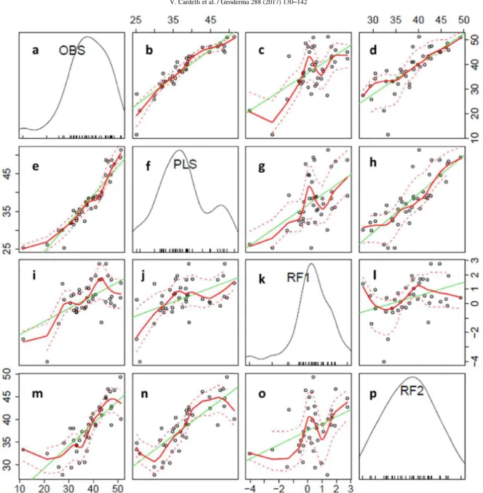
Fig. 6. Diagnostic scatter plot matrix showing density plots for four competitors: observed TC values (OBS), RF in (PLS + RF) fused model (RF1) and RF in GRA (RF2). Black circles represent validation samples. The green and red solid lines are the fitted linear regression line and the loess smoother fit, respectively. The red dash lines represent one standard error above and below the estimated function. For diagonal plots, the vertical axis shows the density function for its corresponding values. For example, panel a is the density plot of TC while the tickmarks at the bottom axis show the observed values in the data. In the off-diagonal plots, their axes are all in the % unit. For example, panel e shows the scatter plot of observed TC % (on the vertical axis) and predicted TC % values from PLS model (on the horizontal axis) using spectral data. (For interpretation of the references to color in this figure legend, the reader is referred to the web version of this article.)
was fitted based on the PLS/PSR/ENET residuals. The sequential fitting in PLS/PSR/ENET + RF allowed the RF model to complement the former. Conversely, combining PLS/PSR/ENET and RF in parallel fashion through GRA (namely, separately on VisNIR-DRS and PXRF) produced incompat-ibility. Succinctly, they perhaps made the same mistake on the same sample. To justify this postulation and clearly visualize the prediction improvement by using the fused models, Fig. 6 represents a scatterplot matrix produced in R using the spm function in the car library, taking the PLS + RF model as an example. The diagonal elements are the density plots for the four competitors [observed TC values (OBS), RF in (PLS + RF) fused model (RF1), and RF in GRA (RF2)]. For example, the upper left one is the density plot of TC while the tickmarks at the bottom axis show the observed values in the data. The off-diagonal elements are
the pairwise scatter plots of four competitors, together with the best linear and nonlinear smoothers. For example, Fig. 6e shows the scatter plot of observed TC (on the vertical axis) and predicted TC values from PLS model (on the horizontal axis) using spectral data. The green and red solid lines are the fitted linear regression line and the loess smoother (a popular nonlinear smoother using local linear regression) fit, respectively. The red dash lines represent one standard error above and below the estimated function. It can be observed that PLS tended to underestimate the samples with TC values between 30 and 45% and overestimate the samples with TC values <20% through the bending shape of the red loess smoother (Fig. 6e). Interestingly, while RF1 “corrected” the PLS model by lifting the underestimated area (30–45% TC) and lowering the overestimated region (<20% TC) (Fig. 6i), this was not totally