Università Politecnica delle Marche
Scuola di Dottorato di Ricerca in Scienze dell’Ingegneria Curriculum in Ingegneria Civile, Ambientale, Edile e Architettura
---
Elasto-plastic models for the response of
passive rigid piles
Ph.D. Dissertation of: Caferri Leonardo Tutor:
Prof. PASQUALINI ERIO
Co-tutor:
Prof. BELLEZZA IVO
Curriculum Advisor:
Prof. LENCI STEFANO
Università Politecnica delle Marche
Dipartimento di Ingegneria Civile, Ambientale, Edile e Architettura
v
ABSTRACT
The use of piles to stabilise active landslides or to prevent future instabilities has been successfully applied in the past and is nowadays a widely accepted technique. However, while the stabilising piles are usually designed with the aim of reducing the soil displacement rate, the design strategies commonly adopted in engineering practice apply to the ultimate state only, not taking into account any realistic interaction mechanism between pile and soil, and are not capable of predicting the effectiveness of the pile and soil displacement magnitude.
The goal of the present investigation is to propose a practical displacement-based numerical methodology for the analysis and design of passive rigid piles in different ground conditions. The developed method considers both a free-head and an unrotated-head rigid pile, embedded in a Winkler type soil and subjected to the sliding of a surrounding soil. The Winkler approach allows to consider a layered soil stratigraphy and to use the horizontal displacement of the surrounding soil as an input to evaluate the associated lateral deflection of the pile as well as the acting shear forces and bending moments in function of the external ground displacement. A FORTRAN computer program has been written to implement the numerical procedure.
The proposed method seems to be suitable for being implemented in traditional Limit Equilibrium Methods or more in general in any decoupled approach method. Moreover, non-dimensional design charts have been developed for simplified soil stratigraphies, in which the required shear force offered by the pile is plotted over the sliding surface depth, as a function of the pile head deflection, the maximum bending moment and the external soil displacement.
vi
LIST OF TABLES
Table 3-1: General normalised expressions for the calculation of a free-head pile deflection ... 26 Table 3-2:General normalised expressions for the calculation of an unrotated-head pile deflection ... 27 Table 3-3: Typical values of nh for cohesive soil ... 29 Table 3-4: Proportionality constants for a passive free-head rigid pile in a two-layered cohesive soil ... 34 Table 3-5: Elastic solutions for a passive free-head rigid pile in a two-layered cohesive soil ... 36 Table 3-6: Proportionality constants for a passive unrotated-head rigid pile in a two-layered cohesive soil ... 43 Table 3-7: Elastic solutions for a passive unrotated-head rigid pile in a two-layered cohesive soil ... 44 Table 3-8: Proportionality constants for a free-head passive rigid pile in a normal-consolidated cohesive soil sliding on a firm layer ... 60 Table 3-9: Elastic solutions for a free-head passive rigid pile in a
normal-consolidated cohesive soil sliding on a firm layer ... 62 Table 3-10: Proportionality constants for a passive unrotated-head rigid pile in a normal-consolidated sliding cohesive soil over a firm layer ... 69 Table 3-11: Elastic solutions for a passive unrotated-head rigid pile in a normal-consolidated sliding cohesive soil over a firm layer ... 70
vii Table 3-12: Proportionality constants for a passive unrotated-head rigid pile in a cohesionless sliding soil over a cohesive firm layer ... 88 Table 3-13: Elastic solutions for a passive unrotated-head rigid pile in a
cohesionless sliding soil over a cohesive firm layer ... 90 Table 3-14: Proportionality constants for a passive unrotated-head rigid pile in a cohesionless sliding soil over a cohesive firm layer ... 96 Table 3-15: Elastic solutions for a passive unrotated-head rigid pile in a
cohesionless sliding soil over a cohesive firm layer ... 97 Table 3-16: Proportionality constants for a passive unrotated-head rigid pile in a three-layered soil... 115 Table 3-17: Elastic solutions for a passive unrotated-head rigid pile in a three-layered soil ... 117 Table 3-18: Proportionality constants for a unrotated-head passive rigid pile in a three-layered cohesive soil ... 124 Table 3-19: Elastic solutions for a passive unrotated-head rigid pile in a three-layered soil ... 125 Table 3-20: Proportionality constants for a passive rigid pile on a cohesionless soil ... 144 Table 3-21: Elastic solutions for a passive rigid pile on a cohesionless soil ... 146 Table 3-22: Proportionality constants for a unrotated-head passive rigid pile on a cohesionless soil ... 152 Table 3-23: Elastic solutions for a unrotated-head passive rigid pile on a
viii Table 4-1: Equations for calculating ultimate lateral load for piles in a two-layer cohesive soil (after Viggiani [23] and Chmoulian [28]) for a pile of length L; pu2 and pu1 are the limit soil resistance in the stable and sliding layers, k=pu2/pu1, βL is the pile length in the sliding layer ... 173 Table 4-2: Threshold soil displacements for all the first yielding cases ... 183 Table 4-3: Yielded regions for the first yielding cases ... 184 Table 4-4: Proportionality constants and elastic solutions for shear forces and bending moments for a passive free-head rigid pile in a two-layered cohesive soil ... 196 Table 4-5: Threshold soil displacements for a homogeneous Gibson soil... 212 Table 4-6: Proportionality constants and elastic solutions for shear forces and bending moments for a passive free-head rigid pile in a non-cohesive soil ... 219 Table 5-1: Expressions for the coefficients of governing equations for failure mode B, B1, BY and B2 ... 232 Table 6-1: Soil properties as assumed in the example ... 265
ix
LIST OF FIGURES
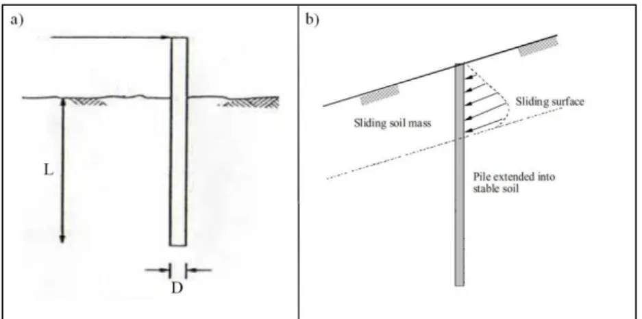
Figure 2-1:Schematic sections of : a) Active pile with length L, diameter D. b) Passive pile embedded in a surrounding sliding soil ... 3
Figure 2-2: Schematic section through a full-height piled bridge abutment
constructed on soft clay [4] ... 4
Figure 2-3: Model for piles in soil undergoing lateral movement [26] ... 12
Figure 2-4: Free-field soil movement [26] ... 12
Figure 2-5: Pile behaviour characteristics for various modes with the hypothesis of constant soil movement in the slide zone, no “drag” zone, pile length of 15m and diameter 0.5m. Sliding soil with Su=30kPa and firm soil with Su=60kPa [26] .... 14
Figure 3-1: a) A beam on an elastic foundation; b) A pile on a bed of springs ... 17
Figure 3-2: Soil reaction p and pile displacement y relationship ... 18
Figure 3-3: A Free—Head rigid and a unrotated-head pile subjected to a soil movement with a generic profile ... 20
Figure 3-4:Distribution of the soil movement: a) generic distribution; b) inverse triangular variation with depth h=0; c)uniform distribution with depth h=1 ... 21 Figure 3-5: Kinematics of rigid piles... 22
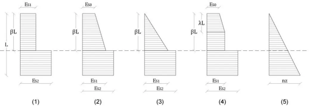
Figure 3-6: Analysed cases: Type-1) Two-layered soil with a constant subgrade reaction modulus. Type 2) Two layered soil with subgrade reaction modulus varying with depth. Type 3) Two layered soil with subgrade reaction modulus varying with depth. Type 4) Three layered soil. Type 5) Homogeneous soil with subgrade reaction modulus increasing with depth ... 27
x
Figure 3-7: Variation of gradient nh, with normalised pile head displacement y0/D,
according to Bhushan et al. [41] and Zhang L. [3] ... 30
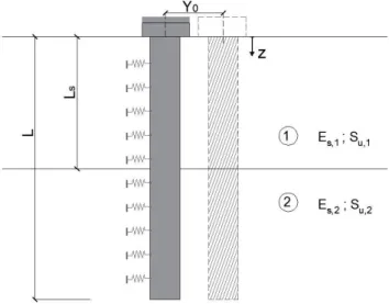
Figure 3-8: Soil profile and pile displacement geometry for a rigid pile in a two-layered cohesive soil ... 31
Figure 3-9: (a) A rigid pile; (b) Variation of Es with depth ... 32
Figure 3-10: Normalised shear force with depth for k=2 and η=1 ... 37
Figure 3-11: Normalised shear force with depth for k=2 and η=0 ... 38
Figure 3-12: Normalised bending moment with depth for k=2 and η=1 ... 39
Figure 3-13: Normalised bending moment with depth for k=2 and η=0 ... 40
Figure 3-14: Soil profile and pile displacement geometry for a unrotated-head rigid pile in a two-layered cohesive soil ... 41
Figure 3-15: Normalised shear force with depth for k=2 and η=1 ... 45
Figure 3-16: Normalised shear force with depth for k=2 and η=0 ... 46
Figure 3-17: Normalised bending moment with depth for k=2 and η=1 ... 47
Figure 3-18: Normalised bending moment with depth for k=2 and η=0 ... 48
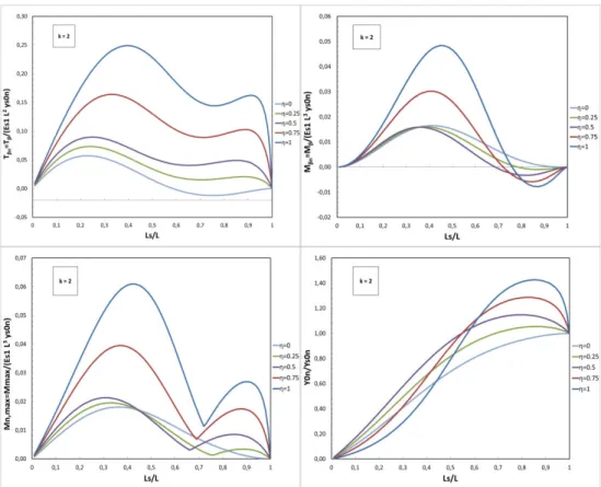
Figure 3-19: Normalised shear force at zn=β, bending moment at zn=β , maximum bending moment and pile head displacement versus Ls/L, for k=2 and different values. Free-head condition ... 52
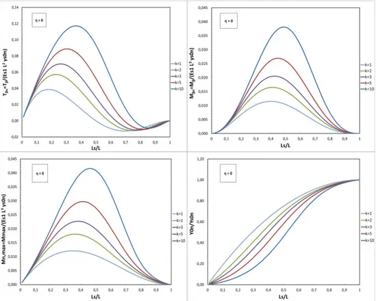
Figure 3-20: Normalised shear force at zn=β, bending moment at zn=β , maximum bending moment and pile head displacement versus Ls/L, for η= and different k values. Free-head condition ... 53
xi
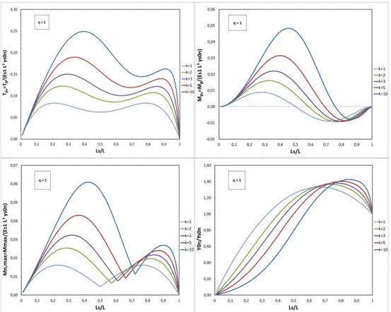
Figure 3-21: Normalised shear force at zn=β, bending moment at zn=β , maximum
bending moment and pile head displacement versus Ls/L, for η= and different k
values. Free-head condition ... 54
Figure 3-22: Normalised shear force at zn=β, bending moment at zn=β , maximum
bending moment and pile head displacement versus Ls/L, for k=2 and different η
values. Unrotated-head condition ... 55
Figure 3-23: Normalised shear force at zn=β, bending moment at zn=β , maximum
bending moment and pile head displacement versus Ls/L for η= and different k
values. Unrotated-head condition ... 56
Figure 3-24: Normalised shear force at zn=β, bending moment at zn=β , maximum
bending moment and pile head displacement versus Ls/L, for η= and different k
values. Unrotated-head condition ... 57
Figure 3-25:Variation of Es with depth for a free-head passive rigid pile in a normal consolidated cohesive soil ... 58
Figure 3-26: Soil profile and pile displacement geometry for a unrotated-head rigid pile in a two-layered cohesive soil ... 59
Figure 3-27: : Normalised shear force with depth for k=2, η=1 and α0=0.5 ... 63
Figure 3-28: : Normalised shear force with depth for k=2 ,η=0 and α0=0.5 ... 64 Figure 3-29: Normalised bending moment with depth for k=2, η=1 and α0=0.5 .. 65
Figure 3-30: Normalised bending moment with depth for k=2, η=0 and α0=0.5 .. 66
Figure 3-31:Soil profile and pile displacement geometry for a unrotated-head passive rigid pile in a normal-consolidated sliding cohesive soil over a firm layer ... 67
xii
Figure 3-32: Normalised shear force with depth for an unrotated pile and for k=2, η=1 and α0=0.5 ... 71 Figure 3-33: Normalised shear force with depth for an unrotated pile and for k=2, η=0 and α0=0.5 ... 72 Figure 3-34: Normalised bending moment with depth for an unrotated pile and for k=2, η=1 and α0=0.5 ... 73 Figure 3-35: Normalised bending moment with depth for an unrotated pile and for k=2, η=0 and α0=0.5 ... 74 Figure 3-36: Normalised shear force at zn=, bending moment at zn= , maximum
bending moment and pile head displacement versus Ls/L, for η=0,k=2 and different
α0 values. Free-head condition ... 78
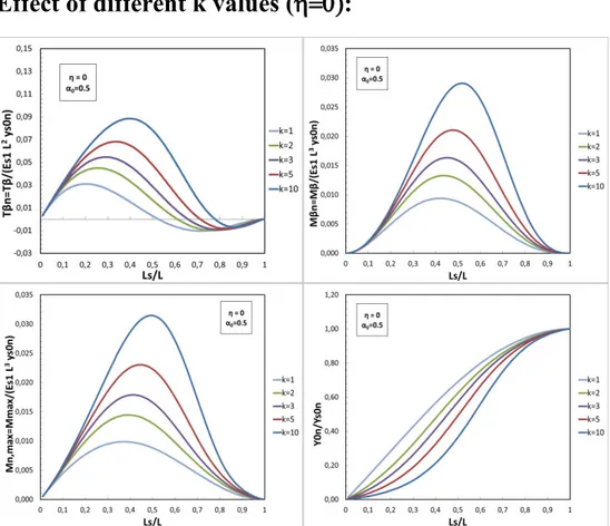
Figure 3-37: Normalised shear force at zn=β, bending moment at zn=β , maximum
bending moment and pile head displacement versus Ls/L, for η=0, α0=0.5 and
different k values. Free-head condition ... 79
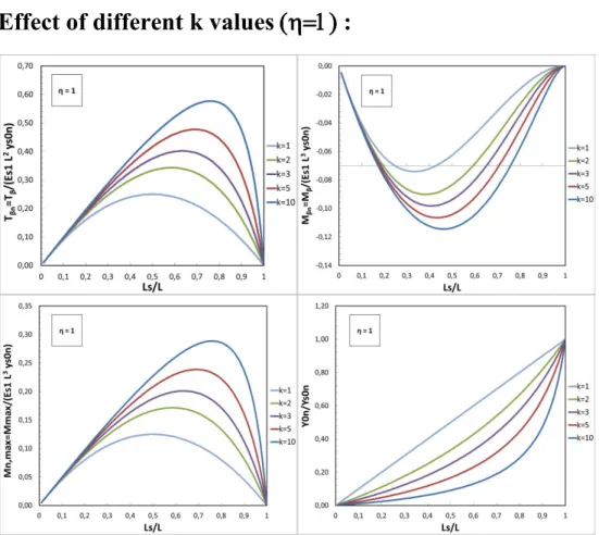
Figure 3-38: Normalised shear force at zn=β, bending moment at zn=β , maximum
bending moment and pile head displacement versus Ls/L, for η=1, α0=0.5 and
different k values. Free-head condition ... 80
Figure 3-39: Normalised shear force at zn=β, bending moment at zn=β , maximum
bending moment and pile head displacement versus Ls/L, for k=2, α0=0.5 and
different η values. Free-head condition ... 81 Figure 3-40: Normalised shear force at zn=β, bending moment at zn=β , maximum
bending moment and pile head displacement versus Ls/L, for η=0, α0=0.5 and
different k values. Unrotated-head condition ... 82
Figure 3-41: Normalised shear force at zn=β, bending moment at zn=β , maximum
bending moment and pile head displacement versus Ls/L, for η=1, α0=0.5 and
xiii
Figure 3-42: Normalised shear force at zn=β, bending moment at zn=β , maximum
bending moment and pile head displacement versus Ls/L, for k=2, α0=0.5 and
different η values. Unrotated-head condition ... 84
Figure 3-43: Normalised shear force at zn=β, bending moment at zn=β , maximum bending moment and pile head displacement versus Ls/L, for k=2, η=0 and different α0 values. Unrotated-head condition ... 85
Figure 3-44: Soil profile and pile displacement geometry for a unrotated-head passive rigid pile in a cohesionless sliding soil over a cohesive firm layer ... 86
Figure 3-45: Variation of Es with depth for a free-head passive rigid pile in a cohesionless sliding soil over a cohesive firm layer ... 87
Figure 3-46: : Normalised shear force with depth for k=2, η=1 ... 91
Figure 3-47: Normalised shear force with depth for k=2, η=0 ... 92
Figure 3-48: Normalised bending moment with depth for k=2, η=1 ... 93
Figure 3-49: Normalised bending moment with depth for k=2, η=1 ... 94
Figure 3-50: Soil profile and pile displacement geometry for a unrotated-head passive rigid pile in a cohesionless sliding soil over a cohesive firm layer ... 95
Figure 3-51: Normalised shear force with depth for k=2, η=1 ... 98
Figure 3-52: Normalised shear force with depth for k=2, η=0 ... 99
Figure 3-53: Normalised bending moment with depth for k=2, η=1 ... 100
Figure 3-54: Normalised bending moment with depth for k=2, η=0 ... 101
Figure 3-55: Normalised shear force at zn=, bending moment at zn= , maximum bending moment and pile head displacement versus Ls/L, for k=2 and different η values. Free-head condition ... 105
xiv
Figure 3-56: Normalised shear force at zn=β, bending moment at zn=β , maximum
bending moment and pile head displacement versus Ls/L, for η =0 and different k
values. Free-head condition ... 106
Figure 3-57: Normalised shear force at zn=β, bending moment at zn=β , maximum
bending moment and pile head displacement versus Ls/L, for η =1 and different k
values. Free-head condition ... 107
Figure 3-58: Normalised shear force at zn=β, bending moment at zn=β , maximum
bending moment and pile head displacement versus Ls/L, for k=2 and different η
values. Unrotated-head condition ... 108
Figure 3-59: Normalised shear force at zn=β, bending moment at zn=β , maximum
bending moment and pile head displacement versus Ls/L, for η =0 and different k
values. Unrotated-head condition ... 109
Figure 3-60: Normalised shear force at zn=β, bending moment at zn=β , maximum
bending moment and pile head displacement versus Ls/L, for η =1 and different k
values. Unrotated-head condition ... 110
Figure 3-61: Soil profile and pile displacement geometry for a free-head passive rigid pile in a three-layered cohesive soil ... 111
Figure 3-62: Variation of Es with depth for a free-head passive rigid pile in a three-layered soil ... 112
Figure 3-63: Normalised shear force with depth for k=2, η=1, λ=0.3 and α0=0.25
... 118
Figure 3-64: Normalised shear force with depth for k=2, η=0, λ=0.3 and α0=0.25
... 119
Figure 3-65: Normalised bending moment with depth for k=2, η=1, λ=0.3 and α0=0.25 ... 120
xv
Figure 3-66: Normalised bending moment with depth for k=2, η=0, λ=0.3 and α0=0.25 ... 121
Figure 3-67: Soil profile and pile displacement geometry for a unrotated-head passive rigid pile in a cohesionless sliding soil over a cohesive firm layer ... 122
Figure 3-68: Normalised shear force with depth for k=2, η=1, λ=0.3 and α0=0.25
... 126
Figure 3-69: Normalised shear force with depth for k=2, η=0, λ=0.3 and α0=0.25 ... 127
Figure 3-70: Normalised bending moment with depth for k=2, η=1, λ=0.3 and α0=0.25 ... 128 Figure 3-71: Normalised bending moment with depth for k=2, η=0, λ=0.3 and α0=0.25 ... 129 Figure 3-72: Normalised shear force at zn=, bending moment at zn= , maximum
bending moment and pile head displacement versus Ls/L, for η=0, α0=0.5,k=2 and
different λ values. Free-head condition ... 133 Figure 3-73: Normalised shear force at zn=, bending moment at zn= , maximum
bending moment and pile head displacement versus Ls/L, for λ =0.3, α0=0.5,k=2
and different η values. Free-head condition ... 134 Figure 3-74: Normalised shear force at zn=, bending moment at zn= , maximum
bending moment and pile head displacement versus Ls/L, for λ =0.3, α0=0.5, η=0
and different k values. Free-head condition ... 135
Figure 3-75: Normalised shear force at zn=, bending moment at zn= , maximum
bending moment and pile head displacement versus Ls/L, for λ =0.3, α0=0.5, η=1
xvi
Figure 3-76: Normalised shear force at zn=, bending moment at zn= , maximum
bending moment and pile head displacement versus Ls/L, for λ =0.3,k =2, η=0 and
different α0 values. Free-head condition ... 137
Figure 3-77: Normalised shear force at zn=, bending moment at zn= , maximum bending moment and pile head displacement versus Ls/L, for λ =0.3, α0=0.5, η=0 and different k values. Unrotated-head condition ... 138
Figure 3-78: Normalised shear force at zn=, bending moment at zn= , maximum bending moment and pile head displacement versus Ls/L, for λ =0.3, α0=0.5, η=1 and different k values. Unrotated-head condition ... 139
Figure 3-79: Normalised shear force at zn=, bending moment at zn= , maximum bending moment and pile head displacement versus Ls/L, for λ =0.3, α0=0.5, k=2 and different η values. Unrotated-head condition ... 140
Figure 3-80: Normalised shear force at zn=, bending moment at zn= , maximum bending moment and pile head displacement versus Ls/L, for η=0, α0=0.5, k=2 and different λ values. Unrotated-head condition ... 141
Figure 3-81: Normalised shear force at zn=, bending moment at zn= , maximum bending moment and pile head displacement versus Ls/L, for λ=0.3,k =2, η=0 and different α0 values. Unrotated-head condition ... 142
Figure 3-82: Soil profile and pile displacement geometry for a rigid pile in cohesionless soil ... 143
Figure 3-83: Normalised shear force with depth for η=1 ... 147
Figure 3-84: Normalised shear force with depth for η=0 ... 148
Figure 3-85: Normalised bending moment with depth for η=1 ... 149
xvii
Figure 3-87: Soil profile and pile displacement geometry for a unrotated-head
rigid pile in a cohesionless soil ... 151
Figure 3-88: Normalised shear force with depth for η=1 ... 154
Figure 3-89: Normalised shear force with depth for η=0 ... 155
Figure 3-90: Normalised bending moment with depth for η=1 ... 156
Figure 3-91: Normalised bending moment with depth for η=0 ... 157
Figure 3-92: Normalised shear force at zn=, bending moment at zn= , maximum bending moment and pile head displacement versus Ls/L, for different η values and free-head condition ... 160
Figure 3-93: Normalised shear force at zn=β, bending moment at zn=β , maximum bending moment and pile head displacement versus Ls/L, for different η values and unrotated-head condition ... 161
Figure 4-1: Variation of Np with s/D for a = 0, 0.25, 0.5, 0.75 and 1 as proposed by Georgiadis K. et al. [45] ... 169
Figure 4-2: Pile failure modes: (a) failure mechanism A; (b) failure mechanism B; (c) failure mechanism C [23], [28], [46] ... 172
Figure 4-3: Soil profile and pile displacement geometry ... 174
Figure 4-4:Distribution of the soil movement: a) generic distribution; b) inverse triangular variation with depth h=0; c)uniform distribution with depth h=1 .... 175
Figure 4-5:(a) Rigid pile deflection; (b) Variation of Es with depth; (c) Variation of pu with depth ... 176
Figure 4-6: First yielding points and corresponding first yielding case ... 181
xviii
Figure 4-8: Example of first yielding non-dimensional displacement Ys0n diagram over Ls/L ... 186
Figure 4-9: Soil pressure distribution for the different cases C1, C2 and C3. The dashed line represents the limit soil resistance distribution while the blue line the pile-soil reaction ... 190
Figure 4-10: Soil pressure distribution for the different cases B1-L1, B1-L2, B2-L1 and B2-L2. The dashed line represents the limit soil resistance distribution while the continue line the pile-soil reaction ... 191
Figure 4-11: Dimensionless shear force induced in a two-layered cohesive soil at sliding depth as a function of the normalized sliding depth at the ultimate state for soil sliding with both a triangular and uniform distribution over depth (fixed L0/L=0.35, k0=2/9, k=2.0, eta=1. Only values for Ls>L0 are shown)and the
solutions as presented by Viggiani [23]. ... 193
Figure 4-12: Design curves for piles in two layered cohesive soil; L0/L=0.35,
k0=2/9, k=2.0, eta=1; non-dimensional shear force Tn over and ysn. Dotted line
represents the limit elastic solutions and the red one the ultimate pile resistance197
Figure 4-13: Design curves for piles in two layered cohesive soil; L0/L=0.35,
k0=2/9, k=2.0, eta=1; non-dimensional shear force Tn over and y0n. Dot line
represents the limit elastic solutions and the red one the ultimate pile resistance198
Figure 4-14: Design curves for piles in two layered cohesive soil; L0/L=0.35,
k0=2/9, k=2.0, eta=1; non-dimensional shear force Tn over and Mn. Dot line
represents the limit elastic solutions and the red one the ultimate pile resistance199
Figure 4-15: Design curves for piles in two layered cohesive soil; L0/L=0.35,
k0=2/9, k=2.0, eta=0; non-dimensional shear force Tnover β and Y0n. To be
noticed the negative values of Tn for ys>0.57. Dot line represents the limit elastic
xix
Figure 4-16: Design curves for piles in two layered cohesive soil; L0/L=0.35,
k0=2/9, k=2.0, eta=0; non-dimensional shear force Tn over β and ysn. Dot line
represents the limit elastic solutions and the red one the ultimate pile resistance201
Figure 4-17: Design curves for piles in three layered cohesive soil; L0/L=0.35,
k0=2/9, k=2.0, eta=0; non-dimensional shear force Tnover β and Mn. Dot line
represents the limit elastic solutions and the red one the ultimate pile resistance202
Figure 4-18: Soil displacement distribution, pile displacement geometry,
distributions of the subgrade reaction modulus and of the ultimate soil pressure for a rigid pile in cohesionless soil ... 207
Figure 4-19: Identified yielded region and their nomenclature ... 212
Figure 4-20: Soil pressure distribution for the different cases C1, C2 and C3. The dashed line represents the limit soil resistance distribution while the continue one the pile-soil profile ... 213
Figure 4-21: Soil pressure distribution for the different cases A1, A2 and A3. The dashed line represents the limit soil resistance distribution while the continue one the pile-soil reaction ... 214
Figure 4-22: Soil pressure distribution for the different cases B1 B2-L2. The dashed line represents the limit soil resistance distribution while the continue line the pile-soil reaction ... 216
Figure 4-23: Dimensionless shear force Tm=T/(mL 2
) offered by a pile in a non-cohesive soil at the sliding depth for different configurations: soil sliding with a triangular distribution over depth, soil sliding with a uniform distribution over depth ... 217
Figure 4-24: Curves of normalised shear force Tm over Ls/L for =1. Numbers
indicates the external normalised soil displacement ys0*m/n. Dashed line
xx
Figure 4-25: Curves of normalised shear force Tm over Ls/L for = 0. Numbers
indicates the external normalised soil displacement ys0*m/n. Dashed line
represents the limit elastic solutions ... 221
Figure 4-26: Curves of normalised shear force Tm over Ls/L for =1. Numbers
indicates the external normalised pile head displacement y0*m/n. Dashed line represents the limit elastic solutions ... 222
Figure 4-27: Curves of normalised shear force Tm over Ls/L for =0. Numbers
indicates the external normalised pile head displacement y0*m/n. Dashed line represents the limit elastic solutions ... 223
Figure 4-28: Curves of normalised shear force Tm over Ls/L for =1. Numbers
indicates the normalised maximum bending moment Mmax/(mL 3
). Dashed line represents the limit elastic solutions ... 224
Figure 4-29: Curves of normalised shear force Tm over Ls/L for =0. Numbers
indicates the normalised maximum bending moment Mmax/(mL 3
). Dashed line represents the limit elastic solutions ... 225
Figure 5-1: Soil profile used in the analysis ... 228
Figure 5-2: Failure mechanisms for non-yielding piles: (a) failure mechanism A; (b) failure mechanism B; (c) failure mechanism C ... 233
Figure 5-3: Failure mechanisms for yielding piles: (a) failure mechanism B1; (b) failure mechanism BY; (c) failure mechanism B2 ... 237
Figure 5-4: Dimensionless resistance offered by non-yielding piles at the depth of sliding (a) shear (b) bending moment ... 238
Figure 5-5:Dimensionless shear offered by yielding piles at the depth of sliding; (a) X=1; (b) X= 0.5 ... 240
xxi
Figure 5-6: Dimensionless bending moment offered by yielding piles at the depth of
sliding; (a) X=1; (b) X= 0.5 ... 240
Figure 6-1: Schematic cross section of a pile reinforced slope ... 242
Figure 6-2: Theoretical forces due to a pile row to include in slope stability analyses ... 243
Figure 6-3:Cross section of slope stabilizing pile [66] ... 249
Figure 6-4: Forces acting on a typical slice [66] ... 250
Figure 6-5: Effect of variation in internal friction angle on Rp[67] ... 251
Figure 6-6: Optimisation of pile spacing and pile row location[66] ... 252
Figure 6-7: Method of slices using two rows of drilled shafts [70] ... 253
Figure 6-8: Shaft force versus shaft location for different (S, D) combinations using one row of drilled shafts [70] ... 254
Figure 6-9: Schematic illustration of the two steps of the decoupled methodology: (a) limit equilibrium slope stability analysis to compute the additional required resistance force RF; (b) estimate pile configuration capable of providing the required RF at prescribed displacement [21] ... 255
Figure 6-10: Geometry of a pile-reinforced slope [43] ... 257
Figure 6-11: Slope geometry and pile contribution according to Jeong et al.[54] ... 258
Figure 6-12: Forces acting on a pile-stabilised slope[71] ... 260
xxii
TABLE OF CONTENTS
ABSTRACT ... v LIST OF TABLES ... vi LIST OF FIGURES ... ix TABLE OF CONTENTS ... xxii NOTATION ... xxv 1. Introduction ... 1 2. Analysis methods of passive piles ... 3 2.1. Pile-supported embankments ... 4 2.2. Piles adjacent to deep excavation... 6 2.3. Passive piles to increase slope stability ... 8
2.3.1. Numerical methods ... 8 2.3.2. Analytical methods ... 9 2.3.3. Pressure-based methods ... 10 2.3.4. Displacement-based methods ... 11
3. Passive pile in a linear elastic soil: a displacement-based model for passive pile in a linear elastic soil ... 15 3.1. Overview of the Winkler model... 17 3.2. Problem definition and model hypotheses ... 20 3.3. Estimation of elastic soil parameters ... 28 3.4. Elastic solutions for a passive rigid pile in a two-layered cohesive soil with a
constant subgrade reaction modulus ... 31
3.4.1. Estimation of elastic soil parameters ... 32 3.4.2. Elastic solutions for the free-head condition ... 33 3.4.3. Elastic solutions for the unrotated-head condition ... 41 3.4.4. Parametric analysis ... 49
3.5. Elastic solutions for a passive rigid pile in a two-layered soil with subgrade modulus varying with depth ... 58
3.5.1. Free-head condition ... 58 3.5.2. Unrotated head condition ... 67 3.5.3. Parametric analysis ... 75
3.6. Elastic solutions for a passive rigid pile in a two-layered profile with subgrade modulus linearly increasing with depth ... 86
xxiii
3.6.1. Free-head condition ... 86 3.6.2. Unrotated head condition ... 95 3.6.3. Parametric analysis ... 102
3.7. Elastic solutions for a passive rigid pile in a three-layered soil ... 111
3.7.1. Free-head condition ... 111 3.7.2. Elastic solutions for unrotated-head condition ... 122 3.7.3. Parametric analysis ... 130
3.8. Elastic solutions for a passive rigid pile on a soil with Es linearly increasing with depth ... 143
3.8.1. Free-head condition ... 143 3.8.2. Elastic solutions for an unrotated-head passive rigid pile on a cohesionless soil
151
3.8.3. Parametric analysis ... 158
4. Elasto-plastic analysis of passive rigid piles in cohesive soils ... 162 4.1. Limiting soil resistance pu ... 164 4.1.1. Limiting soil resistance a single passive pile ... 164 4.1.2. Limiting soil resistance for a row of piles ... 166
4.2. Modes of failure for a passive pile ... 170 4.3. Elasto-plastic analysis of passive rigid piles in cohesive soils ... 174
4.3.1. Soil profile and geometry of the problem ... 174 4.3.2. Constitutive model and ultimate soil resistance pu ... 176 4.3.3. Method of analysis ... 179 4.3.4. First yielding cases and threshold soil displacements ... 181 4.3.5. Iterative numerical procedure and cases ... 187 4.3.6. Failure modes... 189 4.3.7. Design charts ... 194 4.3.8. Results and discussion ... 203
4.4. Elasto-plastic analysis of passive rigid piles in a homogeneous non-cohesive soil ... 206
4.4.1. Geometry, constitutive model and ultimate soil resistance pu ... 207 4.4.2. Method of analysis, first yielding cases and threshold soil displacements ... 210 4.4.3. Failure modes... 213 4.4.4. Design charts ... 218 4.4.5. Results and discussion ... 226
5. Lateral resistance of passive piles in a double-layered non-cohesive soil .... 227 5.1. Geometry ... 227 5.2. Limiting soil pressure ... 229 5.3. Failure modes for non-yielding piles ... 230 5.4. Failure modes for yielding piles... 234 5.5. Results and discussion ... 238
xxiv 5.6. Final considerations ... 241 6. Stability analysis of slopes reinforced with piles ... 242 6.1. Stability analysis of a pile-reinforced slope ... 242
6.1.1. Numerical methods ... 244 6.1.2. Limit analysis... 246 6.1.3. Limit Equilibrium methods ... 247
6.2. Discussion and application of the proposed method ... 261
6.2.1. Stable slopes ... 262 6.2.2. Unstable slope ... 266
7. Conclusion and Recommendations ... 269 7.1. Summary ... 269 7.2. Future Researches ... 271 REFERENCES ... 272 APPENDICES ... 279 APPENDIX A: Cases for the elasto-plastic analysis of passive rigid piles in cohesive soils ... 280 APPENDIX B: Cases for the elasto-plastic analysis of passive rigid piles in a
xxv
NOTATION
N = normal force T = shear force M = bending moment D = pile diameterFd = total of the disturbing actions along a slip surface Fr = total of the resisting actions along a slip surface
MR = total of the resisting bending moments along a slip surface Md = total of the disturbing bending moments along a slip surface SF = factor of safety of a unreinforced slope
SFT = factor of safety of a pile-reinforced slope SFtarget = target factor of safety for a pile-reinforced slope RF = slope stabilising contribution provided by the piles Np = ultimate undrained lateral bearing capacity factor s = centre-to-centre pile spacing in a row
d = clear spacing between the piles in a row = pile-soil adhesion factor
s1 = critical pile spacing
Np1 = ultimate undrained lateral bearing capacity factor py = yielding soil-pile pressure [FL-2]
p(z) = elastic force per unit length of the pile at the depth z [FL-1] pu = ultimate force per unit length of the pile [FL-1]
Kp = Rankine passive pressure coefficient φ’ = internal friction angle of the soil c’ = effective cohesion of the soil
φR = reduced internal friction angle of the soil cR = reduced cohesion of the soil
Su = undrained shear strength of soil �′ = initial vertical effective stress = total unit weight of the soil
’ = effective soil unit weight of the soil h = load transfer reduction factor
xxvi kh = coefficient of subgrade reaction of a soil mass [FL−3 ]
Es = subgrade reaction modulus or elastic spring modulus [FL−2 ] L = pile length
Ls, L1 = sliding surface depth (βL) L0 = first layer thickness (λL) L2 = firm layer thickness
β = ratio between sliding depth and pile length Ls/L = ratio between first layer thickness and pile length L0/L Ep = Young’s modulus of the pile
Jp = Moment of inertia of the pile section I = characteristic pile length [L]
z,zn = depth and the normalised depth z/L, respectively yp(z) = pile deflection at the depth z
y0 = pile head’s deflection at ground level
y0n = normalised pile head’s deflection at ground level Y0/L ω = pile rotation angle
M0 = bending moment on pile head for the unrotated head fixity condition M0n = normalised bending moment on pile head for the unrotated head fixity
condition T = shear force
Tn,Tm = normalised shear force M = bending moment
Mn = normalised bending moment My = yielding moment of the pile section ys(z) = soil movement at the depth z
ys0 = soil free-field movement at ground surface
ys0 = normalised soil free-field movement at ground surface Ys0 /L = angle of linear variation of the free-field soil movement = ratio between soil displacement at ground level and at Ls Y(z) = relative soil-pile displacement at a generic depth of z ∆ = relative soil-pile displacement at ground level
∆ = normalised relative soil-pile displacement at ground level ∆ � = relative soil-pile tangent of rotation angle
xxvii k = ratio between Es or pu of stable and unstable soils
α0 = ratio between modulus of subgrade reaction at ground level and at Ls or L0 when linearly varying with depth
k0 = ratio between pu at ground surface and stable and at z=L0 m = gradient of the ultimate force per unit length of the pile (FL-2)
m1,m2 = gradient of pu for unstable and stable layer X = ratio of gradients of pu (
X = m
1/m
2)n = gradient of the horizontal subgrade reaction modulus (FL-3) Ny = Proportionality constants in the elastic solutions
Nt = Proportionality constants in the elastic solutions NΔy = Proportionality constants in the elastic solutions NΔt = Proportionality constants in the elastic solutions NM = Proportionality constants in the elastic solutions D = Proportionality constants in the elastic solutions
a = coefficients of a six order governing equations for failure mode B, B1, BY and B2
1
1. Introduction
When subjected to a lateral force due to the horizontal movements of the surrounding soil, piles are defined as passive piles, in opposition to active piles, i.e. being part of piled walls, subjected to applied forces. Obviously, both kinds of situations are governed by the same series of parameters as the deformability of the pile and the soil and the ultimate soil resistance, all governed by the interaction soil-pile.
Anyway, active piles transmit lateral loads to the soil due to a horizontal load applied on it, being the horizontal soil movements the consequence of their action. They are frequently used for supporting axial and lateral loads for different structures, cases in which the horizontal loads governs the design of the piles. The problem of active piles either in clay or sand has already been treated by several authors (Broms [1], Matlock and Reese [2], Zhang L. [3]), by using different approaches.
On the contrary, piles which are subjected to lateral loading along their length caused by horizontal movements of the surrounding soil are instead defined as passive piles. Passive load on the piles may occur every time changes in the surrounding soil stress state provoke a movement in the soil mass, for example those installed close to embankments, tunnels or earthworks. Typical cases are piles solicited by the installation of adjacent others or crossing liquefying layers subjected to earthquakes.
Another common example is the use of shaft in unstable slopes to prevent or reduce the occurrence of slope failures. The use of piles to stabilise active landslides or to prevent future events has been successfully applied in the past, due to the easy installation in slopes which does not disturb or compromise the equilibrium of the land.
However, there remain uncertainties on the design of passive piles, and an agreement on how to model passive piles has still to be reached, due to the complex phenomena ruling the soil-pile interaction and the several factors affecting it.
2 The presented research work has the primary goal of developing a reliable and representative design method that accounts for the effect of the soil and pile properties on the performance of passive piles based on the soil-pile interaction. The method results to be capable to analysis and design passive piles, estimating the pile reaction as a function of the external soil displacement acting on it as well as predicting the complete pile deflection and stress state.
In particular, several different soil stratigraphy and pile boundary conditions are analysed and relative elastic or elasto-plastic solutions of the soil-pile system are developed. The proposed design approach was also compiled into a computer program for the analysis of pile-soil system.
In addition, examples of practical design charts are also shown as results of the implemented methodology.
3
2. Analysis methods of passive piles
The definition of active piles refers to a pile subjected to an external horizontal force and, eventually, a bending moment applied on its head. On the other hand, if subjected to a soil movement, piles are known as passive piles (Figure 2-1).
Figure 2-1:Schematic sections of : a) Active pile with length L, diameter D. b) Passive pile embedded in a surrounding sliding soil
Driven or drilled piles work as passive piles whenever they are installed to prevent or at least reduce the likelihood of slope failure or are subjected to a lateral force due to the horizontal movements of the surrounding soil if changes in the stress state provoke a movement in the soil mass.
Soil movement is also encountered in practice when piles are placed in an unstable slope, landslides, adjacent to deep excavation, tunnel operation, marginally stable riverbank with high fluctuating water level and also in piles supporting bridge abutment adjacent to approach embankments.
This chapter attempts to present an overview mainly for single pile in different topics: pile-supported embankment, piles adjacent to deep excavation, pile
4 subjected to horizontal soil movement as used for slope stabilisation. It aims to be only an overview and brief description of the contributions given by various researchers and to present the discussion mainly to emphasise the significance of past researches on passive piles used as stabilising system.
2.1. Pile-supported embankments
The consolidation of embankments on clay can produce significant vertical and horizontal movements of the adjacent soil. Piles supporting bridge abutments might then be axially and laterally loaded by these soil movements. The assessment of the resulting axial force and movement, bending moment and lateral deflection developed in the piles are then fundamental for the design of the piles. Figure 2-2 shows a schematic section through such a structure, illustrating the forms of interaction which tend to increase lateral structural loading and displacement, and hence may result in unserviceable behaviour of the abutment or bridge deck.
Figure 2-2: Schematic section through a full-height piled bridge abutment constructed on soft clay [4]
5 De Beer & Wallays [5] proposed a simple semi-empirical method to estimate the maximum bending moment for piles subjected to asymmetrical surcharges. They assumed that a constant lateral pressure distribution acted on the pile in the soft layer and assessed the magnitude of this lateral pressure as a function of the total vertical lithostatic pressure, friction angle and the slope of a fictitious embankment of material. They suggested that the lateral loading was caused by horizontal consolidation and creep, involving that their method was primarily intended to design piles in the long term. Otherwise, the method cannot be used to calculate the variation of bending moment with depth along the pile. Therefore, they conservatively recommended that the piles should be reinforced over their whole length to carry the maximum calculated bending moment. After calibrating the method against a few case studies, they demonstrated that the method is only suitable if a large margin of safety is provided against the overall instability of the soil mass.
The effects of vertical drains in the clay layer within embankments was investigated by Ellis [6] through a series of geotechnical centrifuge tests of full-height piled bridge abutments examining the effect of soft clay layer depth and the rate of embankment construction. The results confirmed the existence of established interaction effects due to lateral displacement of clay past piles.
Following this, Ellis and Springman [4] presented an accompanying series of plane strain finite element analyses for the same series of geotechnical centrifuge tests to study the soil-structure interaction effects. Although some aspects of the structure do not conform to a plane strain analysis (most notably the piles), success of the method is illustrated by good comparison with the centrifuge test results.
For piles to support a retaining wall, the recommendations of Terzaghi et al. [7] embodied in charts, are based on the use of the equivalent-fluid method and show the importance of the selection of an appropriate material for the backfill. A comparison of values from theory with values from the charts shows that the charts are close to those from Rankine’s theory for active earth pressure. Therefore, the assumption is implicit in the Terzaghi charts that the wall is capable of some
6 movement without distress if the pressures from the backfill were greater than the chart values.
Finally, it is worth to be noticed the work made by Poulos [8], who reviewed some available design methods of piles through embankment and presented comparison between these methods for maximum bending moment in the piles, lateral pile head deflection, maximum axial force in pile and axial pile head settlement. Some of the methods being reviewed are the method of De Beer and Wallays [9], an approach used by a road authority in Australia, a simplified analysis of pile downdrag and design charts developed from boundary element analyses of pile-soil interaction. It is interesting that the author concludes that none of the previously available methods appears able to provide a consistent means of estimating the lateral response of piled embankment.
2.2. Piles adjacent to deep excavation
In dense urban environment where buildings are closely spaced, deep excavation for basement construction and other underground facilities is unavoidable. These deep excavations would cause lateral soil movement behind the excavation, which would in turn induce lateral loading on adjacent pile foundations and consequently additional bending moment and deflection.
For example, Finno et al. [10] reported the analyses of performance of groups of piles located adjacent to a 50-ft-deep tieback excavation. Evaluation of effects of movements on the adjacent piles was then carried out using a plane strain finite element code. However, accuracy of the approach could not be clearly verified due to less certainty with the selection of soil parameters, especially the soil’s modulus because of the lack of detailed laboratory or in situ testing.The uncertainty of modelling the equivalent bending stiffness of the pile group in plane strain resulted in lower and upper bound solution.
7 Poulos & Chen [11] did a two stage analysis by use of the finite-element method and the boundary-element method to analyse the response of piles due to unsupported excavation-induced lateral soil movement in clay. Initially, a plane strain finite element method was used to simulate the excavation procedure and to generate free-field soil movements, that is the soil movement that would occur. These generated soil movements are then used as input into a boundary element method to analyse the pile’s response.
On the contrary, Goh et al. [12] presented the results of an actual full-scale instrumented study carried out to examine the behaviour of an existing pile due to nearby excavation of a 16m deep excavation with an in-soil inclinometer installed about 6m away . The instrumented existing pile was discretized into a finite number of discrete (linear elastic) beam elements. The interaction between the soil and the pile is modelled by a series of non-linear horizontal springs represented by a hyperbolic equation.
Recent efforts in centrifuge modelling of passive piles adjacent to unsupported excavation were done by Leung et al. [13] who presented the results of centrifuge tests of a single pile behind a stable and failed wall of a deep excavation in dense sand. The research also investigates the influence of head fixity and shows that behind the stable wall, the pile head deflection and maximum bending moment for the free-headed pile decrease exponentially with increasing distance from the wall. Subsequently, he extended the centrifuge test to pile groups, incorporating the effects of interaction factors between the piles with different head fixities [14]. Further investigation was done for single pile behind stable wall [15] and unstable wall [16] in clay. It is concluded that calculated pile response is in good agreement with the measured data if correct shear strength obtained from post-excavation was used in numerical analysis. The numerical analysis was based on a simplified model and was used to back-analysed the responses of single pile subjected to lateral soil movements in clay. In this model, the pile is modelled as a series of linear elastic beam elements and the soil is idealised using the modulus of subgrade reaction. This numerical method has been also adopted successfully to back-analyse the centrifuge model tests on a single pile in sand.
8
2.3. Passive piles to increase slope stability
At present, simplified methods based on crude assumptions are used to design the driven or drilled piles needed to stabilise the slopes of embankments or to reduce the potential for landslides from one season to another. The major challenge lies in the evaluation of lateral loads (pressure) acting on the piles/pile groups by the moving soil and in the development of a representative model for the soil-pile interaction above and below the failure surface, both required to reflect and describe the actual distribution of the soil-pile pressure along the length of the pile. The different mechanisms of failure and factors can be considered in the evaluation of the resistance contribution a pile can transmit implicate a distinction between two groups of methods used to describe soil-pile interaction: analytical methods, like pressure or displacement-based ones, and numerical methods, such as finite elements and finite differences. Nevertheless, it is important to highlight that a similarity of the applicability of method of analysis by using plane strain finite element method, subgrade reaction or elastic continuum formulation is that a specified free-field soil movement have to be inputted in the numerical method to analyse the response of the piles in terms of deflection.
2.3.1. Numerical methods
Over the last few years, the progress in computing and software power led to a wide application of the finite-element (FE) and finite differences (FD) methods, which provide the ability to model complex three-dimensional geometries and to run coupled analysis of soil-structure interaction such as pile group effects (Chow [17]; Cai and Ugai [18]; Won et al.[19]; Wei and Cheng [20];) as 2D analysis do not capture some aspect of the problem as soil arching. However, the applications of numerical methods in three dimensions are rather unattractive for practitioners as they are complex, computationally expensive and time-consuming.
Among all, Chow [17] presented a numerical approach in which the piles are modelled using beam elements and the surrounding soil using an average modulus
9 of subgrade reaction. The theory of elasticity is therefore used to simulate the soil-pile-soil interaction while the sliding soil movement profile is assumed according to field measurements. The same method has been used later by Cai and Ugai [18] for the same scope.
More recently, Kourkoulis et al. 2011 [21], [22] developed a hybrid methodology for the design of slope-stabilizing piles aimed at reducing the amount of computational effort usually associated with 3D soil-structure interaction analyses. This method involves all the steps for evaluating the required lateral resisting force per unit length of the slope, needed to increase the safety factor to the desired value by using the results of a conventional slope stability analysis, and for estimating the pile configuration that offers the required force for a prescribed deformation level using a 3D finite element analysis. This approach computes the lateral capacity of the piles by numerically three-dimensionally simulating only a limited region of soil around the piles and imposing a uniform displacement profile into the model boundary.
2.3.2. Analytical methods
The analytical methods used for the analysis of passive piles can generally be classified into two different types: pressure-based methods and displacement-based methods.
The pressure-based methods (Broms [1]; Viggiani[23]; Randolph and Houlsby, [24]; Ito and Matsui [25]) are centred on the analysis of passive piles that are subjected to the ultimate lateral soil pressure. The most notable limitation of pressure-based methods is that they apply to the ultimate state only (providing ultimate soil-pile pressure) and do not give any indication of the development of pile resistance with soil movement (mobilised soil-pile pressure). Therefore, their application should be limited to already stable soil configurations, in which piles are called to give a contribution to reach a mandatory higher factor of safety. In displacement-based methods (Poulos [26]; Lee et al. [27]), the lateral soil movement above the failure surface is used as an input to evaluate the associated
10 lateral response of the pile. These methods are superior to the pressure-based ones as they can provide the mobilised pile resistance by considering the soil external movement as the input of the calculation. In addition, they reflect the true mechanism of soil-pile interaction. For this reason, this kind of methods better fit with analysis of slopes where a soil movements are already acting: the free-field soil movements that can be evaluated by monitoring the landslide or by modelling the slope behaviour can be used as an input for the calculation of the piles response, making possible to optimise their design according to the admissible displacements of the retaining piles wall or of the ground.
Due to this advantages, the analytical displacement-based approach has been chosen for the development of the method object of the present dissertation. However, in the following paragraph a list of the more interesting methods is given in order to provide a review of the methods available in literature
2.3.3. Pressure-based methods
Analysing different soil-pile failure modes with depth, Broms [1] suggested the several equations to calculate the ultimate soil-pile pressure pu for a single pile both in sand, as a function of the Rankine passive pressure coefficient Kp, and in cohesive soils, as function of the undrained shear strength Su and of a bearing capacity factor Np varying with depth.
Viggiani [23] proposed a simplified method in which the maximum shear force provided by a single unrestrained pile is derived assuming that soil movements are great enough to fully mobilise the limiting soil pressure above and/or below the sliding surface. With this assumption, Viggiani derived dimensionless solutions for the ultimate lateral resistance of a pile in a two-layer purely cohesive soil profile. These solutions provide the pile shear force at the slip surface and the maximum pile bending moment as a function of the pile length and the ultimate soil-pile pressure pu in stable and unstable soil layers. With this assumption, six failure modes were analysed and dimensionless solutions for shear force and maximum bending moment are derived for each potential failure mechanism (Chmoulian [28]). The solution of Viggiani is applicable only to soil in undrained condition
11 with an ultimate lateral pressure constant with depth in the stable and unstable layer.
Among all, Guo [29] proposed pressure-based pile–soil models and developed their associated solutions to capture response of rigid piles subjected to soil movement. The impact of soil movement was schematized as a fixed distributed loading over a sliding depth, and load transfer model was adopted to mimic the pile–soil interaction. The soil is modelled according to a Winkler approach with an assumption of a constant subgrade reaction modulus with depth. The solutions are presented in explicit expressions and can be readily obtained. It should be noticed that, along the length subjected to the soil displacement, both the fixed distributed external loading and the reaction pressure due to the soil-pile interaction are acting on the pile at the same time.
2.3.4. Displacement-based methods
In displacement-based methods (Poulos, [26]; Lee et al., [27]), the lateral soil movement above the failure surface is used as an input to evaluate the associated lateral response of the pile. The superiority of these methods over pressure-based methods is that they can provide mobilised pile resistance by soil movement. In addition, they reflect the true mechanism of soil-pile interaction.
Poulos [26] in particular presented a method of analysis of a row of passive piles practically as improvement of the solutions already provided by Viggiani [23], aiming to describe the full soil-pile interaction and not only the ultimate lateral state. For this reason, the pile is modelled as an elastic beam and the soil as an elastic continuum and the calculation carried out by using a finite-difference method (Figure 2-3), so that the model can evaluate the maximum shear force that each pile can provide based on an assumed free-field soil movement input and also compute the associated lateral response of the pile. Poulos assumes that a large volume of soil (the upper portion) moves downslope as a block over a relatively thin zone undergoing intense shearing in the “drag” zone (Figure 2-4). It is assumed an elasto-plastic model for both the pile and the soil: the soil close to the pile interface can undergo elastic strains until the limit pressure is reached (both the
12 elastic modulus and the limit pressure of the soil are assumed as varying along pile length).
Figure 2-3: Model for piles in soil undergoing lateral movement [26]
It should be noticed that, while the pile and soil strength and stiffness properties are taken into account to obtain the soil-pile pressure, the group effects, namely pile spacing, are not considered in the analysis of the soil-pile interaction.
Figure 2-4: Free-field soil movement [26]
The analysis revealed the following failure modes, basically the same found by Viggiani [23]:
13 -The “flow mode” (or Mode C), when the depth of the failure surface is shallow and the sliding soil mass becomes plastic and flows around the pile (see Figure 2-5a). In this case, the pile deflection is considerably less than the soil movement. -The “intermediate mode” (or Mode B), when the depth of the failure surface is relatively deep and the soil strength along the pile length in both unstable and stable layers is fully mobilised (see Figure 2-5b). In this mode, the pile deflection at the upper portion exceeds the soil movement and a resisting force is applied from downslope to this upper portion of the pile.
-The “short pile mode” – when the pile length embedded in stable soil is shallow and the pile will experience excessive displacement due to soil failure in the stable layer (Figure 2-5c).
-The “long pile failure” – when the maximum bending moment of the pile reaches the yields moment (the plastic moment) of the pile section and the pile structural failure takes place (Mmax = My).This mechanism can be associated with any of the others, even if experience suggests that it is most likely to occur with the intermediate mode.
What it is worth to be highlighted is that the maximum shear force in the pile is always developed at the level of the slip surface; its maximum value occurs when the soil slide depth is about 0.5-0.6 times the pile length. Moreover, For practical uses, the author endorsed the flow mode as it creates the least damage from soil movement on the pile. Otherwise, as maximum shear forces and bending moments are developed under the intermediate mode, slope stabilising piles should be designed so that this mode of behaviour occurs.
14
Figure 2-5: Pile behaviour characteristics for various modes with the hypothesis of constant soil movement in the slide zone, no “drag” zone, pile length of 15m and diameter
15
3. Passive pile in a linear elastic soil: a
displacement-based model for passive
pile in a linear elastic soil
Elastic solutions for laterally loaded piles are utilised successfully to predict the behaviour of passive piles. Recent studies suggest that the response of rigid passive piles is dominated by elastic pile–soil interaction [30]. They reveal that about one-third of limiting pressure on passive piles is induced by an elastic interaction. According to Chen and Poulos [31], relatively small soil movements, generally of the order of 5% of the pile diameter, are sufficient to fully mobilise the pile response obtained by mean of an elastic soil behaviour.
For this reason, the present work proposes a displacement-based model for the design of stabilising piles and develops their associated elastic solutions targeting the response in terms of shear force and bending moment along a rigid pile subjected to horizontal soil movement. Therefore, in comparison with available solutions for the ultimate state, the research aims at the development of a general framework focusing on the response of a pile to free-field soil movements, based on purely elastic soil behaviour and considering any stage of ground movement. The only static response is deemed. The analysis is designed to be subsequently improved to incorporate the nonlinear stress-strain relationships of soils and ultimate states, as described in next chapters.
More in particular, the analysing method considers a single rigid pile embedded in a sliding mass. Avoiding an initial assumption on the soil impact pressure on the shafts, the lateral displacement of the moving soil interesting the shaft is used as an input to evaluate the associated lateral deflection and strain state of the pile, according to the sliding depth and the ground and pile strengths. The method can consider a general linear free field soil movement with extreme cases represented by a uniform and an inverse triangular variation with depth. In light of a Winkler model [32], the pile-soil reaction is given by the coefficient of subgrade Es and is represented by force per unit length. The solutions of the equilibrium equations
16 between the soil-pile pressures calculated both above and below the sliding surface are developed in explicit expressions for calculating bending moments, shear forces and deflection.
Different soil stratigraphies and pile boundary conditions are analysed to encompass the more common design configurations, as the presented result seems to be suitable for being implemented in traditional Limit Equilibrium Methods or more in general in any decoupled approach method, whenever the analysed slope presents an active landslide.
17
3.1. Overview of the Winkler model
Research on analysis of passive piles started more than five decades ago. As a consequence of such sustained research, several analysis methods have been developed and can be used for the design (an account of the salient available methods has been provided in chapter 2). While solutions for the ultimate lateral resistance of a pile do not give any indication of the development of pile resistance with soil movement and take into account only the limiting soil pressure, in a displacement based analysis the soil strain and stress levels are linked to the relative soil-pile displacement through an appropriate constitutive model.
In the presented research work, the governing equations for the deflection of passive rigid piles are obtained by using a beam-on-elastic-foundation (or Winkler) approach. It illustrates how simple idealisations of the pile-soil interaction can be used to derive the equations for layered, elastic foundations and to develop the analytical equations.
According to the Winkler approach [32], the resistance of a subgrade against external forces can be assumed to be proportional to the ground deflection. In other words, the ground can be represented by a set of elastic springs so that the compression (or extension) of the springs (which is the same as the deflection of the ground) is proportional to the displacement of a beam (or a pile) under an applied load (Figure 3-1).
18 The springs coefficient represents the stiffness of the ground (foundation) against the applied loads. It is important here to specify that the spring coefficient unit for a soil-pile system, in which the resistance is expressed per unit pile length, is [FL−2] (F = force, L = length), while the spring coefficient unit of a conventional spring is [FL−1].
The Winkler approach is also called subgrade-reaction approach as the foundation springs coefficient can be related to the coefficient of subgrade reaction of a soil mass kh [FL−3] (Terzaghi [33]): if the pressure at a point between the ground and the beam is p and if, because of p, the deflection of the point is y, then the modulus of subgrade reaction is given by p/y and has a unit of FL−3 (see Figure 3-2).
Figure 3-2: Soil reaction p and pile displacement y relationship
If kh is multiplied by the width of the pile, gives the subgrade modulus Es [FL−2], considered as the spring modulus that multiplied by the spring deflection produces the resistive force of the soil per unit pile length.
= ℎ∙ [ − ] ( 3-1 )
Therefore, the spring modulus Es is often estimated directly by experimental test, e.g. by performing a plate load test, or through correlations with soil strength parameters (a deeper explanation is given in Paragraph 3.3).
The solution provided in the present chapter only consider a linear elastic behaviour of the soil-pile interaction. Anyway, it has to be considered that the soil reaction (p) and pile displacement relation is nonlinear (Figure 3-2), particularly
19 near the top part of the pile. In order to simplify the problem, the soil can be assumed to be linear elastic-perfectly plastic [34]. In this case the empirical modulus of horizontal subgrade reaction Es has to be estimated as a secant value in order to represent the real decreasing trend with increasing pile displacement. In addition, as the pile movement increases to a certain level, the limit soil resistance pu [FL-1] will be reached: the pu value is related to the limit yield pressure of the soil and to the relative pile-soil interaction.
The input parameters required are the elastic modulus and geometry of the beam, the spring modulus of the foundation (soil) and the magnitude and distribution of the soil movement. As a result, the beam deflection, bending moment and shear force along the length of the pile can be determined.
20
3.2. Problem definition and model hypotheses
The presence of a sliding mass over a firm stratum represents a typical and generalised condition for a passive loading on a pile, i.e. if used as a stabilising system.
The developed methods models the problem by considering a single rigid pile of length L and diameter D embedded in a moving soil to a depth of Ls=βL (Figure 3-3). For simplicity, the ground and the slip surface are assumed to be horizontal.
Figure 3-3: A Free—Head rigid and a unrotated-head pile subjected to a soil movement with a generic profile
Two cases for fixity condition of the pile head have been considered, namely: the free-head (rotation and displacement, Figure 3-3a), unrotated-head (displacement without rotation, tan � = , Figure 3-3b). In the second case, the fixity condition is represented by the bending moment M0 applied on the pile head.
More specifically, the presented displacement-based pile–soil interaction model, also based on the Winkler approach, is underpinned by the following hypotheses: The soil movement ys(z) has a magnitude of ys0 at the ground surface and follows a linear inverse decreasing with depth. It is defined through parameters Ys0 and the angle (Figure 3-4): ys0 represents the soil displacement at ground surface while its variation with depth is expressed by the angle, as described in the following formulation: