UNIVERSITY
OF TRENTO
DIPARTIMENTO DI INGEGNERIA E SCIENZA DELL’INFORMAZIONE
38050 Povo – Trento (Italy), Via Sommarive 14 http://www.disi.unitn.it
OPERATORS FOR TRANSFORMING KERNELS
INTO QUASI-LOCAL KERNELS THAT IMPROVE SVM
ACCURACY
Nicola Segata and Enrico Blanzieri
January 2008
Operators for transforming kernels
into quasi-local kernels that improve SVM accuracy
Nicola Segata and Enrico Blanzieri ∗
January 19, 2008
Abstract
In the field of statistical machine learning, the integration of kernel methods with local information has been proposed through locality-improved kernels for Support Vector Machines (SVM) that make use of prior information, local kernels and local SVM that apply the SVM approach only on the subset of points close to the testing one. Here we propose a novel family of operators on kernels able to integrate the local information into any kernel without prior information obtaining quasi-local kernels. The quasi-local kernels maintain the possibly global properties of the input kernel and they increase the kernel value as the points get closer in the feature space of the input kernel. The operators combine the input kernel with a locality-dependent term, and accept two parameters that regulate the width of the exponential influence of points in the locality-dependent term and the balancing between the two terms. Experiments carried out with data-dependent systematic selection of the parameters of the operators (i.e. without the need for model selection phase on the obtained kernels) on a total of 33 datasets with different characteristics and application domains, achieve very good results.
Keywords: SVM, locality, kernel methods, operators on kernels, local SVM.
1
Introduction
Support Vector Machines [8] (SVM) are state-of-the-art classifiers and are now widely used and applied over a wide range of domains. Reasons for SVM’s success are multiple: the presence of an elegant bound on generalization error [33], the fact that SVM is based on kernel functions k(·, ·) representing the scalar product of the sample mapped in a Hilbert space and the relative lightweight computational cost of the model in the evaluation phase. For a review on SVM and kernel methods the reader can refer to [28].
Locality in classification plays a crucial role [6]. Locality is invoked in non evenly distributed datasets and, more generally, where the properties of a sample can be more
∗N. Segata and E. Blanzieri are with the Dipartimento di Ingegneria e Scienza dell’Informazione,
precisely estimated by analysing only the samples of the sub-region in which it lies. For example, one of the reasons for the success of the K-Nearest Neighbors (KNN)1 algorithm
is the fact that it is deeply based on the notion of locality. In kernel methods, locality has been introduced with two meanings: i) as local relationship between the features, i.e. local feature dependence, adding prior information reflecting it, ii) as distance proximity between points, i.e. local points dependence, enhancing the kernel values for points that are close to each other and/or penalizing the points that are far from each other. The first meaning has been exploited by locality-improved kernels, the second by local kernels and local SVM.
Locality-improved kernels [28] take into account the prior knowledge of the local struc-ture in data such as local correlation between pixels in images. The way the prior in-formation is integrated into the kernel depends on the specific task but, in general, the kernel increases similarity and correlation of selected features that are considered locally related. Locality-improved kernels were successfully applied on image processing [27] and on bioinformatics tasks [35] [12].
Local kernels do not make use of prior information and when the distance between a test point and a training point tends to infinity the value of the kernel is constant and independent of the test point [2] [29]. A popular local kernel is the radial basis function (RBF) kernel that tends to zero for points whose distance is high with respect to a width parameter that regulates the degree of locality. On the other hand, distant points influence the value of global kernels (e.g. linear, polynomial and sigmoidal kernels). Local kernels and in particular the RBF kernel show very good classification capability but they can suffer from the curse of dimensionality problem [3] and they can fail with datasets that require long range extrapolation. An attempt to mix the good characteristics of local and global kernels is reported in [29] where RBF and polynomial kernels are considered for SVM regression.
Local SVM was independently proposed by Blanzieri and Melgani [4] [5] and by Zhang et al. [34] and applied respectively to remote sensing and visual recognition tasks with good results. The main idea of local SVM is to build at evaluation time a sample-specific maxi-mal marginal hyperplane based on the set of K-neighbors. In [4] it is also proved that the local SVM has chance to have a better bound on generalization with respect to SVM. Local SVM can be seen as representative of the larger class of local learning algorithms [6] [10] that try to locally adjust the separating surface considering the characteristics of each re-gion of the training set, the assumption being that important properties of a test point can be more precisely determined by the local neighbors rather than by the whole training set. Local SVM suffers from the high computational cost of the testing phase that comprises for each sample the selection of the K nearest neighbors and the computation of the maximal separating hyperplane, and from the problem of tuning the K parameter. The first draw-back prevents the scalability of the method for large datasets, the second makes necessary complex tuning procedures.
1From now on, for notational reasons, we refer to the K parameter of KNN based methods with
In this work we present a family of operators that transform any existing input kernel into a kernel that integrates locality information. The idea is to balance the input kernel with a local kernel whose value increases as the points get closer in the feature space of the input kernel. A very simple example is the balancing between the linear kernel and the RBF kernel, where the RBF kernel is local in the feature space of the linear kernel coinciding in this case with the input space. The operators make it possible to systematically add locality information to kernel functions preserving the positive definite property in order to take advantage of the spatial relationships between samples. The meaning of locality we exploit is not only based on the distance on the input space but, more generally, relies on the distance in the feature space which is accessible through the scalar product, namely the kernel. This new family of kernels, opportunely tuned, maintains the original kernel behaviour for non-local regions, while increasing the values of the kernel for points in regions where the local information is more important. In this way we aim to take advantage of both locality information and the long-range extrapolation ability of global kernels, alleviating also the curse of dimensionality problem of the local kernels and balancing the compromise between interpolation and generalization capability. Moreover, being a kernel applied on normal SVM, this approach overcomes the computational limitation of local SVM.
The paper is organized as follows. After recalling in section 2 some preliminaries on SVM, kernel functions and local SVM, in section 3 we present the new family of operators that produces quasi-local kernels. The artificial example presented in section 4 illustrates intuitively how the quasi-local kernels work. In section 5 we propose a first experiment on 20 datasets with the double purpose of investigating the classification performance and of identifying the most suitable systematic settings of the quasi-local kernel parameters. The most promising quasi-local kernels with the chosen systematic parameters settings are applied in the experiment of section 6 to 13 large classification datasets. Finally, in section 7, we draw some conclusions.
2
SVM and kernel methods preliminaries
Support vector machines (SVMs) are classifiers based on statistical learning theory [33]. The decision rule of an SVM is SV M (x) = sign(hw, Φ(x)iF+ b) where Φ(x) : Rp → F is a
mapping in some transformed feature space F with inner product h·, ·iF. The parameters w ∈ F and b ∈ R are such that they minimize an upper bound on the expected risk while minimizing the empirical risk. The minimization of the complexity term is achieved by minimizing the quantity 1
2 · kwk2, which is equivalent to maximizing the margin between
the classes. The empirical risk term is controlled through the following set of constraints: yi(hw, Φ(xi)iF+ b) ≥ 1 − ξi with ξi≥ 0 and i = 1, . . . , N (1) where yi∈ {−1, +1} is the class label of the i-th nearest training sample. Such constraints
mean that all points need to be either on the borders of the maximum margin separating hyperplane or beyond them. The margin is required to be 1 by a normalization of distances. The presence of the slack variables ξi’s allows some misclassification on the training set. By
reformulating such an optimization problem with Lagrange multipliers αi (i = 1, . . . , N ), and introducing a positive definite kernel function k(·, ·) that substitutes the scalar product in the feature space hΦ(xi), Φ(x)iF it is possible to obtain a decision rule expressed as:
SV M (x) = sign à N X i=1 αiyik(xi, x) + b !
where training points with nonzero Lagrange multipliers are called support vectors. The introduction of the positive definite (PD) kernels avoids the explicit definition of the feature space F and of the mapping Φ [28] [9]. A kernel is PD if it is the scalar product in some Hilber space, i.e. the kernel matrix is symmetric and positive definite2.
The maximal separating hyperplane defined by the SVM has been shown to have im-portant generalization properties and nice bound on the VC dimension [33]. In particular we refer to the following theorem:
Theorem 1 (Vapnik [33] p.139). The expectation of the probability of test error for a maximal separating hyperplane is bounded by
EPerror ≤ E ½ min µ m l , 1 l · R2 ∆2 ¸ ,p l ¶¾
where l is the cardinality of the training set, m is the number of support vectors, R is the radius of the sphere containing all the samples, ∆ = 1/|w| is the margin, and p is the dimensionality of the input space.
Theorem 1 states that the maximal separating hyperplane can generalize well as the expectation on the margin is large (since a large margin minimizes the R2
∆2 ratio).
2.1 Local and global basic kernels
Kernel functions can be divided in two classes: local and global kernels [29]. Following [2] we define the locality of a kernel as:
Definition 1 (Local kernel). A PD kernel k is a local kernel if, considering a test point x and a training point xi, we have that
lim
kx−xik→∞
k(x, xi) → ci (2)
with ci constant and not depending on x. If a kernel is not local, it is considered to be
global.
In this work we will consider as baseline and as inputs of the operators we will introduce in the next section, the linear kernel klin, the polynomial kernel kpol, the radial basis function
kernel krbf and the sigmoidal kernel ksig. We refer to these four kernels as reference input
kernels and we recall their definitions:
klin(x, x0) = hx, x0i kpol(x, x0) = (γpol· hx, x0i + rpol)d
krbf(x, x0) = exp(−γrbf· ||x − x0||2) ksig(x, x0) = tanh(γsig· hx, x0i + rsig) with γpol, γrbf, γsig > 0, rpol, rsig ≥ 0 and d ∈ N.
It is simple to show that the only local kernel is krbf since for kx − xik → ∞ we have
that krbf(x, x
i) → 0 (i.e. a constant that does not depend on x), whereas klin, kpol and ksig
are global.
For the radial basis function kernel krbf we set the parameter γrbf with the inverse of the 0.1 quantile of the distribution of kxi− xjk, namely the Euclidean distances between
every pair of samples xi, xj in the training set [30]. In this way the width of the krbf is of
the same order of magnitude of the distance between points.
It is known that the linear, polynomial and radial basis function kernels are proper kernels since they are PD. It has been shown, however, that the sigmoidal kernel is not PD [28]; nevertheless it has been successfully applied in a wide range of domains as discussed in [25]. In [22] is showed that the sigmoidal kernel can be conditionally positive definite (CPD) for certain parameters and for specific inputs. Since CPD kernels can be safely used for SVM classification [26], the sigmoidal kernel is suitable for SVM only on a subset of the parameters and input space. In this work we use the sigmoidal kernel being aware of its theoretical limitations, which can be reflected in non-optimal solutions and convergence problems in the SVM application.
2.2 Local SVM
The method [4] combines locality and searches for a large margin separating surface by partitioning the entire transformed feature space through an ensemble of local maximal margin hyperplanes. In order to classify a given point x0 of the p-dimensional input feature space, we need first to find its K nearest neighbors in the transformed feature space F and, then, to search for an optimal separating hyperplane only over these K nearest neighbors. In practice, this means that an SVM classifier is built over the neighborhood of each test point x0. Accordingly, the constraints in (1) become:
yrx(i)¡w · Φ(xrx(i)) + b¢≥ 1 − ξrx(i), with i = 1, . . . , K
where rx0 : {1, . . . , N } → {1, . . . , N } is a function that reorders the indexes of the N training
points defined recursively as: rx0(1) = argmin i=1,...,N kΦ(x) − Φ(x0)k2 rx0(j) = argmin i=1,...,N kΦ(x) − Φ(x0)k2 with i 6= rx0(1), . . . , rx0(j − 1) for j = 2, . . . , N
In this way, xrx0(j) is the point of the set X in the j-th position in terms of distance from x0 and the following holds: j < K ⇒ kΦ(x
rx0(j)) − Φ(x
0)k ≤ kΦ(x
rx0(K)) − Φ(x
of the monotonicity of the quadratic operator. The computation is expressed in terms of kernels as: ||Φ(x) − Φ(x0)||2 = Φ2(x) + Φ2(x0) − 2 · hΦ(x), Φ(x0)i F = = hΦ(x), Φ(x)iF+ hΦ(x0), Φ(x0)iF− 2 · hΦ(x), Φ(x0)iF = k(x, x) + k(x0, x0) − 2 · k(x, x0). (3) In the case of the linear kernel, the ordering function can be built using the Euclidean distance, whereas if the kernel is not linear, the ordering can be different. If the kernel is Gaussian the ordering function is equivalent to using the Euclidean metric.
The decision rule associated with the proposed method is: KNNSVM(x) = sign
à K X
i=1
αrx(i)yrx(i)k(xrx(i), x) + b !
.
For K = N , the KNNSVM method is the usual SVM whereas, for K = 2, the method implemented with the linear kernel corresponds to the standard 1-NN classifier. Conven-tionally, in the following, we assume that also 1-NNSVM is equivalent to 1-NN.
The method can be seen as a KNN classifier implemented in the input or in a trans-formed feature space with a SVM decision rule or as a local SVM classifier. In this second case the bound on the expectation of the probability of test error becomes:
EPerror ≤ E ½ min µ m K, 1 K · R2 ∆2 ¸ , p K ¶¾
where m is the number of support vectors. Whereas the SVM has the same bound with K = N , apparently the three quantities increase due to K < N . However, in the case of KNNSVM the ratio R2
∆2 decreases because: 1) R (in the local case) is smaller than the
radius of the sphere that contains all the training points; and 2) the margin ∆ increases or at least remains unchanged. The former point is easy to show, while the second point (limited to the case of linear separability) is stated in the following theorem [5].
Theorem 2. Given a set of N training points X = {xi ∈ Rp}, each associated with a label
yi ∈ {−1, 1}, over which is defined a maximal margin separating hyperplane with margin
∆X, if for an arbitrary subset X0 ⊂ X there exists a maximal margin hyperplane with
margin ∆X0 then the inequality ∆X0 ≥ ∆X holds. For the proof see [5].
As a consequence of Theorem 2 the KNNSVM has the potential of improving over both KNN and SVM as empirically shown in [4] and [34] in remote sensing and visual applications.
Apart from the SVM parameters (C and the kernel parameters), the only parameter of KNNSVM that needs to be tuned is the number of neighbors K. K can be estimated on the training set among a predefined series of natural numbers (usually a subset of the odd numbers between 1 and the total number of points) choosing the value that shows better predictive accuracy with a 10-fold cross validation approach. In this work, when we refer to the KNNSVM classifier we assume that K is estimated in this way. In the cases in which we use a particular a-priori value of K for the KNNSVM we explicitly mention it or denote it directly with the specific number (e.g. 1-NNSVM).
3
Operators that transform kernels into quasi-local kernels
In this section we introduce the operators we use to integrate the locality information into existing kernels obtaining quasi-local kernels. An operator on kernels, generically denoted as O, is a function that accepts a kernel as input and transforms it into another a kernel, i.e. O is an operator on kernels if O k is a kernel (supposing that k is a kernel). Note that we are not limiting the definition of operator to linear function as sometimes the word operator implies. A lot of operators on kernels have been defined: examples can range from the simple multiplication by a constant (Ock)(x, x0) = c · k(x, x0) which is a linear operator, to morecomplex operators such as exponentiation (Oek)(x, x0) = exp(k(x, x0)), since c · k(x, x0) and
exp(k(x, x0)) are kernels [13] provided that k is a kernel. Also the identity function can be thought of as an operator on kernel such that (I k)(x, x0) = k(x, x0).
Our operators produce kernels that we call quasi-local kernels, combining the input kernel with another kernel based on the distance in the feature space of the input kernel. The formal definition of quasi-locality will be discussed in subsection 3.4. In the case of a global kernel as input of the operators, the intuitive effect of the quasi-locality of the resulting kernels is that they are not local for definition 1 but at the same time the kernel score is significantly increased for samples that are close in the feature space of the input kernel. In this way the kernel can take advantage from both the locality in the feature space and the long-range extrapolation ability of the global input kernel.
We first construct a kernel to capture the locality information with any kernel function; such a family of kernels takes inspiration from the RBF kernel, substituting the Euclidean distance with the distance in the feature space.
kexp(x, x0) = exp µ −||Φ(x) − Φ(x0)||2 σ ¶ σ > 0
where Φ is a mapping between the input space Rp and the feature space F. The feature
space distance ||Φ(x) − Φ(x0)||2 is dependent on the choice of kernel (see (3)): ||Φ(x) − Φ(x0)||2 = k(x, x) + k(x0, x0) − 2 · k(x, x0).
The kexp kernel can be obtained with the first operator, named E
σ, that accepts a
positive parameter σ applied on a kernel k producing Eσk = kexp. Explicitly, the Eσ
operator is defined as:
(Eσk)(x, x0) = exp µ −k(x, x) − k(x0, x0) + 2k(x, x0) σ ¶ σ > 0. (4)
Note that Eσklin= krbf so as a special case we have the RBF kernel. However, the kernels
obtained with Eσ consider only the distance in the feature space without including explicitly
the input kernel. For this reason Eσk is not a quasi-local kernel.
In order to overcome the limitation of Eσwhich completely drops the global information, the idea is to weight the input kernel with the local information to obtain a real quasi-local kernel. So we include explicitly the input kernel in the output of the following operator:
Observing that the Eσk kernel can assume values only between 0 and 1 (since it is an exponential with negative exponent) and that the higher the distance in the feature space between samples the lower the value of the Eσk kernel, the idea of Pσ is to exponentially
penalize the basic kernel k with respect to the feature space distance between x and x0.
An opposite possibility is to amplify the values of input kernels in the cases in which the samples contain local information. This can be done simply by adding the Eσk kernel
to the input one.
(Sσk)(x, x0) = k(x, x0) + (Eσk)(x, x0) σ > 0.
However, since Eσ gives kernels that can assume at most the value of 1 while the input
kernel in the general case does not have an upper bound, it is reasonable to weight the Eσ operator with a constant reflecting the order of magnitude of the values that the input kernel can assume in the training set. We call this parameter η and the new operator is:
(Sσ,ηk)(x, x0) = k(x, x0) + η · (Eσk)(x, x0) σ > 0, η ≥ 0.
A different formulation of the Pσ operator that maintains the product form but adopts the
idea of amplifying the local information is:
(PSσk)(x, x0) = k(x, x0)£1 + (Eσk)(x, x0)¤ σ > 0, η ≥ 0.
Also in this case the parameter η that controls the weight of the Eσk kernel is introduced:
(PSσ,ηk)(x, x0) = k(x, x0)
£
1 + η · (Eσk)(x, x0)
¤
σ > 0, η ≥ 0.
The quasi-local kernels are more complicated then the corresponding input kernels, since it is necessary to evaluate k(x, x), k(x0, x0), k(x, x0) and to perform a couple of
addi-tion/multiplication operation and an exponentiation instead of the evaluation of k(x, x0)
only. However, this is a constant computational overhead in the kernel evaluation phase, that does not affect the complexity of the SVM algorithm either in the training or in the testing phase.
Intuitively all the kernels produces by Sσ, Sσ,η, PSσ and Sσ,η are quasi-local since they
combine the original kernel with the locality information in its feature space. We will formalise this in subsection 3.4, while in the following subsection we will prove that the operators preserve the PD property of the input kernel.
3.1 The operators preserve the PD property of the kernels
We recall three well-known properties of PD kernels (for a comprehensive discussion of PD kernels refer to [28] or [9]):
Proposition 1 (Some properties of PD kernels).
(i) the class of PD kernels is a convex cone, i.e. if α1, α2 ≥ 0 and k1, k2 are PD kernels
(ii) the class of PD kernels is closed under pointwise convergence, i.e. if k(x, x0) :=
limn→∞kn(x, x0) exists for all x, x0, then k is a PD kernel;
(iii) the class of PD kernels is closed under pointwise product, i.e. if k1, k2 are PD kernels, then (k1k2)(x, x0) := k1(x, x0) · k2(x, x0) is a PD kernel.
The introduced operators preserve the PD property of the kernels on which they are applied, as stated in the following theorem.
Theorem 3. If k is a PD kernel, then O k with O ∈ {Eσ, Pσ, Sσ, Sσ,η, PSσ, PSσ,η} is a
PD kernel.
Proof. It is straightforward to see that, for a PD kernel k, all the kernels resulting from the introduced operators can be obtained using properties (i) and (iii) of Proposition 1, provided that Eσk is a PD kernel. So the only thing that remains to prove is that Eσk is
PD. Decomposing the definition of (Eσk)(x, x0) into three exponential functions we obtain:
(Eσk)(x, x0) = exp ³ 2k(x,x0) σ ´ exp ³ −k(x,x) σ ´ exp ³ −k(x0,x0) σ ´
that can be written as:
(Eσk)(x, x0) = (Oe2k/σ)(x, x0) · f (x)f (x0)
where Oe2k/σ is the exponentiation of the 2k/σ kernel, and f is a real valued function such
that f (x) = exp(−k(x, x)/σ). The first term is the exponentiation of a kernel multiplied by a non-negative constant and, since the kernel exponentiation can be seen as the limit of the series expansion of the exponential function which is the infinite sum of polynomial kernels, for property (ii) we conclude that Oe2k/σ is a PD kernel. Moreover, recalling from the
definition of PD kernels, that the product f (x)f (x0) is a PD kernel for all the real-valued
functions f defined in the input space [9] we conclude that Eσk is a PD kernel.
Obviously, if the input of Eσ is a non PD kernel, also the resulting function cannot be, in the general case, a PD kernel since the exponentiation operator is valid only for PD kernels. So, in the case of the sigmoidal kernel as input kernel, the resulting kernel is still not ensured to be PD.
3.2 Properties of the operators
In order to understand how the operators modify the original feature space of the input kernel we study the distances in the feature space of the quasi-local kernels. The new feature space introduced by kernels produced by the operators is denoted with FO, the
cor-responding mapping function with ΦO and the distance between two input points mapped
in FO with distFO(x, x0) = m(Φ
O(x), ΦO(x0)) where m is a metric in FO. Applying the
kernel trick for distances, we can express the squared distances in FO as:
dist2
FO(x, x
0) = kΦ
For O = Eσ, since it is clear that distF(x, x) = 0 for every x, we can derive distFEσ as follows: dist2 FEσ(x, x0) = exp ³ −dist2F(x,x) σ ´ + exp ³ −dist2F(x0,x0) σ ´ − 2 exp ³ −dist2F(x,x0) σ ´ = = 2 h 1 − exp ³ −dist2F(x,x0) σ ´i . (6)
Note that dist2
FEσ(x, x
0) ≤ 2 for every pair of samples, and so the distances in F Eσ are
bounded even if they are not bounded in F.
Substituting Pσ, Sσ,η and PSσ,η in equation (5), an taking into account equation (6),
the distances in FO for the quasi-local kernels are:
dist2 FPσ(x, x 0) = dist2 F(x, x0) + k(x, x0) dist2FEσ(x, x 0); dist2
FSσ,η(x, x0) = dist2F(x, x0) + η · dist2FEσ(x, x0);
dist2
FPSσ,η(x, x0) = (1 + η) dist2F(x, x0) + η · k(x, x0) dist2FEσ(x, x0) =
= dist2
F(x, x0) + η · dist2FPσ(x, x
0).
(7)
We can notice that the distances in FEσ and in FSσ,η do not contain explicitly the kernel function but they are based only on the distances in F. So we can further analyse the behaviour of the distances in FEσ and FSσ,η with the following proposition.
Proposition 2. The operators Eσ and Sσ,η preserve the ordering on distances in F.
For-mally
distF(x, x0) < distF(x, x00) ⇒ distFO(x, x0) < distFO(x, x00) for O ∈ {Eσ, Sσ,η} and for every sample x, x0, x00.
Proof. It follows directly from the observations that distFEσ(x, x0) and distFSσ,η(x, x0) are
defined with strictly increasing monotonic functions, equations (6) and the second equation in (7) respectively, and that distF is always non-negative.
3.3 The operator parameters
There are two parameters for the operators on kernels through which we obtain the quasi-local kernels: σ, which is present in Eσ and consequently in all the operators, and η, which is present in Sσ,η and PSσ,η (notice that Sσ and PSσ can be seen as special cases of Sσ,η
and PSσ,η with η = 1).
The role of these two parameters will be illustrated in the next section. Here we propose some data-dependent settings that do not require cross validation on the training set. In other words, the σ and η parameters are chosen on the basis of statistical properties of the datasets rather then tuning them with an expensive model selection phase. This choice privileges the reduction of the computational effort of applying the quasi-local kernels on an input kernel instead of the potential gain in terms of classification accuracy provided by model selection.
The dataset-dependent estimation of σ take inspiration from the γrbf estimation, since σ and γrbf play a similar role of controlling the width of the kernel. However, differently from
the krbf kernel, the E
σ operator uses distances in the feature space F (except for the special
case k = klin). So two families of estimated values for σ are possible: one based on the
distances in the feature space (we call this family σF) and the other based on the distances in
the input space (we call this second family σRp
). In particular, denoting with qh[kx − x0kZ]
the h quantile of the distribution of the distance in the Z space between every pair of points x, x0 in the training dataset, we consider two possibilities for σ: σRp
.1 = q.1[kx − x0kR
p
] and σF
.1 = q.1[kx − x0kF]. In the following we will omit the “Rp” apex for denoting the input
space, so σRp
.1 will be denoted simply by σ.1.
For η we choose a broad spectrum of possibility: η.1= q.1[kx − x0kRp ] η.1r= q η.1 2 ηF.1 = q.1[kx − x0kF] η.5= q.5[kx − x0kRp ] η.5r= q η.5 2 ηF.5 = q.5[kx − x0kF] η.9= q.9[kx − x0kR p ] η.9r= q η.9 2 ηF.9 = q.9[kx − x0kF]
Note that also for η we omit the apex Rp, similarly to the convention for σ .1.
3.4 Quasi-local kernels
In this section we formally introduce the notion of quasi-local kernels showing that kernels produced by the Sσ, Sσ,η, PSσ and Sσ,η are quasi-local kernels. Firstly we introduce the
concept of locality with respect to a function:
Definition 2. Given a PD kernel k with implicit mapping function Φ : Rp 7→ F (namely
k(x, x0) = hΦ(x), Φ(x0)i), and a function Ψ : Rp 7→ F
Ψ, k is local with respect to Ψ if there
exists a function Ω : FΨ 7→ F such that the following holds: 1. hΦ(x), Φ(xi)i = hΩ(Ψ(x)), Ω(Ψ(xi))i
2. lim
ku−vikFΨ→∞
hΩ(u), Ω(vi)i = ci with u = Ψ(x), vi = Ψ(xi) for some x, xi ∈ Rp and c i
constant and not depending on u.
In other terms, the notion of locality referred to samples in input space (Definition 1), is modified here in order to consider the locality in any space accessible from the input space through a corresponding mapping function. Notice that, as particular cases, we have that every local kernel is local with respect to the identity function and with respect to its own implicit mapping function.
With the next theorem we see that the Eσ formally respect the idea of producing kernels
that are local with respect to the feature space of the input kernel.
Theorem 4. If k is a PD kernel with the implicit mapping function Φ : Rp 7→ F, then
Eσk is local with respect to Φ.
Proof. We have already shown that Eσk is a PD kernel given that k is a PD kernel (see
Theorem 3). It remains to show that Eσk is local with respect to Φ.
First we need to show that (Definition 2 point 1), denoted with Φ0: Rp 7→ F0the implicit mapping function of Eσk, there exists a function Ω : F 7→ F0 such that Φ0(x) = Ω(Φ(x)).
Taking as Ω : F 7→ F0 the implicit mapping of the kernel exp³−ku−vik σ ´ with u = Φ(x), vi= Φ(xi) with x, xi ∈ Rp we have hΩ(u), Ω(vi)i = exp µ −ku − vik σ ¶ . (8)
Using the hypothesis on u and vi it becomes:
exp µ −kΦ(x) − Φ(xi)k σ ¶ = hΩ(Φ(x)), Ω(Φ(xi))i. (9) The implicit mapping function of Eσk is Φ0 and so
hΦ0(x), Φ0(xi)i = (Eσk)(x, xi) (10)
Moreover since (Eσk)(x, xi) = exp
³
−kΦ(x)−Φ(xσ i)k ´
for definition of Eσ (see equation (4)),
substituting equation (9) into (10) we conclude that
hΦ0(x), Φ0(xi)i = hΩ(Φ(x)), Ω(Φ(xi))i.
Second, we need to show that (Definition 2 point 2) hΩ(u), Ω(vi)i → ci with ci constant
for kΩ(u) − Ω(vi)k → ∞. From the equation (8), it is clear that, as the distance between
u = Φ(x) and vi = Φ(xi) tend to infinity, the kernel value is equal to the constant 0 regardless of x.
Now we can define the quasi-locality property of a kernel.
Definition 3 (Quasi-local kernel). A PD kernel k is a quasi-local kernel if k = f (kinp, kloc)
where kinp is a PD kernel with implicit mapping function Φ : Rp7→ F, kloc is a PD kernel
which is local with respect to Φ and f is a function involving legal and non trivial operations on PD kernels.
For legal operations on kernels we mean operations preserving the PD property. For non trivial operations we intend operations that always maintain the influence of all the input kernels in the output kernel; more precisely a function f (k1, k2) does not introduce
trivial operations if there exists two kernels k0 and k00 such that f (k0, k
2) 6= f (k1, k2) and
f (k1, k00) 6= f (k1, k2). Notice that the kinp kernel of the definition corresponds to the input
kernel of the operator that produces the quasi-local kernel k.
Theorem 5. If k is a PD kernel, then Sσk, Sσ,ηk, PSσk and Sσ,ηk are quasi-local kernels. Proof. Theorem 4 already states that Eσk is a PD kernel which is local with respect to the implicit mapping function Φ of the kernel k which is PD for hypothesis. It is easy to see that all the kernels resulting from the introduced operators can be obtained using properties (i) and (iii) of Proposition 1 starting from the two PD kernels k and Eσk, and thus Sσk, Sσ,ηk,
PSσk and Sσ,ηk are PD kernels obtained with legal operations. Moreover the properties (i)
and (iii) of Proposition 1 introduce multiplications and sums between kernels and between kernels and constant. The sums introduced by the operators are always non trivial because they always consider positive addends, and so it is for the multiplications because they never consider null factors (the introduced constants are non null for definition).
Both quasi-local kernels and KNNSVM classifiers are based on the notion of locality in the feature space. However, two main theoretical differences can be found between them. The first is that in KNNSVM locality is included directly, considering only the points that are close to the testing point, while for the quasi-local kernels the information of the input kernel is only balanced with the local information. The second consideration concerns the fact that KNNSVM has a variable but hard boundary between the local and non local points, while Sσ,η and PSσ,η produce kernels whose locality decreases exponentially but in a continuous way.
4
Intuitive behaviour of quasi-local kernels
0 1.5
0 1
y
x (a) klinand krbf
0 1.5 0 1 y x (b) Sσ,ηklinvarying η 0 1.5 0 1 y x (c) Sσ,ηklinvarying σ
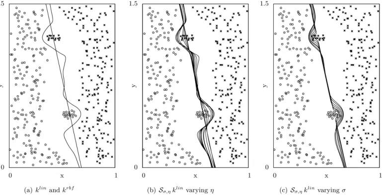
Figure 1: The separating hyperplanes for a two-feature hand-built artificial datasets defined by the application of the SVM (all with C = 3) with (a) linear kernel klin and RBF kernel
krbf (with γrbf = 150), (b) the S
σ,ηklin quasi-local kernel with fixed σ (σ = 1/150 =
1/γrbf) and variable η (η = 106, 50, 10, 1, 0.5, 0.1, 0.05, 0.03, 0.01, 0.005, 0.001, 0.000001), and (c) the Sσ,ηklin quasi-local kernel with fixed η (η = 0.05) and variable σ (σ =
1/5000, 1/2000, 1/1000, 1/500, 1/300, 1/150, 1/100).
The operators on kernels defined in the previous section aim to modify the behaviour of an input kernel k in order to produce a kernel more sensitive to local information in the feature space, maintaining however the original behaviour for regions in which the locality
is not important. In addition the η and σ parameters control the balance between the input kernel k and its local reformulation Eσk, in other words the effects of the local information.
These intuitions are highlighted in Figure 1 with an example that illustrates the ef-fects of the Sσ,η operator on the linear kernel klin using a two-feature hand-built artificial
dataset. We chose the linear kernel because its effects are easily recognizable in plots. The transformed kernel is:
(Sσ,ηklin)(x, x0) = klin(x, x0) + η · (Eσklin)(x, x0) = klin(x, x0) + η · krbf(x, x0) (11)
with γrbf = 1/σ. So the S
σ,η operator on the klin kernel gives a linear combination of klin
and krbf. Figure 1(a) shows the behaviour of only the global term klinand of only the local term Eσklin = krbf. Figure 1(b) illustrates what happens when the local and the global
terms are balanced with different values of η and a fixed σ. Figure 1(c) shows the behaviour of the separating hyperplane with a fixed balancing factor η but varying the σ parameter. The η parameter regulates the influence on the separating hyperplane of the local term of the quasi-local kernel. In fact, in Figure 1(b), we see that all the planes lie between the input kernel (klin, obtained with η → 0 from S
σ,ηklin) and the local reformulation
of the same kernel (obtained with η = 106 from S
σ,ηklin which behaves as krbf since the
high value of η partially hides the effect of the global term). Moreover, since σ is low, the modifications induced by different values of η are global, influencing all the regions of the separating hyperplane.
We can observe in Figure 1(c), on the other hand, that σ regulates the magnitude of the distortion from the linear hyperplane for the region containing points close to the plane itself. The σ parameter in the Eσklin term of Sσ,ηklin has a similar role to the
K parameter in the local SVM approach (i.e. it regulates the range of the locality), even though K defines an hard boundary between local and non local points instead of a negative exponential one. It is important to underline that in the central region of the dataset the separating hyperplane remains linear, highlighting that the kernel resulting from the Sσ,η
operator is able to modify the input kernel only where the information is local.
The example simply illustrates the intuition behind the proposed family of quasi-local kernels, and in particular how the input kernel behaviour is maintained for the regions in which the information is not local, so it is not important here to analyse the classification accuracy. However, kernels that are sensitive to important local information but retain properties of global input kernels, can also be obtained from very elaborated and well tuned kernels defined on high-dimensionality input spaces. Notice that in this toy example we are considering locality in input space since, using the linear kernel, the kernel trick is not applied. In the following two sections we investigate the accuracy performances of the quasi-local kernels in a number of real datasets using a data-dependent method of choosing η and σ parameters.
5
Experiment 1
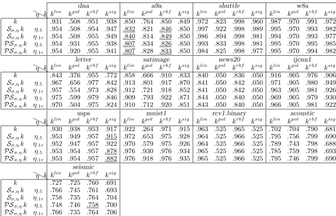
The first experiment consists in the evaluation of the accuracy of the quasi-local kernels with different but systematic choices of σ and η parameters on quite a large number of
datasets. The aim of the experiment is to understand which quasi-local kernels achieve better results with respect to the four reference input kernels. The implementation of the classifiers used in this work is based on the LibSVM library [7] version 2.84.
5.1 Experimental procedure
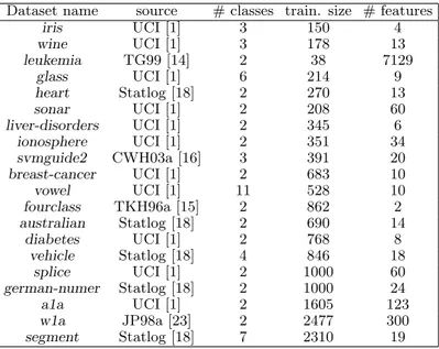
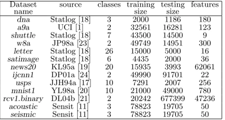
Table 1 lists the 20 datasets from different sources and scientific fields used in this exper-iment; some datasets are multiclass and the number of features ranges from 2 to 7129. All the datasets are collected and freely available online at the homepage of LibSVM [7]. They are small- or medium-size datasets permitting the Leave-One-Out (Loo) evaluation strategy for the classifiers which is a special case of the Cross Validation technique [31] consisting in testing every sample of the dataset with the classifier built on all the other points and averaging the correct classification cases with the dataset cardinality. The Loo is computationally expensive, but as shown in [32] it gives a good bound on the expectation of error for SVM. We denote with ALoo(ω, D) the Loo accuracy obtained by the ω classifier
on the D dataset.
The reference input kernels for the quasi-local operators considered are the linear kernel klin, the polynomial kernel kpol, the radial basis function kernel krbf and the sigmoidal
kernel ksig. The quasi-local kernels we tested are those resulting from the application of
the Eσ, Pσ, Sσ, Sσ,η, PSσ and PSσ,η operators on the reference input kernels. We also
evaluated the accuracy of the KNNSVM classifier with the same reference input kernels.
Dataset name source # classes train. size # features
iris UCI [1] 3 150 4 wine UCI [1] 3 178 13 leukemia TG99 [14] 2 38 7129 glass UCI [1] 6 214 9 heart Statlog [18] 2 270 13 sonar UCI [1] 2 208 60 liver-disorders UCI [1] 2 345 6 ionosphere UCI [1] 2 351 34 svmguide2 CWH03a [16] 3 391 20 breast-cancer UCI [1] 2 683 10 vowel UCI [1] 11 528 10 fourclass TKH96a [15] 2 862 2 australian Statlog [18] 2 690 14 diabetes UCI [1] 2 768 8 vehicle Statlog [18] 4 846 18 splice UCI [1] 2 1000 60 german-numer Statlog [18] 2 1000 24 a1a UCI [1] 2 1605 123 w1a JP98a [23] 2 2477 300 segment Statlog [18] 7 2310 19
Table 1: The 20 datasets for Experiment 1.
For the reference input kernels we set the parameters in the following way: for the polynomial kernel d = 3, γpol = p and rpol = 0, for the sigmoidal kernel rsig = 0. For
Eu-clidean distance between the samples of the datasets. For the quasi-local kernels obtained with the operators, the parameters to set are η and σ and we use the data-dependent estimation described in subsection 3.3; in particular we set η ∈ {η.1, η.5, η.9, η.1r, η.5r,
η.9r, ηF
.1, η.5F, η.9F} and σ = σ.1 without extensively use σ = σ.1F since preliminary tests
gave bad results for this setting. The C parameter of SVM is set to 1. Finally, the value of K in the KNNSVM classifier is automatically chosen on the training set between K = {1, 3, 5, 7, 9, 11, 15, 23, 39, 71, 135, 263, 519, 1031} (the first 5 odd natural numbers fol-lowed by the ones obtained with a base-2 exponential increment from 9) as described in section 2.2. We also evaluate KNNSVM without automatic K choice, i.e. with a-priori fixed values of K ∈ K.
In order to compare the quasi-local kernel results with the best potentially achievable results of the KNNSVM locality-based classifier, we compute the K that maximizes the Loo accuracy, denoted as K∗. Formally, K∗ is:
K∗ = argmin
K∈K
ALoo(KNNSVM, D).
So K∗NNSVM has the best Loo accuracy among the local SVM with fixed value of K, but
we remark that this a-posteriori choice of the best K for KNNSVM to obtain K∗NNSVM
is not a classification method because it uses information of test samples.
As stated above, the classification capability of an SVM with a kernel k on a specific dataset D, is evaluated considering the Loo accuracy, denoted by ALoo(SV M
k, D) or simply,
assuming that we use a kernel always through the SVM algorithm, ALoo(k, D). To assess the accuracy difference between two kernels in the same dataset, we can calculate the absolute difference between the Loo accuracies (both expressed in percentage):
∆ALoo(k1, k2, D) = (ALoo(k1, D) − ALoo(k2, D)) · 100
In order to make the ∆ALooindependent from the absolute values of the accuracies, we also
introduce the relative percentage difference of Loo accuracy: δALoo(k1, k2, D) = ∆A
Loo(k1, k2, D)
ALoo(k2, D)
Applying δALoo(k1, k2, D) (or ∆ALoo(k1, k2, D)) on a considerable number of datasets D with
k1 = O k the kernel obtained with the application of the operator O on the input kernel k and k2 = k, we can obtain a distribution of relative (or absolute) Loo accuracy differences
between O k and k. On this distribution we compute descriptive statistics; the mean, the standard deviation (sd) and the skewness (skew). By means of box-plot diagrams, we show the median, the first quartile, the third quartile, the whiskers (i.e. the maximum value within the third quartile plus 1.5 times the interquartile range and the minimum value within the first quartile minus 1.5 times the interquartile range), and the extreme or outlier values (i.e. values that are over the third quartile plus 1.5 times the interquartile range or under the first quartile minus 1.5 times the interquartile range). Moreover, we define νδ>t
to be the percentage of datasets in which the relative percentage difference δALoo between
O k and k is greater than a fixed threshold t: νδ>t= |{Di | δA
Loo(O k, k, Di) > t}|
nD · 100 i = 1, . . . , nD
where nD is the total number of datasets considered. Similarly the percentage of datasets in which the relative percentage difference between O k and k is negative and lower than a threshold -t is:
νδ<-t= |{Di | δA
Loo(O k, k, Di) < -t}|
nD · 100 i = 1, . . . , nD.
Representing the accuracy values of O k and k on a scatter plot, νδ>t and νδ<-t with t = 0
can be seen as the number of points lying over and under the bisector line (y = x), i.e. the number of datasets in which the quasi-local kernels perform better and worse with respect to the input kernels. With non-zero values for t, the graphical meaning of νδ>tand νδ<-t is
the number of points lying over y = x · (1 + t/100) and under y = x · (1 − t/100). 5.2 Results
segment sonar vehicle splice
H
Hη k klin kpol krbf ksig klin kpol krbf ksig klin kpol krbf ksig klin kpol krbf ksig
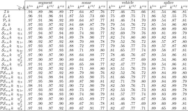
I k .94 .89 .96 .89 .77 .64 .87 .76 .77 .46 .75 .66 .81 .54 .86 .81 Eσk .96 .91 .96 .91 .87 .53 .73 .60 .75 .49 .75 .71 .86 .52 .55 .75 Pσk .97 .91 .96 .92 .89 .64 .87 .77 .81 .46 .74 .70 .89 .54 .87 .81 Sσk .97 .93 .97 .92 .84 .68 .87 .79 .79 .54 .76 .72 .85 .54 .86 .80 Sσ,ηk η.1 .97 .93 .97 .92 .88 .71 .91 .79 .78 .54 .77 .73 .89 .80 .89 .80 Sσ,ηk η.5 .97 .94 .97 .94 .89 .74 .90 .77 .82 .69 .79 .76 .89 .81 .89 .79 Sσ,ηk η.9 .97 .96 .97 .94 .89 .78 .90 .77 .82 .74 .80 .80 .89 .82 .88 .81 Sσ,ηk η.1r .96 .92 .97 .92 .88 .70 .88 .78 .79 .52 .76 .72 .88 .57 .87 .80 Sσ,ηk η.5r .97 .93 .97 .93 .88 .72 .89 .77 .79 .56 .77 .73 .89 .57 .87 .80 Sσ,ηk η.9r .97 .94 .97 .93 .88 .71 .89 .80 .81 .65 .77 .74 .89 .58 .87 .81 Sσ,ηk η.1F .97 .90 .97 .90 .88 .64 .88 .77 .78 .46 .76 .67 .89 .54 .86 .81 Sσ,ηk η.5F .97 .90 .97 .90 .89 .64 .88 .77 .82 .47 .77 .69 .89 .54 .86 .80 Sσ,ηk η.9F .97 .91 .97 .92 .89 .65 .88 .77 .82 .47 .77 .70 .89 .54 .86 .81 PSσk .97 .92 .97 .92 .89 .71 .88 .80 .83 .51 .76 .73 .88 .71 .88 .81 PSσ,ηk η.1 .97 .92 .97 .92 .89 .79 .90 .76 .82 .52 .76 .72 .89 .84 .89 .80 PSσ,ηk η.5 .97 .94 .98 .94 .89 .83 .90 .75 .81 .66 .79 .77 .89 .84 .89 .80 PSσ,ηk η.9 .97 .95 .98 .95 .89 .87 .90 .81 .82 .71 .79 .80 .89 .84 .89 .79 PSσ,ηk η.1r .98 .91 .97 .92 .90 .72 .90 .79 .82 .50 .76 .71 .89 .82 .89 .79 PSσ,ηk η.5r .97 .93 .97 .93 .89 .73 .90 .77 .82 .53 .76 .73 .89 .83 .89 .78 PSσ,ηk η.9r .97 .94 .98 .93 .90 .74 .90 .79 .81 .57 .77 .74 .89 .83 .89 .79 PSσ,ηk η.1F .97 .90 .97 .90 .89 .65 .89 .77 .82 .46 .76 .67 .89 .56 .89 .81 PSσ,ηk η.5F .97 .90 .97 .90 .89 .67 .91 .78 .81 .46 .77 .69 .89 .60 .89 .81 PSσ,ηk η.9F .97 .91 .97 .92 .89 .67 .91 .77 .82 .47 .77 .71 .89 .65 .89 .81
Table 2: Experiment 1. Loo accuracy of input kernels ALoo(I k, D) and of quasi-local
kernels ALoo(O k, D) on segment, sonar, vehicle and splice datasets.
Table 2 presents the Loo accuracy values for the segment, sonar, vehicle and splice datasets. These four datasets were arbitrarily selected for their representativeness. For
space reasons, the accuracy results of the remaining datasets are available in the Additional Material. Formally the table shows the ALoo(O k, D) values using O ∈ {I, E
σ, Pσ, Sσ, Sσ,η, PSσ, PSσ,η}
with σ = σ.1 and η ∈ {η.1, η.5, η.9, η.1r, η.5r, η.9r, η.1F, η.5F, ηF.9}, k ∈ {klin, kpol, krbf, ksig},
D ∈ {segment, sonar, vehicle, splice}.
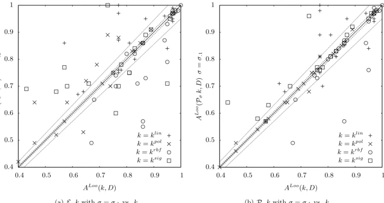
0.4 0.5 0.6 0.7 0.8 0.9 1 0.4 0.5 0.6 0.7 0.8 0.9 1 A Loo (Eσ k ,D ) σ = σ.1 ALoo(k, D) k = klin k = kpol k = krbf k = ksig (a) Eσk with σ = σ.1vs. k 0.4 0.5 0.6 0.7 0.8 0.9 1 0.4 0.5 0.6 0.7 0.8 0.9 1 A Loo (P σ k ,D ) σ = σ.1 ALoo(k, D) k = klin k = kpol k = krbf k = ksig (b) Pσk with σ = σ.1vs. k
Figure 2: Experiment 1. Scatter plots for the Loo accuracy comparison between Eσk and
Pσk quasi-local kernels and the corresponding input kernels k with k ∈ {klin, kpol, krbf, ksig}
for all the 20 datasets.
Considering all the 20 datasets of experiment 1, the scatter plots in Figure 2 and Figure 3 summarize the results for the Eσk, Pσk, Sσ,ηk and PSσ,ηk quasi-local kernels with η = η.5
and σ = σ.1 comparing their Loo accuracies with those of the corresponding input kernels.
Points over the bisector line mean accuracy improvements of quasi-local kernels with respect to the input kernels, the opposite for points under the bisector line. The dotted lines denote accuracy deviations of 1% and 5% from the bisector line, i.e. the limits defined by νδ>tand νδ<-t with t = 1 and t = 5.
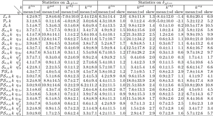
Table 3 and the box-plots of Figure 4 report the statistics on the differences between the Loo accuracies of the quasi-local kernels and the corresponding input kernels. Table 3 presents the mean and the standard deviation (sd) of the distribution of the absolute differences ∆ALoo(O k, k, D), and the mean, the standard deviation (sd) and the skewness
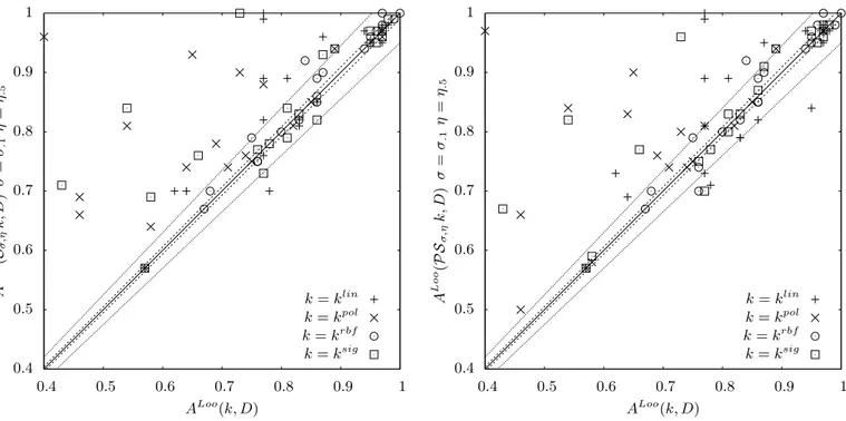
0.4 0.5 0.6 0.7 0.8 0.9 1 0.4 0.5 0.6 0.7 0.8 0.9 1 A Loo (Sσ ,η k ,D ) σ = σ.1 η = η.5 ALoo(k, D) k = klin k = kpol k = krbf k = ksig
(a) Sσ,ηk with σ = σ.1 and η = η.5 vs. k
0.4 0.5 0.6 0.7 0.8 0.9 1 0.4 0.5 0.6 0.7 0.8 0.9 1 A Loo (P Sσ ,η k ,D ) σ = σ.1 η = η.5 ALoo(k, D) k = klin k = kpol k = krbf k = ksig (b) PSσ,ηk with σ = σ.1and η = η.5vs. k
Figure 3: Experiment 1. Scatter plots for the Loo accuracy comparison between Sσ,ηk and PSσ,ηk quasi-local kernels and the corresponding input kernels k with k ∈
{klin, kpol, krbf, ksig} for all the 20 datasets.
of Experiment 1. Figure 4 shows graphically, by means of box-plots, the median, the first quartile, the third quartile, the whiskers and the extreme values of the relative Loo differences.
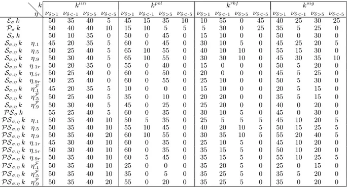
Table 4 reports the percentages of datasets in which the quasi-local kernels achieve substantially better results, in terms of Loo accuracy relative differences, with respect to the corresponding input kernel, formally νδ>t, and in which they perform substantially
worse, formally νδ<-t. For example, for t = 5 and for the kernel resulting from Sσ,η with
σ = σ.1 and η = η.5, we have that the accuracy is never worse than 5% of the input
kernels (except for one dataset in the linear kernel case) while the percentages of datasets in which we have a gain in accuracy of at least 5% are 40% for the linear kernel, 55% for the polynomial kernel, 10% for the RBF kernel and 30% for the sigmoidal kernel.
The input-space estimated values of the dataset-dependent parameter used in this ex-periment (σ.1 = η.1, η.5, η.9, η.1r, η.5r, η.9r) are reported in the Additional Material for every
dataset of Experiment 1; here we notice that the ratios between η.5 and η.1r are about of
one order of magnitude. In particular the median of the ratios is 6.5, the first quartile is 4.5, the third quartile is 9.4; in only one case (svmguide2 dataset) is η.5lower than η.1rand
Statistics on ∆ALoo Statistics on δALoo
klin kpol krbf ksig klin kpol krbf ksig
@
@k
η mean±sd mean±sd mean±sd mean±sd mean±sd skew mean±sd skew mean±sd skew mean±sd skew Eσk 4.2±9.7 2.8±6.6 -7.0±10.0 2.4±12.6 6.3±14.4 2.0 4.9±11.8 1.3 -8.4±12.0 -1.4 6.0±20.4 6.0 Pσk 3.1±8.5 0.1±1.6 -4.0±8.2 3.0±6.6 4.3±10.8 1.0 0.1±2.4 -0.9 -5.0±10.0 -2.1 5.2±12.2 5.2 Sσk 5.1±8.7 5.3±6.3 0.1±0.8 6.0±9.4 7.4±13.5 2.3 9.8±12.9 1.4 0.1±1.0 0.2 10.5±17.8 10.5 Sσ,ηk η.1 3.7±7.1 5.7±7.5 0.9±2.1 3.4±7.3 4.9±9.2 1.5 10.6±15.6 2.0 1.0±2.4 2.3 5.8±12.6 5.8 Sσ,ηk η.5 4.1±7.8 10.8±14.1 1.1±2.2 5.6±10.4 5.4±10.1 1.2 21.3±33.2 2.5 1.2±2.6 1.8 9.9±19.5 9.9 Sσ,ηk η.9 4.2±8.1 12.6±14.7 0.6±2.7 5.6±11.6 5.7±10.7 1.1 24.1±34.2 2.2 0.6±3.3 1.1 10.0±21.0 10.0 Sσ,ηk η.1r 3.9±6.7 3.9±4.5 0.3±0.6 3.8±7.3 5.2±8.7 1.7 6.9±8.5 1.1 0.3±0.7 1.1 6.4±13.2 6.4 Sσ,ηk η.5r 4.3±7.1 6.5±7.9 0.4±0.9 4.9±8.9 5.9±9.4 1.4 12.5±17.8 2.2 0.4±1.1 1.1 8.6±16.7 8.6 Sσ,ηk η.9r 4.8±7.6 8.5±11.8 0.3±1.1 5.5±9.6 6.7±10.5 1.2 17.0±28.2 2.8 0.3±1.3 0.6 9.7±18.2 9.7 Sσ,ηk ηF.1 3.7±7.1 0.3±0.4 0.2±0.9 0.9±2.4 4.9±9.2 1.5 0.4±0.6 2.0 0.2±1.0 0.3 1.7±4.1 1.7 Sσ,ηk ηF.5 4.1±7.8 0.9±1.3 0.1±1.2 2.7±6.6 5.4±10.1 1.2 1.4±2.3 1.9 0.1±1.5 0.3 4.5±10.6 4.5 Sσ,ηk ηF.9 4.2±8.1 2.2±3.5 0.1±1.2 3.8±8.0 5.7±10.7 1.1 3.4±5.4 1.6 0.1±1.5 0.2 6.6±14.7 6.6 PSσk 4.3±7.7 4.0±5.4 0.7±1.9 4.5±7.8 5.8±10.2 1.2 7.1±9.5 1.7 0.8±2.3 2.9 7.8±14.8 7.8 PSσ,ηk η.1 3.0±7.8 5.1±8.6 0.8±2.3 2.4±5.3 4.2±9.9 0.8 9.6±15.8 1.9 0.9±2.7 1.1 4.1±9.7 4.1 PSσ,ηk η.5 3.2±8.9 8.8±14.5 0.7±2.7 4.6±9.4 4.4±11.5 1.0 18.0±33.9 2.8 0.8±3.3 0.1 8.0±17.4 8.0 PSσ,ηk η.9 3.0±9.0 10.9±14.6 0.2±2.9 6.2±11.2 4.2±11.5 1.0 21.5±33.8 2.4 0.1±3.6 0.5 10.8±20.8 10.8 PSσ,ηk η.1r 3.1±8.0 4.3±7.4 0.7±2.0 2.6±4.8 4.4±10.2 0.7 7.6±13.3 2.6 0.8±2.4 2.6 4.5±9.1 4.5 PSσ,ηk η.5r 3.5±8.6 5.3±8.1 0.7±2.1 3.9±7.6 4.9±11.1 0.9 9.8±15.3 1.9 0.8±2.5 2.2 6.7±14.3 6.7 PSσ,ηk η.9r 3.4±8.7 6.1±8.5 0.8±2.1 4.8±8.9 4.8±11.3 1.0 11.5±16.8 1.7 0.9±2.6 2.0 8.4±16.6 8.4 PSσ,ηk ηF.1 3.0±7.8 0.5±0.8 0.6±2.1 0.6±1.3 4.2±9.9 0.8 0.7±1.3 2.1 0.7±2.5 2.5 1.0±2.3 1.0 PSσ,ηk ηF.5 3.2±8.9 0.9±1.5 0.7±2.3 2.1±4.9 4.4±11.5 1.0 1.5±2.6 2.7 0.7±2.8 1.6 3.4±7.7 3.4 PSσ,ηk ηF.9 3.0±9.0 1.7±2.5 0.6±2.4 3.3±7.1 4.2±11.5 1.0 2.9±4.7 2.9 0.7±2.8 1.6 5.7±12.6 5.7
Table 3: Experiment 1. Mean and standard deviation of the absolute differences, and mean, standard deviation and skewness of the relative differences between Loo accuracies of quasi-local kernels and of corresponding input kernels, for all the 20 datasets.
in only one case (leukemia dataset) is the ratio greater then 100.
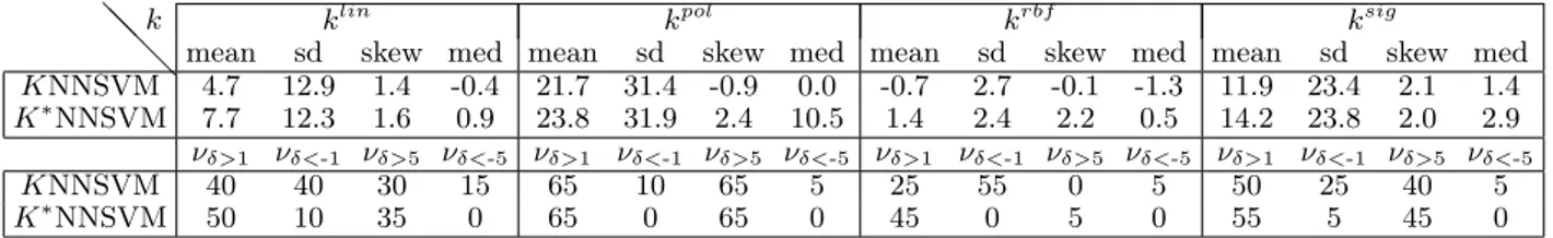
Table 5 shows the Loo accuracy of the KNNSVM classifier and of the KNNSVM clas-sifier with fixed a-priori K values for the segment, sonar, vehicle and splice datasets (the results for all the datasets are available in the Additional Material). Obviously for values of K in KNNSVM greater than the dataset cardinality the accuracy results are missing. Similarly to the classifier accuracy statistics reported in Table 3 and Table 4, the KNNSVM classifier and the K∗NNSVM values are also summarized in Table 6 using the relative Loo
accuracy values.
Finally, the scatter plot in Figure 5 compares the performance of the Sσ,ηk with η.5and
σ.1 with the KNNSVM classifier and with K∗NNSVM for every dataset.
5.3 Discussion
Observing the box-plots diagrams of Figure 4 regarding the relative variation in the Loo accuracy produced by the quasi-local kernels in the SVM classification, we can see that most of the quasi-local kernels are able to significantly improve the classification accuracy of the reference input kernels. The same conclusion can be deduced from Table 4 in which, apart from Eσk and Pσk with k = krbf, the quasi local kernels exhibit always a higher (or
klin kpol krbf ksig @ @k η νδ>1 νδ<-1 νδ>5 νδ<-5 νδ>1 νδ<-1 νδ>5 νδ<-5 νδ>1 νδ<-1 νδ>5 νδ<-5 νδ>1 νδ<-1 νδ>5 νδ<-5 Eσk 50 35 40 5 45 15 35 10 10 55 0 45 40 25 30 25 Pσk 50 40 40 10 15 10 5 5 5 30 0 25 35 5 25 0 Sσk 50 10 35 0 50 0 45 0 15 10 0 0 50 0 30 0 Sσ,ηk η.1 45 20 35 5 60 0 45 0 30 10 5 0 45 25 20 5 Sσ,ηk η.5 50 25 40 5 65 10 55 0 40 10 10 0 55 15 30 0 Sσ,ηk η.9 50 30 40 5 65 10 55 0 30 30 10 0 45 30 35 10 Sσ,ηk η.1r 50 20 35 0 55 0 40 0 15 0 0 0 50 5 20 0 Sσ,ηk η.5r 50 25 40 0 60 0 50 0 20 0 0 0 45 5 25 0 Sσ,ηk η.9r 50 25 40 0 60 0 55 0 25 10 0 0 50 5 30 0 Sσ,ηk ηF.1 45 20 35 5 10 0 0 0 15 10 0 0 20 5 15 0 Sσ,ηk ηF.5 50 25 40 5 35 0 10 0 20 20 0 0 35 5 15 0 Sσ,ηk ηF.9 50 30 40 5 45 0 25 0 25 20 0 0 40 0 20 0 PSσk 55 25 40 5 60 0 35 0 30 10 5 0 45 0 30 0 PSσ,ηk η.1 50 35 40 10 50 5 35 0 25 5 5 5 45 10 20 5 PSσ,ηk η.5 50 35 40 10 55 10 45 0 40 20 10 5 50 15 25 5 PSσ,ηk η.9 50 35 40 20 60 10 55 0 30 35 10 5 55 20 40 5 PSσ,ηk η.1r 45 30 40 10 60 0 35 0 25 10 5 0 45 10 20 0 PSσ,ηk η.5r 50 30 40 10 60 0 35 0 35 15 5 0 50 10 20 0 PSσ,ηk η.9r 50 35 40 10 60 5 45 0 35 15 5 0 55 10 25 5 PSσ,ηk ηF.1 50 35 40 10 25 0 0 0 35 20 5 0 25 0 15 0 PSσ,ηk ηF.5 50 35 40 10 35 0 5 0 35 25 5 0 35 5 20 0 PSσ,ηk ηF.9 50 35 40 20 55 0 20 0 35 25 5 0 35 0 20 0
Table 4: Experiment 1. Table of the percentages of datasets νδ>t (and νδ<−t) in which the quasi-local kernels achieve sensibly better (and worse) Loo accuracy values with respect to to the corresponding input kernels. Thresholds of 1% and 5% are considered.
showing accuracy losses. More precisely, analysing also the mean relative Loo variations in Table 3, the quasi-local kernels that are shown to be more accurate are Sσ, Sσ,η with
η ∈ {η.1, η.5, η.9, η.1r, η.5r, η.9r}, PSσ and PSσ,η with η ∈ {η.1, η.5, η.9, η.1r, η.5r, η.9r}
all with σ = σ.1. All their Loo variations are in fact positive, and observing that also the skewness is always positive, the standard deviation is rather high because of positive outliers. On the other hand, the kernels resulting from Eσ shows important limitations, as
reported in Table 4; for example only 45% of the datasets do not give accuracy values lower than 1% of the accuracy of the RBF kernel, meaning that in 55% of cases the results are lower than 1%. The only case in which Eσk seem to perform quite well is with the linear
kernel as input kernel, but this is not surprising since Eσklin= krbf. Kernels obtained from
Pσ are even worse than the one produced by Eσ. The low Loo accuracy results of Eσ and
Pσ are also highlighted by the scatter plots of Figure 2, in which it is clear that there is
not a predominance of points over the bisector line.
For Sσ,η the best results in terms of Loo accuracy improvements are achieved for η.1,
η.5 and η.9 and in general Sσ,ηk gives Loo accuracy values higher than PSσ,ηk as we can
see especially in Table 3. In contrast, the quasi-local kernels that seem to guarantee less risk of achieving worse results are those obtained from Sσ,η with η.1r, η.5r and η.9r (see
the percentages of relative Loo accuracy losses in Table 4). So we can reasonably conclude that the quasi-local kernel that seems more promising are produced by the operators Sσ,η
segment sonar vehicle splice H
H k klin kpol krbf ksig klin kpol krbf ksig klin kpol krbf ksig klin kpol krbf ksig
KNNSVM .97 .97 .97 .97 .88 .80 .85 .84 .70 .69 .70 .71 .77 .63 .86 .85 1-NNSVM .97 .97 .97 .97 .88 .80 .88 .87 .70 .69 .70 .70 .70 .61 .70 .71 3-NNSVM .97 .96 .96 .97 .86 .79 .84 .85 .71 .71 .70 .71 .70 .63 .70 .70 5-NNSVM .96 .96 .96 .96 .88 .78 .82 .81 .72 .71 .70 .72 .72 .57 .70 .70 7-NNSVM .95 .95 .96 .95 .89 .77 .80 .80 .72 .70 .71 .72 .72 .48 .71 .71 9-NNSVM .95 .95 .96 .95 .89 .72 .76 .77 .72 .71 .70 .71 .75 .48 .71 .71 11-NNSVM .95 .95 .95 .95 .91 .68 .81 .72 .72 .69 .72 .70 .75 .48 .71 .70 15-NNSVM .95 .95 .96 .95 .88 .67 .83 .73 .72 .69 .72 .69 .77 .64 .73 .72 23-NNSVM .95 .94 .97 .94 .87 .67 .86 .72 .74 .66 .73 .68 .78 .57 .75 .73 39-NNSVM .95 .92 .97 .93 .89 .67 .88 .75 .74 .64 .74 .67 .79 .48 .77 .78 71-NNSVM .95 .89 .97 .90 .88 .64 .89 .75 .76 .59 .75 .63 .80 .49 .83 .83 135-NNSVM .95 .86 .97 .88 .80 .59 .88 .79 .78 .55 .75 .61 .78 .48 .85 .85 263-NNSVM .95 .86 .97 .89 - - - - .80 .49 .75 .67 .79 .48 .86 .82 519-NNSVM .94 .88 .96 .89 - - - - .79 .43 .75 .69 .77 .48 - .86 .80 1031-NNSVM .94 .90 .96 .90 - - -
-Table 5: Experiment 1. Loo accuracy result of the KNNSVM classifier and of KNNSVM classifier with fixed a-priori values of K. KNNSVM results for K greater than the dataset cardinality are missing because the classifier is not applicable. The K∗NNSVM values are
highlighted in bold.
klin kpol krbf ksig
@ @
@k
mean sd skew med mean sd skew med mean sd skew med mean sd skew med
KNNSVM 4.7 12.9 1.4 -0.4 21.7 31.4 -0.9 0.0 -0.7 2.7 -0.1 -1.3 11.9 23.4 2.1 1.4
K∗NNSVM 7.7 12.3 1.6 0.9 23.8 31.9 2.4 10.5 1.4 2.4 2.2 0.5 14.2 23.8 2.0 2.9
νδ>1 νδ<-1 νδ>5 νδ<-5 νδ>1 νδ<-1 νδ>5 νδ<-5 νδ>1 νδ<-1 νδ>5 νδ<-5 νδ>1 νδ<-1 νδ>5 νδ<-5
KNNSVM 40 40 30 15 65 10 65 5 25 55 0 5 50 25 40 5
K∗NNSVM 50 10 35 0 65 0 65 0 45 0 5 0 55 5 45 0
Table 6: Experiment 1. Mean, standard deviation, skewness and median of relative Loo accuracy differences between SVM using the input kernels and the KNNSVM classifier and with K∗NNSVM on all the 20 datasets.
with η.5 and σ.1 and Sσ,η with η.1r and σ.1; in particular the first is the one that appear to
potentially achieve better results, while the second is the one with less possibility to achieve worse results. In addition, the performances of the PSσ,η derived class of kernels are very close to the Sσ,η ones, although they are a bit lower. The fact that η.5 is statistically almost
10 times greater than η.1rconfirms the observation that Sσ,ηk and PSσ,ηk with η = η.1rare
more conservative with respect to the k input kernel behaviour than the same quasi-local kernels with η = η.5 and make reasonable the use of both parameter settings.
The resulting statistics (see for example the box-plots in Figure 4) show that all the input kernels benefit from the quasi-local transformation by the Sσ, Sσ,η, PSσ and PSσ,η operators. However, the quasi-local kernels with lower accuracy improvements are those applied on the RBF input kernel (they rarely improve the krbf accuracy by more than 5%
as reported in Table 4). This is reasonable since the RBF kernel is already a local kernel and thus should not take advantage of the operator transformation, so even the small improvements observed are very positive. The explanation for the accuracy improvements