UNIVERSITY
OF TRENTO
DEPARTMENT OF INFORMATION AND COMMUNICATION TECHNOLOGY
38050 Povo – Trento (Italy), Via Sommarive 14
http://www.dit.unitn.it
An Efficient Scheduling Algorithm for Time-Driven Switching
Networks
Thu-Huong Truong, Mario Baldi, Yoram Ofek
January 2007
1
Abstract— In Time-driven Switching (TDS) networks with non-immediate forwarding (NIF) provides scheduling flexibility and consequently, reduces the blocking probability (blocking is defined to take place when transmission capacity is available, but without a feasible schedule). However, it has been shown that with NIF scheduling complexity may grow exponentially. Efficiently finding a schedule from an exponential set of potential schedules is the focus of this paper. The work first presents the mathematical formulation of the NIF scheduling problem, under a wide variety of networking requirements, then introduces an efficient (i.e., having at most polynomial complexity) search algorithm that guarantees to find at least one schedule whenever such a schedule exists. The novel algorithm uses ‘trellis’ representations and the well-known survivor-based searching principle.
Index Terms— scheduling, search algorithms, time-driven
switching, pipeline forwarding, optical networks
I. INTRODUCTION
cheduling for flexible bandwidth provisioning in heterogeneous networks while satisfying various service requirements is critical in next generation networking. The main context of this work is time-driven Switching (TDS), see [1]-[6], which is a scalable switching design based on UTC (Coordinated universal time) with pipeline forwarding. Under the pipeline forwarding principle packets are forwarded in time frames (TFs) in a “lock-step” manner across the route. TDS enables deterministic performance guarantees, flexible bandwidth provisioning, and low cost switching scalability.
Pipeline forwarding at a TDS switch can be performed in two manners (1) immediate forwarding (IF) and (2) non-immediate forwarding (NIF). IF is simple but provides a smaller number of different pipeline forwarding schedules, and consequently, may result in high blocking probability (blocking is defined as an event in which transmission capacity is available without a feasible schedule). On the other hand, NIF provides higher scheduling flexibility as the number of possible schedules growing exponentially with the
number of hops, and consequently, significantly reducing the blocking probability. The complexity of TDS scheduling problem depends on various factors, such as, the forwarding schemes (IF, NIF), the network dimension (the number of switches, the number of wavelengths per optical fiber), the predefined technology parameters (link bandwidth, the duration of time frames and time cycles).
The schedule search algorithm presented in [2] is suitable only for the simple IF case of single channel per link, not dealing with the complexity introduced by WDM and NIF, which is the focus of this paper. The work [7] addresses the RWTA (Route, Wavelength, Time slot Assignment) problem in time-shared wavelength-routed WDM networks. Although this has similarities with the scheduling task in TDS networks, [7] only deals with a scenario that is comparable to the IF case. Scheduling a scenario, featuring IF and no wavelength conversion has lower complexity (time slot and wavelength assignment) but less scheduling/provision flexibility.
Within the scope of this paper, we will present an efficient algorithm for the NIF problem of time frame scheduling over a predefined route with extensions to multiple-wavelength. The paper is organized as follows: Section II formulates our problem and shows the way that led to our proposed solution. In Section III, we first present an algorithm for the fundamental case of single-TF request in a single-channel, homogeneous network (all links have the same capacity). A special graph, i.e. a trellis, is constructed and used by the search algorithm that is motivated by the Viterbi algorithm [10] and compared with the well known Dijkstra algorithm [11][12]. Section IV extends the solution to the more complicated case of WDM homogeneous networks. Finally, we discuss further extensions of this work in Section V.
II. SCHEDULING PROBLEM FORMULATION AND SCOPE This work focuses on a time-driven switching (TDS) network with an arbitrary topology, where each optical link transports one or more optical channels (lambdas) with defined transmission bit rates. The TDS network operation principles were described in depth in [2]. The following is a brief summary that is needed for understanding of our scheduling search design and analysis.
An Efficient Scheduling Algorithm for
Time-Driven Switching Networks
Thu-Huong Truong♦ , Mario Baldi∗, Yoram Ofek♦
♦Department of Information and Communication Technology
University of Trento, Italy Email: (huong.truong, ofek)@dit.unitn.it
∗Control and Computer Engineering Department
Politechnico di Torino, Italy Email: [email protected]
A. TDS Network principle
Time Structure: TDS network uses common time reference
(CTR) that is commonly realized by using UTC (coordinated universal time). UTC is available everywhere through GPS and Galileo in the near future with accuracy that is well below 1µs. As Figure 1 depicts, the standard UTC second is divided into equal duration time frames (TFs), which are grouped into time cycles (TCs), such that, multiple contiguous TCs are equal to one UTC second. TFs are used to align and forward multi-protocol packets between switches. The TF capacity is calculated according to its duration and the link bandwidth. In this work there are K TFs per TC and all links are having the same TC duration.
Figure 1- Time structure and pipeline forwarding
Pipeline Forwarding: The basic principle of TDS network
operation is pipeline forwarding (PF), in which packets are forwarded in TFs with a predefined forwarding schedule that is responsive to UTC and without header processing. Consequently, TFs can be viewed as virtual containers of packets. The necessary condition for pipeline forwarding is having delay among inputs of TDS switches as an integer number of TFs. In order to realize this all incoming TFs should be aligned with UTC. However, without loss of generality, in this work we presume the availability of this alignment operation and ignore the propagation delay.
Pipeline forwarding delay is the delay of one hop measured in TFs between the inputs of two neighboring switches on a route from source to destination. In fact, the forwarding delay comprises of the propagation delay and the necessary UTC alignment delay (which we assume to be zero in the following analysis) and the Z-forwarding delay, which is the scheduling delay that is due to holding the incoming TF (with its packets) for the duration of Z TFs before forwarding to the next TDS switch on the route.
The Z-forwarding has two basic cases, as shown in Figure 1: 1. Z=0 - IF: incoming TFs are forwarded with zero delay to
the next switch on the route of h hops.
2. K>Z>0 - NIF: incoming TFs can be forwarded to the next TDS switch on the route of h hops with delay that is up to
Z TFs, i.e 0 TF (like in IF) or 1 TF or … or Z TFs.
The case of Z=K-1 is called full forwarding (FF) since the incoming TF can be forwarded after 0 TF (like in IF) or 1 TF or … or K-1 TFs. The case of IF provides no freedom in selecting TF sequence at every switch along the route. Once a TF is selected at the first switch on the route all subsequent TFs are determined. Meanwhile, the case of FF is trivial for scheduling since it always brings schedules as long as resource is still available. Therefore, this work focuses on NIF, since it brings more scheduling flexibility and scalability, reducing blocking probability and increasing network utilization.
B. TDS scheduling problem
Definitions:
Available TF - a TF at an output of a switch that can
participate in carrying packets of a requested flow.
Choice - a choice is an available output TF selected for a
given flow for which a set-up request arrived at a switch. A choice is limited by the constraint: if at switch j, TF i (0 ≤ i ≤
K-1) is assigned, then at switch j+1, a TF in the range of [i,
(i+Z)mod K] (in the same or the next TC) can be used.
Schedule - a schedule is a sequence of choices over a
predefined route of multiple switches.
Blocking of a schedule - a schedule is blocked at switch j
when no choice is possible on that switch to advance the schedule to the next switch.
1. Network model: In TDS, routes are determined for any
flow using exiting routing protocols. TDS then focuses on the manner of (pipeline) forwarding the packets on that route. Hence, we will only study here the TDS problem as specified in Figure 1: (1) on one predefined route (without route selection) with a predefined number of TDS switches as in Figure 2, (2) without propagation delay and alignment delay.
Figure 2 – Network model with Z=2-forwarding In fact, the buffered delay at each switch can be elastic in Z-range (Z at maximum); however once a schedule is fixed, each switch will forward packets strictly at the selected TF according to the selected schedule. The route is to carry traffic of the flow from Source to Destination via h TDS switches
2. Scheduling problem formulation: For NIF, sufficient
bandwidth (available TFs) on every switch does not guarantee a non-blocking schedule to setup a connection or a flow, due to the mapping range restricted within Z TFs forwarding. TFs on a switch in general are assumed to be randomly available since the flows are stochastically selected; thus all its available TFs may happen to be out of the Z-range for the considered request from the previous switch. Moreover, scheduling for NIF is a complicated task due to the larger size of the possible solution space, i.e., the large number of possible schedules as described below.
Observation 1: For Z-forwarding (0<Z<K-1), with a
single-channel, the total number of possible schedules for a h-hop route is: K⋅
(
Z+1)
h−1Proof: There are K choices for the 0th hop to forward a TF to
the 1st hop of the defined route. At the consecutive (h-1) hops,
3 all hop except the 0th one, there are (Z+1) choices to schedule
a TF. Since scheduling at all hops is independent (within the choice constraints), the total schedules are given by combination of all the possible single hop schedules:
( )
(
)
1 1 1 0 ( 1) ...( 1) 1 − − = ⋅ + + + ⋅ h h K Z Z Z K th st thThere is the difference in complexity between NIF and IF which has only K possible schedules with K TFs per TC. For one flow, finding a proper schedule from a space of
(
+1)
−1 ⋅ Z hK possibilities is a potentially complex problem due to the exponential boom of computations. A simple search for each request may take a long duration. Since we need to setup the flow (i.e., “virtual circuit”) before starting the data transfer, the search time could limit reducing the TF duration, and reducing the flexibility of the TDS network (as the optical channel capacity increases, then K and Z may increase as well). Moreover, with h in the exponent, the number of schedules grows exponentially with the size of the network.
Observation 2: For Z-forwarding (0<Z<K-1), with C optical
channels, the total number of possible schedules along a h-hop route is: K⋅
(
Z +1)
h−1⋅ChProof: the result is easily derived from the Observation 1
(
)
[
] [
]
(
)
h h h K Z C C Z C Z C K⋅ 0th⋅( +1)⋅ 1st...( +1)⋅ −1th = ⋅ +1 −1⋅Observation 1 and 2 show the exponential growth in the number of possible schedules. Thus, our objective is to design a scheduling algorithm that is efficient (low complexity) and robust, such that, it guarantees to find a schedule even if only one such schedule exists. Moreover, it may be important to minimize end-to-end delay by minimizing Z. This, in turn, will lead to minimizing the required buffer size.
In general, a flow may be allocated a bandwidth of: (i) one TF, (ii) multiple TFs or (iii) a fraction of TF, thus the scheduling algorithm should be able to allocate such the schedules, accordingly. However, in this work we focus on the one-TF scheduling case. We propose an algorithm based on using Viterbi algorithm [10], exploiting trellis diagrams. Thanks to their deterministic attributes, TDS resources on the route can be mapped to a suitable trellis structure to enable the search in dynamic stages. Also, from the analysis of different scenarios, the trellis will be adapted to each scenario with reasonable modifications. The scheduling algorithm is called eSS algorithm (efficient-with-Survivor-based-Search) and finds the same best schedule returned by exhaustive search, while not suffering from the exponential growth in schedule options due to the deployment of a survivor-based mechanism. Within the scope of this paper, we address to the scenario of scheduling for a Single TF request in Single/Multiple-Wavelength Homogeneous TDS networks.
III. ESS -EFFICIENT-WITH-
S
URVIVOR-BASED-S
EARCHA. Underlying principles
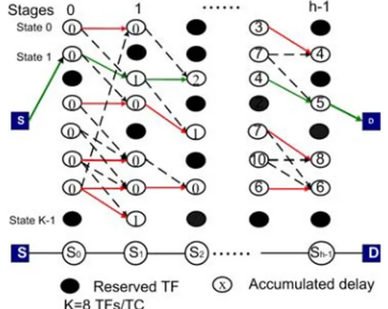
A trellis diagram is used to describe all possible schedules setup in the TDS network for a given requested flow. The eSS algorithm then searches for the best schedule selection. Shortest delay will be used as the optimality criterion for
schedule selection. The trellis state diagram is constructed as follows:
- h stages present h switches.
- K states represent K TFs per TC of the output link of a switch on the route. Each j
i
T represents the binary status of state j
i
TF (TF i at switch j) to be considered for scheduling, while j
i
T is 0 for being Reserved or 1 for being Available. The states of the K TFs at each switch form a hop_availability_vector:
{ }
Tij =Sj×Vj (describedin [2]), where:
j
S : Switch availability vector: availability of each output of the switches along the route.
j
V : Link availability vector: availability of each link along the route
- Each transition presents a feasible Z-forwarding between 2 states of 2 consecutive trellis stages, with its metric being packet delay.
- Every trellis path is a sequence of trellis states on consecutive stages. A path represents a TF schedule for the flow. A path metric is the sum of all transition metrics on that path, which is the end-to-end delay of the flow.
The scheduling computation with the eSS algorithm is performed in a memoryless process: the computation at phase
j is built up only on the computation result of the previous
phase (j-1), without the necessity of referring to (j-2) and backward. This property is presented in our algorithm: Given the path metric (accumulated delay) up to an available state of the stage (j-1), the searching algorithm works on stage j based on the path metrics until j-1 and the transition metric from j-1 to j, then comparing all path metrics to a same state.
Only one best accumulated path, namely the “survivor”, is kept for each state. This reflects the idea of searching for the best end-to-end forwarding delay schedule. The computation process is then progressed stage by stage until the destination stage is reached. At the last stage, at most K survivor paths, for K states respectively, would be available. The last comparison now among those K survivors yields the final selected schedule. Due to the memoryless searching property, the huge computational processing is avoided since the computation does not store and grow exponentially with the number of stages h.
The implementation can be done (i) in a distributed manner, with each switch computing its own result (for its trellis stage) and then passing the result to the next one; or (ii) in a centralized manner: one switch (or scheduling server) will take care of all the computations based on the information from all the other switches. Realizing the eSS algorithm needs some preliminary design settings: the availability of route information and a signaling structure to transport the set-up messages.
B. Scheduling algorithm
The eSS scheduling algorithm can be formalized as follows: Definitions:
- Path: a trellis curve from S to any state j i
TF : Pi=
{
p0,p1,...,pj}
with p ,...,0 pjare state indices at stage0,..,j and pj =i
- Accumulated path metric (e.g., total accumulated delay) from S to j
i
TF :
µ
( )
PiA route of switches
{
S0,...,Sh−1}
is pre-determined by arouting algorithm. Step 1: # With hop_availability_vector
{ }
0 i T of switch 0: 1. For each TF i: i=0to K−1 2. Initialize Pi =∅ 3. If 0 =1 iT , put it to a new path Pi =
{}
i , µ( )
Pi =0Step 2:
4. For
{ }
T
ij of each switch j:j
=
1
toh
−
1
5. For each TF i: i=0to K−1 6. ' =∅ i P ;
( )
' =∞ i Pµ
7. If j =1 i T 8. For Db =Zto 0 9. With TF m: m=(
i−Db+K)
modK 10. If j−1 =1 m T AND Pm ≠∅ 11. If( )
( )
' i b m D P Pµ
µ
+ ≤ 12.µ
( )
Pi' =µ
( )
Pm +Db; m i P P' =# Store the path to prepare for the next iteration: 13. For each TF i:
i
=
0
toK
−
1
14. If ' ≠∅ i P 15. Pi{ }
Pi,i ' = ;( )
( )
' i i P Pµ
µ
= 16. If ' =∅ i P , then ' i i P P = Step 3:17. After switch (h-1) finishes in step 2, find Pn(0≤ n ≤K-1):
( )
( )
i K i n P Pµ
µ
1 0≤min≤ −= . Pn is the best schedule.
Notice that the eSS algorithm minimizes the maximum buffering used at each switch by searching the survivor from “far” to “near” states (line 8-9), eSS replaces the current candidate with the path having smaller or equal metric. Hence, the final survivor (minimum-cost path) for each state contains
the closest state from the previous stage, which results in minimum delay, hence buffering at that switch (stage).
C. Proof of Integrity
Theorem
Let Pˆbe the best path from S to D found by eSS, and P* the best path from Source to Destination found by the exhaustive search for the same network: Pˆ ≡P*
Definition:
The set “All” of all possible paths from S to D can be divided into two sets:
- “Discarded”: all the paths discarded during eSS - “Survived” all survived paths up to D kept by eSS Survived path at state j
i TF :
( )
j i TF sv Proof By definition of Pˆ and P* : P ∀ P∈“Survived” :µ
( )
P ≥µ
( )
Pˆ (i) : P ∀ P∈“All” :µ
( )
P ≥µ
( )
P* (ii) If P*∈“Survived, (i) & (ii) can be merged andPˆmeansP*.Proof by contradiction: let’s assume: P*∈ “Discarded”, i.e., is discarded by eSS at state *
* j i TF . Hence P* consists of 2 paths: from S to * * j i TF (
β
1) and from * * j i TF to D (β
2). According to the eSS discarding rule:∃
(
*)
* j i TF sv :(
(
*)
)
( )
1 *µ
β
µ
j < i TF sv (iii) Therefore,∃
P:' P'∈ “All” and P'={
(
*)
2}
* ,β j i TF sv (iv) From (iii) and (iv) we can deriveµ
( )
P' <µ
( )
P* , which contradicts to the definition ofP*.Therefore, the Assumption is wrong, i.e.,
P
*
∈
“Survived”, and (i) & (ii) are then merged to say Pˆ ≡P*It is proved that the best-schedule resulting from the eSS algorithm (with discarding some paths on the way of forward dynamic programming searching) is the same as the one of the exhaustive search, yet avoiding the impractically exponential complexity as it has a linear complexity as shown in the following section.
D. Worst Case Complexity Analysis
1) Exhaustive search: Computation at each stage must take into account all the intermediate solutions produced by the computations at the previous stage. Thus the resulting complexity is:
(
1)
1 1 1 ) , , ( ≥ − − + ⋅ = h Z Z K Z K h X h (1) Obviously, the complexity of this O(Zh)- algorithm growsexponentially with the size of the problem h, i.e., with the number of switches on a path..
2) eSS algorithm:
(
1)
1 ) 1 ( ) , , (h K Z = h− ⋅K⋅ Z+ h≥ X (2)The maximum number of computation steps to obtain an optimal solution is linear in the size h of the problem. Thus, the complexity shows the eSS algorithm to be efficient to find
5 out an optimal solution alike exhaustive approach, but with
acceptable complexity. Proof:
Stage 0: there is no transition metric computation: C0 =0
Stage 1:
(
Z+1)
transitions are built for each of the K availablestates at stage 0; only the best path is kept for each state at stage 1: C1=K⋅
(
Z+1)
and S1=Kpaths.Stage j: for each of the S paths retained at stage (j-1), j−1
(
Z+1)
possible transitions, hence new paths, can be createdi.e., Cj =Sj−1⋅
(
Z+1)
=K⋅(
Z+1)
, but only the best path is kept for each state at stage j, i.e., Sj =K. Considering a pathof h switches, the scheduling complexity is:
(
1)
) 1 ( ) , , ( 1 1 0 1 0 + ⋅ ⋅ − = + = =∑
∑
− = − = Z K h C C C Z K h X h j j h j jE. eSS vs. Dijkstra algorithm
Starting from a list of vertices1 (or states in the trellis
diagram) for which the shortest path have been found, the well known Dijkstra algorithm [11][12] greedily considers all their neighbors (traditionally in the space domain) to add to the list the neighboring vertex reachable through the shortest path. This list updating is repeated until all vertices of the graph have been included, i.e., the shortest path to each of them has been found. Although the Dijkstra algorithm could in principle be deployed for the TDS scheduling, its execution cannot be easily performed cooperatively by the switches in a distributed manner. The Dijkstra best-fit approach could try to include in the above mentioned list a vertex corresponding to a TF in another switch. Hence, each step of the algorithm would require state information from various switches. The eSS algorithm, instead, by exploiting the topological structure of the trellis (in the time-space domain), carries out the search stage by stage (or, physically, switch by switch), keeping one path for each vertex (TF/state) in a stage. Consequently, the eSS algorithm can be naturally implemented in distributed manners over a route of TDS switches. Moreover, the eSS solution enables dynamic programming with less complexity. In the general implementation (linear search), the Dijkstra algorithm takes up to steps O
( )
V2 for a graph {V,E}.Even for a sparse graph (e.g: not a full trellis, with small Z, making the number of edges small) in which the Dijkstra aldorithm can utilize a priority queue with a binary heap, its complexity is(
)
(
V E V)
O + log [12]. Both complexity figures are considerably greater than our solution’s O
( )
E . (In our full trellis: the number of vertices is V= h⋅K, and number of edges is E ~ h⋅K⋅Z).IV. EXTENDING ESS TO WDM
TDS is working towards ultra-scalable switching and efficient bandwidth provisioning via being well coupled with WDM. The following extends the eSS scheduling algorithm to wavelength division multiplexing (WDM) in homogeneous
1 The list originally includes only the vertex from which the shortest path
tree is to be calculated.
TDS networks (i.e., where all optical channels have the same capacity). The scheduling algorithm in this case deals with the issue of wavelength and time frame assignment (WTA), which is related to wavelength and time-slot assignment with the major difference stemming from the nature of NIF (as specified using the parameter Z).
Assumptions and Definitions:
- C: WDM link capacity expressed as the number of optical wavelengths per optical fiber(λ1,...,λC).
- R: wavelength conversion range.
The scheduling feasibility in this case is related to the availability of capacity on a wavelength during a given time frame. Therefore, the objects dealt with by our scheduling algorithm here are a bi-dimensional resource, given by pairs of(TFi,
λ
m). In this context, the definitions of choice and schedule given in Section II.B and state given in Section III can be extended as follows:State - j( m)
i
TF λ is TF i on λ at stage j m
Choice - a choice is an available output TF on a wavelength
selected for a packet flow for which a set-up request arrived at a switch. A choice is limited by the constraint: if at switch j , TF i is assigned (0 ≤ i ≤ K-1), then at switch j+1, a TF in the range of [i,( i+Z) mod K] (in the same or the next TC) on can be used.
Schedule - a schedule is a sequence of choices of a specific
wavelength and a TF at each network switch, on a predefined route of multiple switches.
Figure 4 - Scheduling with a) no-wavelength-conversion, b) full wavelength conversion
Instead of the bi-dimensional trellis deployed in the previous basic case, a tri-dimensional one is required for the WDM case, as shown in Figure 4, features C planes, each representing one optical channelλm. Hence, the number of states N at each stage has grown C times with respect to the single-wavelength case, i.e.,N =C⋅K.
Applying the eSS algorithm to the WDM network, there is a usual but simple case in which no wavelength conversion is used just to extend the bandwidth by linear lambda allocation. The scheduling problem can be seen as the combination of a wavelength assignment (WA) and time frame assignment (TA) sub-problem. Thus, we can run a known WA algorithm (first-fit, least-loaded etc.) [8] to select a wavelength first then TF searching on that lambda (disjoint approach). Another option (joint approach) is to select a wavelength based on specific information from the eSS algorithm, i.e., for the delay
of the best schedule among the ones found previously on each lambda. With the joint solution, the eSS algorithm is to run C times in the worst case. With the disjoint solution in the worst case the algorithm must check all C planes before finding a schedulable one. Hence, in both cases the (worst case) complexity is C times the one of the eSS algorithm given by:
( ) (
h h)
K(
Z)
CX = −1⋅ ⋅ +1⋅ (3) In the case in which network switches have only limited wavelength conversion capabilities, a given wavelength is converted to a limited number of adjacent wavelengths. Each wavelength can be converted to R wavelengths, R≤C, in a
contiguous wavelength selection fashion (R=C - full
wavelength conversion).
1. Each state TFi is marked Available if the TF i is available
on λm.
2. A valid transition exists between two available states ) ( n j i TF
λ
and 1( ) m j k TF +λ
iff: (1)Db =(
k−i+K)
modK ≤Z, (2) Wb =λ
m −λ
n ≤R3. Perform searching as described in section III with forward-keeping at each state the path with minimum
µ
b.The metric
µ
b can be constructed as a weighted sum of the three submetrics (i.e., delay, distance, and load). If the weight selected for one submetric, say delay, is much larger than the others, the schedule is selected according to the delay and the others are used only to select among equal-delay paths.(
hK Z RC) (
h)
K(
Z)
C RX , , , , = −1⋅ ⋅ +1⋅ ⋅ (4) Proof: For each state, there are
(
Z+1)
⋅Rtransitions to it from states of R planes,(
Z+1)
states in each of R planes. So for (C·K) states, there are(
C⋅K) (
[
Z+1)
⋅R]
transitions at each stage. Thus, for h stages, the complexity is given:(
h,K,Z,R,C) (
= h−1)
⋅K⋅(
Z+1)
⋅C⋅R h≥1X
The algorithm is polynomial in the size of the problem (h, R) since O(C·R)∼O(C2) is a polynomial complexity according to
[9].
V. DISCUSSION
This work focused on the scenario of finding a schedule for a single TF requests in TDS networks. The proposed eSS (efficient-with-Survivor-based-Search) scheduling algorithm is proven to be an efficient scheme that avoids the need to use either an exponential-complexity search or a heuristic algorithm. Furthermore, the eSS algorithm provides schedules with minimum delay.
Future works will include further algorithmic search design and analysis in various scenarios not considered in this work. In fact, various scheduling scenarios can be formulated, depending on the following scheduling parameters:
Requested bandwidth per flow in TFs: a flow request may
require bandwidth of a Single TF, Multiple TFs, or Fraction of one or more TFs to transport its traffic.
Number of optical channels: a link can contain a
single-channel (SW) multiple single-channels (i.e. WDM with C lambdas multiplexed on one fiber on a link).
Network Type: when all links have the same capacity, having
the same number K of TFs per TC, the TDS route is considered homogenous. Otherwise a TDS route is heterogeneous, with grooming and degrooming points.
Table 1 – roadmap table
An overview of all scheduling scenarios is shown in the Table 1. The primary challenge in our future work is to maintain the same level of search complexity as in the single TF search namely as obtained in this work for Case 1 and Case 2.
REFERENCES
[1] M. Baldi, Y. Ofek, “Fractional Lambda Switching,” Proc. of
ICC 2002, New York, vol.5, pp 2692 – 2696.
[2] M. Baldi and Y. Ofek, "Fractional Lambda Switching - Principles of Operation and Performance Issues",
SIMULATION: Transactions of The Society for Modeling and Simulation International, Vol. 80, No. 10, Oct. 2004, pp.
527-544.
[3] D. Grieco, A. Pattavina and Y. Ofek, “Flexible Bandwidth Provisioning in WDM Networks by Fractional Lambda Switching”, GlobeComm 2003
[4] D. Grieco, A. Pattavina and Y. Ofek, "Fractional Lambda Switching for Flexible Bandwidth Provisioning in WDM Networks: Principles and Performance", Photonic Network Communications, Issue: Volume 9, Number 3, Date: May 2005, Pages: 281 – 296.
[5] V. T. Nguyen, R. Lo Cigno , Y. Ofek, "Design and Analysis of Tunable Laser-based Fractional Lambda Switching," IEEE INFOCOM 2006.
[6] M.Baldi, Yoram Ofek, ”Grooming and Degrooming with Coordinated Universal Time (UTC)”, SoftCOM 2003, Oct. 2003, pp. 63-67.
[7] N.F. Huang, G.H Liaw, C.P Wang, “A Novel All Optical Transport Network with Time Shared Wavelength Channels”,
IEEE Journals on selected areas in communications, Vol.18,
No.10, October 2000.
[8] E. Karasan and E. Ayanoglu, “Effects of wavelength routing and selection algorithms on wavelength conversion gain in WDM networks”, IEEE/ACM Transactions on Networking, vol. 6, no. 2, pp. 186-196, Apr.1998.
[9] Michael Pinedo, “Scheduling – Theory, Algorithms and Systems”, 2nd Edition, 2002, Prentice Hall Inc.
[10] Andrew J. Viterbi, “Error bound for convolutional codes and an Asymptotically Optimum Decoding Algorithm”, IEEE
Transactions on Information Theory 13(2):260–267, April
1967.
[11] E. W. Dijkstra: “Anote on two problems in connexion with graphs”. In: Numerische Mathematik. 1 (1959), S. 269– 271.
[12] Thomas H. Cormen, Charles E. Leiserson, Ronald L. Rivest, and Clifford Stein. Introduction to Algorithms, Second
Edition. MIT Press and McGraw-Hill, 2001. ISBN