A state-space approach for measuring regional manufacturing production indices

A STATE-SPACE APPROACH FOR MEASURING REGIONAL

MANUFACTURING PRODUCTION INDICES

*

Miquel Clar (mclar@eco.ub.es)** Raúl Ramos (rrlobo@eco.ub.es) Jordi Suriñach (surinach@eco.ub.es) Research group Anàlisi Quantitativa Regional

Fax: +34+934021821

Department of Econometrics, Statistics and Spanish Economy University of Barcelona Avda. Diagonal, 690 08034 Barcelona Spain

*

A previous version of this paper was presented at the 38th European Congress of the European Regional Science Association (ERSA), held in Vienna, between 28 August and 1 September of 1998. We are grateful to our discussant, R. Florax, and to three anonymous referee for their helpful comments. Financial support is gratefully acknowledged from the DGICYT SEC99-0700 project and the Plan Nacional de I+D 2FD97-1004-C03-01 project.

**

Abstract:

In this paper we propose a latent variable model, in the spirit of Israilevich and Kuttner (1993), to measure regional manufacturing production. To test the validity of the proposed methodology, we have applied it for those Spanish regions that have a direct quantitative index. The results demonstrate the accuracy of the methodology proposed and show that it can overcome some of the difficulties of the indirect method applied by the INE, the Spanish National Institute of Statistics.

Keywords: State-space models, Kalman filter, regional indicators, industrial activity.

1. Introduction

Despite the predominance of service industries in most developed economies, the evolution of manufacturing activities is still crucial to determine current economic conditions. In this context, quantitative manufacturing indices have become valuable tools for checking regularly how national and regional economies change over short periods of time. Two different methods are used to obtain quantitative manufacturing indices: direct and indirect. Direct quantitative indicators are elaborated using industrial production data from a survey addressed to a sample of firms. This method provides the best quantitative indices for monitoring the evolution of industrial production, but its costs are very high. Indirect quantitative indicators estimate industrial production using pre-existent information (Clar, 1998). As a consequence, the estimation is not as accurate as the one obtained by direct methods, but it offers the advantage of being cheaper. For this reason, these indicators have been (and still are) used in a range of economies, mainly regional.

In Spain, at a regional level (until very recently) there were big difficulties to analyse the short-term industrial activity evolution as there were great deficiencies regarding the availability of statistical information of these characteristics. In front of this situation, during the last years, in some Spanish regions several public and private initiatives were initiated to overcome these deficiencies. Although an important effort was carried out, the real situation was that not every Spanish region had a quantitative indicator of the industrial activity evolution and, moreover, the available regional indicators were not directly comparable as non-homogenous methodologies were used to elaborate them. In relation to this topic, in different forums a debate was initiated about which was the most appropriate methodology to elaborate regional industrial production indicators with a high level of reliability and, at the same time, a low cost. The result was that, at last, the INE recently published regional industrial production indicators following an indirect method and, in this sense, some of the existing deficiencies have been partially overcome.

In a previous work, Clar et al. (2000), we analysed the reliability of the INE's methodology from both a theoretical and an empirical point of view.

First, the theoretical analysis of INE's methodology leaded to the conclusion that, in spite of its low cost, it does not guarantee the obtained indicators reliability for each region at a monthly frequency. In particular, the good performance of the methodology for a particular region depends on the degree of geographical concentration of the industrial production, the level of detail of the base information, the weight of the regional industrial production in the national production, the similarity between the regional productive structure and the national structure and the availability of a priori information. With these considerations in mind, the INE’s methodology is completely justified for certain regions, but not for every Spanish region.

Second, the existence of quantitative direct indices for some Spanish regions (País Vasco, Asturias and Andalucía) also offered the possibility of validating empirically the methodology proposed. The reason for focusing on these three regions was that they are three of the four regions that have their own direct indicator (Extremadura, the fourth region, was not considered because there were only eight observations available). The results reinforce the previous conclusions: the INE's methodology is not valid for every Spanish region.

In this paper, we propose a latent variable model, following Israilevich and Kuttner (1993), as a way to overcome some of the difficulties of the method applied by the INE. Again, the existence of quantitative direct indices for some Spanish regions (País Vasco, Asturias and Andalucía) offers the possibility of validating the methodology proposed. In the next section, the theoretical model is shown and, in the third section, the model is estimated for these three regions and the results are compared with the direct indexes and the INE indirect indexes. The results show that this method overcomes some of the difficulties of INE’s method.

2. A latent variable model for measuring regional manufacturing production: The

theoretical model and its specification in state-space form

In this section, an alternative strategy for calculating indirect quantitative manufacturing indicators at a regional level for the Spanish case is proposed. Following Israilevich and Kuttner (1993), the regional industrial production can be considered as a latent variable. To estimate latent

variable models and obtain the desired regional indicators, the considered model can be expressed in state-space form and, then, be estimated using the Kalman filter.

The basic assumption of the model is that the monthly regional industrial production can be treated as a latent variable which depends on other regional variables that are observable (proxies of labour and capital) and national variables (the national IPI). This assumption permits the specification of a parametric Cobb-Douglas production function at a regional level where the regional industrial output (monthly and regional) depends on two inputs: capital (proxied by the regional electric energy consumption for industrial purposes1) and labour (proxied by the number of hours worked in the manufacturing sector): m , t reg m , t reg m , t reg m , t e l x     , (1)

where the subindexes t and m refer respectively to the year and the month; (·)t,m denotes the monthly

difference operator; xreg represents the unobservable regional production (in logarithms); ereg the regional electric energy consumption for industrial purposes (in logarithms); lreg the number of hours worked in the region in the period considered (in logarithms);  and  are, respectively, the share of capital and labour inputs;  measures the technological progress; and,  is a perturbance term which represents the shocks in the production function. Moreover, as is usual in the literature, it is supposed that equation (1) is neutral in Hicks’s sense. The problem with equation (1) is that it is not possible to obtain a direct estimate of monthly regional industrial output (x_treg_,m). To solve this difficulty, another assumption needs to be included in the model. It is assumed that there is a relationship between the evolution of national and regional industrial output (the first provides indirect information about the second). So, the monthly national IPI (x_tnation_,m ) can be considered as an indirect measure (a noisy

1

As Griliches and Jorgenson (1966) and Moody (1974) point out, certain conceptual and empirical problems are practically insurmountable and make it very difficult to measure this input. Capital input by electric energy consumption has been used in many empirical studies. Moreover, Moody shows that there are theoretical and practical reasons for approximating capital input by the electric energy consumption for industrial purposes.

indicator) of the monthly regional industrial activity. In this sense, the relationship between the nation and the region i fluctuations can be expressed as follows2:

i , m , t i reg m , t i i nation m , t x x      , (2)

where x_tnation_,m is the growth rate of the national IPI; x_treg_,mi is the growth rate of the regional production indicator; i is included in the model to allow, on average, the (monthly) growth rate of the

national IPI and the (monthly) growth rate of the regional output to be different.; i is the weight

associated to the regional output fluctuations; and, last, t,m,i, is a perturbance term that represents

those national IPI source fluctuations which are not related to the regional output. Positive values of i

reflect a slower growth in the region than in the nation. i reflects the relation between the variation of the

regional industrial production index as a result of the variation of the national index. So, positive values of i are indicative of a direct relation between the region i and national fluctuations: when x_treg_,mi increases

(reduces), x_tnation_,m also increases (reduces). As regards the magnitude of fluctuations, the larger i is, the

larger the effect of the movements in region i on the national ones; in other words, the higher the values of the parameter i, the higher the correlation between national and regional fluctuations will be. However, if

0<i<1, national fluctuations will be lower than regional ones (aggregation reduces the variability). From

this point of view, i has the same interpretation as the slope in a classical regression equation: it

determines the relative size of the regional fluctuations with respect to national ones. Last, t,m,i is an error

term which represents the shocks experienced by the regional production that are not directly related with national shocks3.

According to the above definitions, i and  (the variance of 2 t,m,i) allow the quantification of

the linkage between (the fluctuations of) the region i and the nation: the higher i and the lower  , the 2

2

For more details, see Clar et al. (1998).

3

But it is not pure noise because it is related with the other B-1 regional shocks. Consider this fact could be a future line to extend the model.

bigger the linkage. As  is a measure of the amount of noise in the relationship between the nation and 2_ the region, the lower the noise is, the smaller the effects of the variations of the industrial output in other regions in the national one will be. In fact,  is lower-bounded by zero (no noise) and has an upper-2_ bound in var



x_tnation_,m



(the national indicator does not give any information on the regional evolution). Israilevich and Kuttner (1993) propose normalising  by the variance of the endogenous variable of (2) 2_ to measure the link between the fluctuations of the region i and the nation, calling this measure

pseudo-R2=



_nation



m , t x var   2

1 . The pseudo-R2 measures how informative the fluctuations of the national indicator

are to infer the size and the direction of the regional indicator: if it is equal to zero (if  is equal to 2_



nation



m , t

x

var ), the national IPI fluctuations will not supply any information about the regional fluctuations; if it takes values close to one, the national indicator provides valuable information about the regional evolution. Note, consequently, that an advantage of the proposed model is that, as a subproduct, a measure of the nature and the degree of the linkages between the regional and national economic activity is obtained.

The last element of the model is the imposition of the consistency of the estimates of the monthly regional output with the (only) available indicator of regional production: the industrial GAV annual data, through the following condition:

           



   12 1 11 0 12 1 m h reg h m , t reg t A_{x x , (3)}

where Ax_treg represents the annual variation (of the logarithm) of the regional production.

The model is then formed by the equations (1), (2) and (3); taken together, these equations can be expressed in terms of a state-space form4, which permits the application of the Kalman filter to obtain

4

estimates of the regional manufacturing production indexes. A possible specification5 of equations (1), (2) and (3) in state-space form is shown in (4), the measurement equation, and (5), the transition equation:

. ... 1 ... 0 0 ... ... ... ... 0 ... 1 0 0 ... 0 1 0 ... 0 0 + ... ... 1 0 ... 0 ... ... ... ... 0 ... 0 0 ... 0 0 ... ... 0 ... 0 ... 0 0 0 ... ... ... ... ... ... 0 ... 0 0 ... 0 0 ... 0 0 ... 0 0 ... 12 11 12 12 ... 12 2 12 1 ... ,1 12 , 1 , 12 , 1 , 12 , 1 , 1 12 , 1 1 , 12 , 1 , 11 , 12 ,                                                                                                                                      t t reg t reg t reg t reg t reg t reg t reg t reg t i i i nation t nation t nation t reg t A v v l l e e x x x x x x x x      ₍₄₎ . ... 0 ... 0 ... ... ... 0 ... 0 0 ... 0 1 ... 0 ... ... ... 0 ... 0 0 ... 1 + ... ... 1 0 ... 0 0 ... 0 0 ... ... ... ... ... ... ... 0 ... 0 0 ... 0 0 ... 0 ... 0 ... ... ... ... ... ... ... 0 ... 0 0 ... 0 0 ... 0 ... ... ... 0 1 ... 0 ... ... ... ... 0 0 ... 0 0 0 ... 1 0 ... ... 0 ... ... ... ... 0 ... ... 0 ... ... 1 , 11 , 12 , 1 , 11 , 12 , 1 , 11 , 12 , 1 , 2 12 , 2 1 , 1 12 , 1 1 , 1 12 , 1 1 , 12 ,                                                                                                                                                                                  t t t reg t reg t reg t reg t reg t reg t reg t reg t reg t reg t reg t reg t reg t reg t l l l e e e x x x x x x x x           (5)

3. Estimation of the model and validation of the results

Once the theoretical has been introduced and expressed in state-space form, in this section we have used the Kalman filter to obtain estimates of the regional indicators for those regions with direct regional indexes (País Vasco, Asturias and Andalucía). Next, these estimates are compared with the available direct indicators and the INE indirect indexes to assess the validity of the methodology.

3.1 Statistical information available for the exogenous variables.

Statistical information about labour, capital, regional GAV in manufacturing and the national IPI -the exogenous variables- is needed for the model. As regards the labour input, the number of

5

The definition of t depends on the characteristics of the system considered, but there is usually more than one possible

worked hours in manufacturing (proxy of labour) is not available on a monthly basis6. So, we approximate it by another variable which was available for the three regions considered: the number of industrial workers in the General Social Security System. For these regions, electric energy consumption for industrial purposes (proxy of capital) has only been available on a monthly basis from January 1993 to December 1996. The source used for the regional GAV was Contabilidad Regional de España and the national IPI was the quantitative direct indicator produced by the INE. As a consequence, after differentiating, only 36 observations (for the period 1994-96) were available for each variable considered.

3.2 Estimation using the Kalman filter: hyperparameters and initial values.

Once the model formed by equations (4) and (5) has been specified in terms of a state-space form, it is possible to apply the Kalman filter to estimate the values of the latent variable. The Kalman filter is a recursive procedure that allows us to obtain the optimal estimates (in terms of MSE) of the state vector at time t using all the available information at time t-1, and updates and improves these estimates when additional information about the observable variables becomes available.

However, as noted above, applying the Kalman filter requires knowledge of the values of the hyperparameters. In the proposed model, the hyperparameters are , , , i, i and the variances of the

error terms of the equations (4) and (5). To estimate these values there are three different approaches. The usual approach is to estimate the unknown hyperparameters by maximum likelihood using the prediction error decomposition (Harvey, 1984). Since the analytical expression of the derivatives of the system likelihood function are too complicated7, numerical expressions and numerical optimisation procedures are usually used. The main disadvantage of using this recursive procedure is its high sensitivity to the numerical optimisation procedure chosen and to the available sample.

6

In Spain, at a regional level these data are only available on a quarterly basis.

7

According to Harvey (1990), the direct solution of the likelihood equations (resulting from equalling the first derivate of the logarithm of the likelihood function respect the unknown hyperparameters to zero) is usually not possible.

The second approach consists of estimating the values of the hyperparameters using the EM algorithm, first developed by Dempster et al. (1977) and introduced in this framework by Shumway and Stoffer (1982) and Watson and Engle (1983).

The third way of solving the problem of estimating the hyperparameters values consists of specifying the model as simply as possible and estimating some of them using a priori (external, ad hoc) information as it reduces considerably the complexity of the maximum likelihood estimation (Hackl and Westlund, 1996). This approach is strongly recommended when the number of available observations is reduced. It also reduces considerably the computational cost of the estimation procedure.

In this paper, we have tried to consider these three approaches. However, our attempts to apply the maximum likelihood estimation method for the whole set of hyperparameters have not been satisfactory as no convergence using the usual criteria was obtained. For this reason, we have focused on the other two alternatives, the EM algorithm and the a priori estimation.

In reference with the a priori estimation of the hyperparameters, the parameters of the state equation (i, i and i) have been estimated by maximum likelihood from a national Cobb-Douglas

production function for the period 1964-918 using panel data with fixed effects (the Hausman’s test statistic for testing the hypothesis of fixed versus random effects is 38.89). The results of this estimation and the fixed effects for the three considered regions are summarised in table 1. Both variables, the energy consumption (proxy of capital) and the number of affiliated workers in the General Social Security System (proxy of labour), are statistically significant. Moreover, the results, as far as the estimated values for both inputs are concerned, are consistent with the ones obtained in other studies: their sum is near one (constant returns to scale) and the capital and labour shares are, approximately, 1/3 and 2/3 respectively.

TABLE 1

8

GAV and workers employed data come from BBV Renta Nacional y su Distribución Provincial and the private capital stock data are from Fundación Bancaja, El Stock de Capital en España.

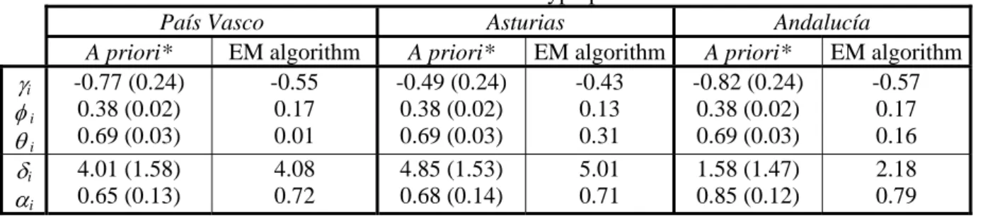
The parameters of the measurement equation (i and i) have been obtained as the regional

share in the national GAV (see table 2) using an OLS regression9. Table 2 also summarises the results for the three regions considered for the estimation process using the EM algorithm. As it can be seen, there are important differences between both sets of estimates, especially for the parameters associated to factors share in the regional production function. In particular, the EM estimates are much lower than the a priori estimates having no economic interpretation, being this one of the main disadvantages of the application of this algorithm. Last, it is important to remark that the variances of the perturbance terms of both equations have been estimated in both cases by maximum likelihood obtaining similar values.

TABLE 2

Nevertheless, to obtain estimates of the state vector (the regional manufacturing indicator), the initial values of the state vector and its associated prediction error covariance matrix are also needed. To solve the problem of the initialisation of the Kalman filter, we have followed the proposal of Harvey (1981 and 1989) and Bell and Hillmer (1991), which consists of starting the recursions from t=0 assuming that the initial values of the unobservable variable (0) are equal to zero and the prediction error covariance matrix (P0) is equal to ·I, where I is the identity matrix and the constant  has been approximated by 106 as in most empirical studies.

3.3 Validation of the results

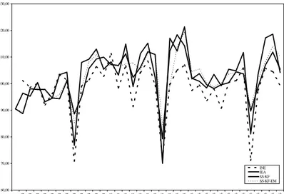
Once the hyperparameters have been estimated using the two different previously mentioned approaches (a priori estimation and EM algorithm) and the problem of initial values of the Kalman filter has been solved, it is straightforward to obtain estimates of the regional industrial production indexes10. The results obtained are presented in figures 1 to 3 where the evolution of the official

9

The value of R2 and F-test for País Vasco are 0.72 and 4.93, Asturias 0.72 and 24.88 and Andalucía 0.81 and 43.25.

10

These estimates have been obtained using SAS 6.12 software. We would like to thank Philip Israilevich for sending us part of the GAUSS code used in their computations.

(EUSTAT; SADEI and IEA), the INE (INE) and latent variable models indexes (SS-KF –state space Kalman filter using a priori estimation-, SS-KF-EM –state space Kalman filter EM algorithm estimation-) are compared. As it is shown, the results obtained with the latent variable models provide a good approximation to the direct indexes’ evolution. The comparison between results obtained using the a priori (external) estimates of the hyperparameters with the ones obtained using the EM algorithm show that for the País Vasco the second works better, for Asturias the results are better using the first, while for Andalucía there are no remarkable differences.

FIGURES 1 TO 3

The results for the pseudo-R2 have also been calculated and are shown in table 3. The results using the a priori estimates of the hyperparameters or the EM algorithm are very similar. The value for Asturias and País Vasco is very similar and close to 0.5 while the value for Andalucía is higher and near 0.7. As pseudo-R2 measures how informative the fluctuations of the national indicator are to infer the size and the direction of the regional indicator, this means that the national indicator provides more valuable information about the regional evolution in Andalucía that in the other two regions.

TABLE 3

As another way of validating these results, the MAPE between the series shown in figures 1 to 3 plus the results obtained adding one time the standard deviation of the a priori estimates of the hyperparameters (SS-KF+) and substracting one time this deviation (SS-KF-) for different time frequencies. The results based on a range of values around a priori (external) estimates permits to assess the sensibility of the indexes to hyperparameters. As it can be seen from table 4, there are no relevant differences between the results obtained using the a priori (external) estimates (SS-KF) or the “adjusted” a priori (external) estimates (SS-KF+ and SS-KF-). However, there are several cases where MAPE values are a bit lower for the second ones. In general terms, the results confirm the conclusions derived from the graphical analysis, but it should be remarked that indexes elaborated using EM estimates provide always better results at quarterly and yearly frequencies.

TABLE 4

Additionally, to analyse if the latent variable models provide more reliable indicators than the indirect method used by the INE, the above mentioned indexes have been compared for the same period (1994-96) with the official ones. The results obtained in terms of MAPE can be found in table 5. As can be seen in this table, in general the results based on latent variable models are better for the three considered regions at yearly, quarterly and monthly basis than the ones obtained using the INE method.

TABLE 5

4 Conclusions

In a previous work, Clar et al. (2000), we analysed the advantages and disadvantages of the indirect method used by the INE for measuring manufacturing quantitative indicators for the Spanish regions. The results showed that this method is only valid under certain hypothesis (among others, the similarity of the regional productive structure to the national structure, the weight of the regional manufacturing production in the national production, etc.),

For this reason, in this paper, we have estimated a latent variable model, following Israilevich and Kuttner (1993), using the Kalman filter with the aim of overcoming some of the defficiencies of the INE's method. The results obtained for the three Spanish regions where direct indicators were available show that this method overcomes some of these difficulties. These conclusions could be confirmed as more regional statistic information becomes available. In this sense, it is also important to remark that the estimates of labour and capital could be improved; the production function could be extended to consider richer specifications for technology and the possible change of factors share over time; and the dynamicity of the relationships between regional and national economic activity could be analysed in more detail.

Last, the empirical results also highlight the potentiality of the state-space modelization and the Kalman filter to analyse economic data, especially in a regional economic context. The consideration of different procedures to estimate unknown values of hyperparameters has also permit to compare their accuracy. There seems to be evidence in favour of using the EM algorithm instead of the a priori (external) estimates of some hyperparameters. However, the a priori estimates provide quite accurate results, have a clear economic interpretation and much less complexity and computational time.

5. References

Bell WR, Hillmer, SC (1991) Initializing the Kalman filter for nonstationary time series models. Journal of Time Series Analysis 4:238-300

Clar M (1998) Una anàlisi metodològica pel seguiment conjuntural de l’activitat industrial de les regions espanyoles Ph. D. Dissertation, University of Barcelona

Clar M, Ramos R, Suriñach J (1998) Potencialidad de la modelización state-space y el filtro de Kalman para el análisis regional. Una aplicación para el índice de producción industrial. University of Barcelona Working Paper E98/39

Clar M, Ramos R, Suriñach J (2000) Avantatges i inconvenients de la metodologia de l'INE per a elaborar indicadors de la producció industrial per a les regions espanyoles. Questiió 24:151-186 Dempster A, Laird N, Rubin D (1977) Maximum likelihood from incomplete data via the EM

algorithm. Journal of the Royal Statistical Society Series B 39:1-38

Griliches Z, Jorgenson DW (1966) Sources of measured productivity change: capital input. American Economic Review 56:50-61

Hackl P, Westlund AH (1996) Demand for international telecommunication: time-varying price elasticity. Journal of Econometrics 70:243-260

Harvey AC (1981) The econometric analysis of time series Oxford, Deddington

Harvey AC (1984) Dynamic models, the prediction error decomposition and state-space models. In: Hendry DF, Wallis KF (eds) Econometrics and quantitative econometrics. Basil Blackwell, Oxford

Harvey AC (1989) Forecasting, structural time series models and the Kalman filter Cambridge University Press, Cambridge

Harvey AC (1990) The econometric analysis of time series (Second edition) Phillip Allan, New York Israilevich P, Kuttner K (1993) A mixed frequency model of regional output. Journal of Regional

Science 33:321-342

Moody CE (1974) The measurement of capital services by electrical energy. Oxford Bulletin of Economics and Statistics 36:42-52

Shumway RH, Stoffer DS (1982) An approach to time series smoothing and forecasting using the EM algorithm. Journal of Time Series Analysis 3:253-264

Watson MW, Engle RF (1983) Alternative algorithms for the estimation of dynamic factor, MIMIC and varying coefficient regression. Journal of Econometrics 23:385-400

TABLES

TABLE 1. Estimates of the production function in the presence of fixed effects.

Xjt = -0.61157+0.69499LMANjt+0.38304PKMANjt j=Andalucía, Asturias, País Vasco t=1964-91

t-ratio (-2.544) (26.420) (16.355) R2=0.9422

Estimated fixed effects: Individual Andalucía=-0.21167

Asturias=0.11637 País Vasco=-0.16833

The number of observations is 238 (17 regions and 14 years). LMAN and PKMAN denote the logarithm of workers employed and private capital stock in manufacturing respectively.

TABLE 2. Estimates of the hyperparameters.

País Vasco Asturias Andalucía

A priori* EM algorithm A priori* EM algorithm A priori* EM algorithm

i  i  i -0.77 (0.24) 0.38 (0.02) 0.69 (0.03) -0.55 0.17 0.01 -0.49 (0.24) 0.38 (0.02) 0.69 (0.03) -0.43 0.13 0.31 -0.82 (0.24) 0.38 (0.02) 0.69 (0.03) -0.57 0.17 0.16 i i 4.01 (1.58) 0.65 (0.13) 4.08 0.72 4.85 (1.53) 0.68 (0.14) 5.01 0.71 1.58 (1.47) 0.85 (0.12) 2.18 0.79 * Standard errors in parentheses.

TABLE 3. Pseudo-R2 values associated to the latent variable models. 1994-96. SS-KF SS-KF-EM

País Vasco 0.50 0.47

Asturias 0.48 0.48

Andalucía 0.66 0.69

TABLE 4. MAPE values associated to the latent variable models at monthly frequency. 1994-96. SS-KF SS-KF+ SS-KF- SS-KF-EM

País Vasco 6.20% 7.33% 5.00% 3.21%

Asturias 3.10% 3.27% 3.44% 4.29%

Andalucía 4.89% 4.71% 5.25% 4.62%

TABLE 5. MAPE values associated to the INE indicators at monthly frequency. 1994-96.

FIGURES

FIGURE 1. EUSTAT, INE and latent variable indexes

FIGURE 2. SADEI, INE and latent variable indexes

FIGURE 3. IEA, INE and latent variable indexes 35,00 45,00 55,00 65,00 75,00 85,00 95,00 105,00 115,00 125,00 135,00 1/ 94 2/ 94 3/ 94 4/ 94 5/ 94 6/ 94 7/ 94 8/ 94 9/ 94 10/ 94 11/ 94 12/ 94 1/ 95 2/ 95 3/ 95 4/ 95 5/ 95 6/ 95 7/ 95 8/ 95 9/ 95 10/ 95 11/ 95 12/ 95 1/ 96 2/ 96 3/ 96 4/ 96 5/ 96 6/ 96 7/ 96 8/ 96 9/ 96 10/ 96 11/ 96 12/ 96 INE EUSTAT SS-KF SS-KF-EM 60,00 70,00 80,00 90,00 100,00 110,00 120,00 1/94 2/94 3/94 4/94 5/94 6/94 7/94 8/94 9/94 _{10/94 11/94 12/94} 1/95 2/95 3/95 4/95 5/95 6/95 7/95 8/95 9/95 _{10/95 11/95 12/95} 1/96 2/96 3/96 4/96 5/96 6/96 7/96 8/96 9/96 _{10/96 11/96 12/96} INE SADEI SS-KF SS-KF-EM 60,00 70,00 80,00 90,00 100,00 110,00 120,00 130,00 1/94 2/94 3/94 4/94 5/94 6/94 7/94 8/94 9/94 10/94 11/94 12/94 1/95 2/95 3/95 4/95 5/95 6/95 7/95 8/95 9/95 10/95 11/95 12/95 1/96 2/96 3/96 4/96 5/96 6/96 7/96 8/96 9/96 10/96 11/96 12/96 INE IEA SS-KF SS-KF-EM