Using Individualised Choice Maps to Capture the Spatial
Dimensions of Value Within Choice Experiments
Tomas Badura1,2,5 · Silvia Ferrini1,3 · Michael Burton4 · Amy Binner5 · Ian J. Bateman5
Accepted: 24 June 2019 / Published online: 1 August 2019 © The Author(s) 2019
Abstract
Understanding how the value of environmental goods and services is influenced by their location relative to where people live can help identify the economically optimal spatial distribution of conservation interventions across landscapes. However, capturing these spa-tial relationships within the confines of a stated preference study has proved challenging. We propose and implement a novel approach to incorporating space within the design and presentation of stated preference choice experiments (CE). Using an investigation of pref-erences concerning land use change in Great Britain, CE scenarios are presented through individually generated maps, tailored to each respondent’s home location. Each choice situation is generated in real time and is underpinned by spatially tailored experimental designs that reflect current British land uses and incorporate locational attributes relating to physical and administrative dimensions of space. To the best of our knowledge, this rep-resents the first CE study to integrate space into both the survey design and presentation of choice tasks in this way. Presented methodology provides means for testing how presenta-tion of spatial informapresenta-tion influence stated preferences. We contrast our spatially explicit (mapped) approach with a commonly applied tabular CE approach finding that the former exhibits a number of desirable characteristics relative to the latter.
Keywords Choice experiment · Distance decay · Economic valuation · Maps · Spatial and temporal issues · Spatial heterogeneity · Stated preferences · Survey design
* Tomas Badura [email protected]
1 Centre for Social and Economic Research on the Global Environment (CSERGE), School
of Environmental Sciences, University of East Anglia, Norwich Research Park, Norwich NR4 7TJ, UK
2 CzechGlobe – Global Change Research Institute of the Czech Academy of Sciences, Brno,
Czech Republic
3 Department of Political and International Sciences, University of Siena, Siena, Italy
4 School of Agricultural and Resource Economics, The University of Western Australia (M089), 35
Stirling Highway, Crawley, WA 6009, Australia
5 Land, Environment, Economics and Policy Institute (LEEP), University of Exeter Business School,
1 Introduction and Literature Review
Choice experiments (CEs) have been increasingly used to inform decision makers about preferences for and values regarding potential environmental change (e.g. Johnston et al.
2017). At the same time researchers have stressed the importance of ensuring the validity and reliability of elicited welfare estimates for analyses that assist policy making (John-ston et al. 2017; Desvousges et al. 2016). Substantial progress has been made to develop informative and valid CEs for environmental decision making. For example, the impacts of variation in attributes, levels, number of choice cards and order have all been extensively examined (DeShazo and Fermo 2002; Hensher et al. 2005; Day and Pinto Prades 2010; Day et al. 2012; Meyerhoff et al. 2015; Ribeiro et al. 2017), as well as information effects (Czajkowski et al. 2016b), sensitivity to scope (Czajkowski and Hanley 2009), design dimensionality, the status quo ‘bias’ of an unexpected propensity to choose the current over alternative states (Boxall et al. 2009; Oehlmann et al. 2017) or attribute non-attendance (Hussen Alemu et al. 2013; Scarpa et al. 2013). However, a topic of considerable interest concerns the capture of spatial variation in the value of environment-related goods within CE investigations of willingness to pay (WTP) for changes in the provision of such goods.
The physical characteristics of ecosystems vary across space, this affects both their capacity to produce ecosystem services and the potential for these services to generate ben-efits and value (Fisher et al. 2011; Bateman et al. 2011a, b, c). For example, water puri-fication or flood protection services benefit downstream populations while the economic benefits of pollination are confined to nearby agricultural production. Similarly, proximity to human settlements can be a major determinant of certain environment-related values— e.g. green space located close to residential areas has the potential to generate large recrea-tional benefits, whereas a physically similar green space located in remote and/or inacces-sible areas provides limited recreational benefits (Parsons 2017). Environmental policies are likely to generate spatial and temporal trade-offs in the provision of ecosystem related goods and services (Rodríguez et al. 2006; Fisher et al. 2009; Fisher and Turner 2008). Understanding spatial trade-offs between competing land uses and preferences for (poten-tial) changes is crucial for the efficient targeting of policy interventions (e.g. Bateman et al.
2011a, b, c, 2013; Fisher et al. 2011; Johnston et al. 2016).
The effects of distance upon value are long acknowledged and indeed form the basis of travel cost revealed preference modelling (Hotelling 1949; Clawson and Knetsch 1966; Bockstael and McConnel 2007). The incorporation of space within CE studies is an increasing feature of the valuation literature (e.g. Adamowicz et al. 1994; Johnston et al.
2002; Campbell et al. 2008, 2009; Brouwer et al. 2010; Schaafsma et al. 2012, 2013; Mey-erhoff 2013; Schaafsma and Brouwer 2013; Johnston and Ramachandran 2014; Czajkowski et al. 2016a; Johnston et al. 2016; Interis and Petrolia 2016; Holland and Johnston 2017; Bakhtiari et al. 2018; De Valck and Rolfe 2018; Glenk et al. 2019). Initial interest in the spatial aspects of environmental preferences within stated preference (SP) valuation stud-ies was motivated by the definition of relevant markets for aggregation of estimated values (e.g. Sutherland and Walsh 1985; Pate and Loomis 1997). In the context of CEs, initial studies included distance to the valued site, good and/or service in the attribute description (e.g. Adamowicz et al. 1994). The “distance decay” effect (Bateman et al. 2000; Loomis
2000)—the phenomenon of decreasing magnitude of elicited values with increasing dis-tance of a beneficiary to a valued site and/or good/service—has been documented by an expanding body of literature (e.g. Bateman et al. 2006; Schaafsma et al. 2012, 2013; Liekens et al. 2013). Distance decay has been shown to vary across different goods and
sites, users and non-users (e.g. Sutherland and Walsh 1985; Bateman et al. 2000, 2006; Schaafsma et al. 2013) and is influenced by the availability and proximity of substitutes (e.g. Schaafsma et al. 2013; De Valck et al. 2017). Substitutes are increasingly incorporated in CE studies—either explicitly in the study design or implicitly in the data analysis—and were shown to impact preferences for environmental changes with significant implications for value aggregation (Schaafsma et al. 2013; Jørgensen et al. 2013; Lizin et al. 2016; De Valck et al. 2017). Distance decay has been also shown to be influenced by perceptions and characteristics of the good being valued (Andrews et al. 2017). Beyond physical space, people have also been shown to have heterogeneous preferences across political bounda-ries, for example, exhibiting “premiums” for environmental goods and services delivered in the respondent’s own country of residence (Dallimer et al. 2014; Rogers and Burton
2017; Bakhtiari et al. 2018). Such ‘cultural’ preferences for the provision of environmental goods and services related to administrative, political and/or other cultural boundaries were shown to be motivated by inter alia sense of ownership, cultural identity or ethical con-cerns (e.g. Hoyos et al. 2009; Ressurreição et al. 2012; Dallimer et al. 2014; Dallimer and Strange 2015; Daw et al. 2015; Faccioli et al. 2018). Further spatial heterogeneity in prefer-ences for environmental changes have been documented, for example, related to whether the changes occur near to population centres or in remote and wild areas (Glenk and Mar-tin-Ortega 2018).
The spatial context of choices has been increasingly portrayed through maps and graph-ics (e.g. Bateman et al. 2011a, b, c; Schaafsma et al. 2012, 2013; Johnston et al. 2016; Holland and Johnston 2017). Maps and spatial information in general have been shown to influence spatial and non-spatial policy attributes as well as WTP estimates in SP studies (Johnston et al. 2002, 2016). Due to practical difficulties, these maps are rarely tailored to the location of individual respondents. Such “individualisation”, however, has been shown to be an important aid to help respondents locate themselves relative to the location of pro-posed environmental interventions and can impact on preferences and WTP estimates for such policy action (Johnston et al. 2016).
Building on the above research this paper presents a novel methodology for incor-porating spatial complexity in CE that overcomes some of the limitations of previous approaches. It explicitly incorporates two spatial attributes into the experimental design, one concerning the distance from the respondent to a ‘policy’ site at which a change occurs, and second concerning the ‘cultural’ location of the site, here proxied by whether it was located in the respondents home country or not. By manipulating the design we examine the effects of both distance and country upon preferences and values. Further, the methodology utilises a detailed spatial database of the study region to generate ‘individu-alised choice maps’, tailored to the respondent’s location. Each map is individu‘individu-alised— showing both the locations of hypothetical change and also the respondent’s home location. By automating these operations to work in real time during the CE survey tailored spatial information can be generated for each respondent. Through utilization of the spatial data-base combined with real-time programming of a site selection mechanism, data-based on spa-tially explicit experimental design, our approach addresses a gap in existing literature by allowing a wide variation of spatial attributes not only across, but also within respondents, while at the same time presenting realistic intervention locations on individualized maps. Taken together, this approach (to our knowledge) presents the most complete incorporation of space in the design and presentation of a stated preference survey to date and one that could be replicated for different contexts.
The methodology developed in this study can be utilised to elicite WTP estimates which vary across space according to the characteristics of the environment and the location of
the valuing population. The approach can also be used to test the effects of different forms of spatial detail provided to CE respondents. To demonstrate this, preferences elicited via our individualised choice maps are contrasted with those obtained from a separate sample facing the same choices but presented through the more commonly used tabular approach. Estimating mixed logit models in WTP space on data collected under these two treatments clearly shows that the approach to presenting spatial information in CE studies has an impact on stated preferences and estimated WTP values with evidence supporting mapped as opposed to tabular modes. In closing, we discuss the potential extensions of the pre-sented methodology which might help to further enhance the use of CE and SP research in supporting environmental policy formation.
2 Methodology: Survey Instrument Development and Experimental
Design
The principal objective of this research is to provide a methodology for incorporating spatial complexity within CE studies. This is achieved through an illustrative case study addressing a key and contemporary policy concern. The survey examines preferences for changes in land use from high intensity agriculture to either low intensity farming or to woodland.1 Agriculturally driven land use change is one of the major causes of environ-mental change (Foley et al. 2005; UN Environment 2019). The UK, in particular, has wit-nessed over the past half century a substantial expansion in farmland accompanied with a major increase in the intensification of agricultural production2 which has, in turn, been the major driver of biodiversity loss in the UK (Hayhow et al. 2016; Burns et al. 2016). Simul-taneously, population growth of more than 20% over this period (ONS 2015) has increased pressure upon and demand for outdoor recreational areas. The need to address biodiversity loss through the creation of new conservation sites is recognised in Government commis-sioned advice (Lawton et al. 2010) as is the importance of enhancing recreational engage-ment and environengage-mental improveengage-ments on agricultural lands. Consequently, the Govern-ment has announced its intention to alter the focus of future farm subsidies towards the provision of public goods with a principal focus upon environmental improvements (Defra
2018). However, the role of public preferences within such initiatives is not addressed. Given this, the present study also sets out to provide such advice.
2.1 The Spatial Choice Experiment 2.1.1 Valuation Scenario
The interventions broadly represent agri-environmental interventions as currently imple-mented under the Common Agricultural Policy Pillar 2. This is a pertinent and relevant
1 This survey portrayed two distinct scenarios of new forms of land use: (1) low intensity agriculture and
(2) woodland; both broadly representing interventions under agri-environmental schemes. However because the focus of this paper is on the general treatment of space in CEs, and because the end land use did not affect the general conclusions about the impact of differing treatments of space, we combine the data from the two end uses. The full results including the impact of differing end uses on WTP are provided else-where, please contact corresponding author.
2 Through dramatic changes in farming practices including increased use of chemicals the UK agriculture
focus of the study given that this is where the shift of public funding in the UK is expected in the future. The baseline and alternative end points were described using text and illus-trative photographs.3 All respondents faced two blocks of 6 choice questions—one block concerning change to low intensity agriculture and second change to woodland. The order in which respondents saw the two blocks of questions was randomised across respondents, as was the order of choice questions within each block.
Each choice question asks the respondent to choose between four options, these being the ‘opt-out’ status quo (staying with intensive agriculture at no additional cost) and three alternatives each describing the attribute levels of a site at which land use was changed to the alternative land use (either low intensity agriculture if the question was in a 6 question block featuring that land use, or to woodland if the question was in that block) at a speci-fied cost.
The survey instrument was piloted and refined over the course of 7 months through 4 pilot waves, with the final version of the survey used for data collection in the summer of 2016. Detailed in-person interviews were conducted in the first pilot wave which involved discussions on selected attributes and whether these are sufficient to describe the portrayed changes while also testing the initial preference expectations for the attributes. This was refined through successive piloting which, like the final survey were implemented online by a professional survey company.
2.1.2 Attribute Selection
A combination of literature review, current policy context, consultation with experts and piloting was employed as inputs and motivation for the attribute selection procedure. The attributes were selected to portray environmental enhancements in agricultural landscapes that were relevant for both land use change scenarios and that were able to capture spatial dimension of such changes. The selection process was intended to provide three catego-ries of attributes capturing the relevant characteristics of the land use interventions valued in the survey: (1) spatial attributes, (2) site characteristic attributes and (3) costs. Table 1
summarises these attributes and Appendix (Fig. 2) provides the visual representation and wording from the survey.
Distance and Country were selected as relevant spatial attributes that described the
location of alternatives in the choice experiment. Respondent-to-site (straight line) distance captures the expected distance decay effect and its potential heterogeneous influence on both use and non-use values (e.g. Bateman et al. 2006). Since the exact location of each respondent is not known ex-ante, the Distance attribute is included within the design as a simple two level (‘near v far’) attribute, the specification and treatment of which is dis-cussed in the next section on experimental design. The Country attribute—i.e. whether the site is in the same country of Great Britain (either Wales, Scotland or England) as the respondent’s home location—allows for testing of the impact of administrative bounda-ries. Several valuation studies have documented preferences for provision of environmental related goods in the same country as respondents are located (e.g. Dallimer et al. 2014;
3 A simple quiz followed the explanation of scenarios that tested the understanding of the main dimensions
of change [e.g. Which of the two land uses (high intensity agriculture vs. new woodland) is likely to use lower levels of chemical inputs?]. Respondents were allowed to continue with the survey only after the cor-rect answer was selected in order to ensure the comprehension of the main dimension of change presented in the survey. An option to revise previously given information was available when answering the quiz.
Rogers and Burton 2017), however only one previous study (Bakhtiari et al. 2018) exam-ined these issues while at the same time controlling for distance. The Country attribute is relevant for Great Britain given its historical and current political context, but note that the approach presented here could theoretically accommodate other administrative attributes such as counties or regions.
Three site attributes—Birds, Size and Access—provide the main descriptors of on-site scenario change. First, motivated by a vast literature on the use of birds as indicators of biodiversity (e.g. Gregory et al. 2003; Bateman et al. 2013; Harrison et al. 2014) as well as the very clear strength of preferences regarding birds in Great Britain (RSPB 2017), bird species were chosen as the major taxa used in the description of biodiversity impacts of proposed changes. Following a consultation with an expert biologist,4 the Birds attribute was chosen such that it embodied two dimensions of bird population change likely to result from different levels of conservation interventions: species abundance (i.e. number of birds of existing species in the area) and species richness (i.e. number of bird species in the area). Both dimensions were reflected in the text, labelling and pictogram5 presentation of
Table 1 Attribute levels Spatial attributes (binary)
Country (= 1) if site located in the same country as respondent (= 0) if site located in other country than respondent
Distance Distance (in miles) from the respondent’s home location to the proposed intervention site location; two levels in experimental design: less than 60 miles (near); more than 60 miles (far)
Site characteristic attributes (binary, continuous and categorical)
Access (to site) (= 1) if site will be accessible for recreation (= 0) if site is closed to the public
Size (of site) 7 ha (small)
100 ha (medium) 400 ha (large)
Birds0 Little or no increase in the number of birds and wildlife already present in the area of the site
Birds1 Some increase in the number of birds and wildlife already present in the area of the site
Birds2 Substantial increase in the number of birds and wildlife already present in the area of the site
Birds3 Substantial increase in the number of birds and wildlife already present; Some increase in the number of species in the area of the site Birds4 Substantial increase in the number of birds and wildlife already present;
Substantial increase in the number of species in the area of the site Cost attribute (continuous)
Price Increase in annual water bill per household (£15, £30, £70, £100, £150 or £200)
5 Each of the four levels were represented by corresponding number of bird pictograms. The first two levels
used the same bird species pictogram while levels three and four were represented with additional two spe-cies pictograms.
4 Gavin Siriwardena, Head of Terrestrial Ecology and Principal Ecologist at the British Trust of
attributes, and links to other wildlife in the area were explicitly mentioned (see Table 1 and Fig. 2). Three site Size attribute levels reflected the need to examine scope sensitivity in valuation exercises (see e.g. Carson and Mitchell 1993a, b; Czajkowski and Hanley 2009; Johnston et al. 2017), as well as the aim to use the estimated welfare measures for value transfers to evaluate policy interventions in GB. The Access attribute provided a simple yet effective route for separating use and non-use dimensions of value. Accessible sites yield both recreational use values and non-use values while sites without access preclude use values and allow us to inspect the pure non-use, existence value of conservation.
A cost attribute was included as a standard practice for deriving marginal WTP values for each attribute. The payment vehicle chosen was an increase in annual water bills. Given the near impossibility of avoiding payment of water bills in the UK this provides an excel-lent CE payment vehicle which mitigates against common problems of free-riding (Bate-man et al. 2002).
2.1.3 Experimental Design
Generating the experimental design for the study was complicated by the fact that the feasi-ble levels of the spatial variafeasi-bles that a respondent could see were conditional upon where they lived. In the design stage Distance to a site from the respondent’s home was defined as a binary variable: ‘near’ or ‘far’, while the Country variable was defined as ‘home country’ or ‘other country’. Respondents located close to the two borders in GB (that between Eng-land and Wales, and the border between EngEng-land and ScotEng-land) can feasibly face all four of these combinations, and hence for these respondents a design can be generated with all four elements. For those who live far (i.e. more than 60 miles) from the border, it is infeasible that they will be presented with a site that is both ‘near’ and ‘other country’ and a design is needed that excludes this combination. At the same time the model would be estimated on all respondents, irrespective of where they live. We employed the ‘model averaging’ (Rose et al. 2009) capability of Ngene software to simultaneously generate efficient designs for the two types of respondents, under the assumption that data from both will be combined within a single estimation framework, with common marginal utilities.
A Bayesian prior, D efficient design was generated using Ngene. The D efficiency crite-rion was selected, because a number of hypotheses were planned to be tested. The design was updated in a sequential manner (Scarpa et al. 2007). In the initial version of the experi-mental design the D priors were based on the expected signs of attributes (Sandor and Wedel 2001; Ferrini and Scarpa 2007). In subsequent rounds, priors were updated by esti-mated model results obtained from the waves of pilot studies. In the implementation phase (described below) respondents were given blocks of questions drawn from the appropriate design based on where they live.
2.1.4 Spatial Choice Set Generation
A key design contribution of the methodology developed in this paper is the programming of the online survey instrument to achieve real-time generation of choice sets individually tailored to the location of each respondent. This is achieved by first relating the home loca-tion provided by the respondent (in the form of their postcode) to a 2 km grid square data set of over 55 thousand cells detailing current land use for the entire area of GB (detailed in Bateman et al. 2011a, b, c, 2013; UK NEA 2011, 2014). This allowed identification of those respondents who were or were not ‘nearby’ to a country border and allocation to the
appropriate design. It was also crucial for using the database for determining locations of sites that conform to spatial attributes in given choice situations. The location of each new site was determined using programmed steps which first restricted all possible locations (i.e. all cells from the database) to the 63% of the total area of the country currently under inten-sive agricultural production. The agricultural land was identified using GIS analysis of the land use database in the design stage of the survey. A second step then used the ‘Country’ attribute to further restrict sites (i.e. 2 km grid squares from the database) to either the ‘home’ or ‘other’ country as determined by the design. Finally, the design then started searching across all remaining eligible cells (at random) until it found one with the Distance level specified in the experimental design for the given alternative and choice situation. When the site satisfying both spatial attributes was selected its location and the calculated distance was stored for analysis and display. This procedure is then repeated to generate the two other new site options which, with the no-change baseline, comprise the four options of each choice set.
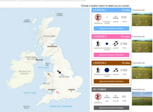
Further programming allowed the real time creation of a map, presented to the respond-ent as part of each choice set, illustrating the location of the three new land use sites and the respondents’ home (with a house symbol). The generation of each map took a fraction of a second with no distinguishable time delay for a respondent. Figure 1 and Figures 3–5
in the Appendix provide examples of this “Maps” presentation mode which embeds a con-ventional tabular summary of attribute levels for all four options which are labelled and colour coded6 to allow the respondent to readily relate these to the mapped site locations. As the Figure shows, to remind respondents of the baseline land use (intensive agriculture) and potential new land use (either low intensity agriculture or woodland), pictures previ-ously used in the scenario description were also displayed alongside each option in the tabular part of the figure. An information icon was included to provide respondents the opportunity to consult previously displayed information about each land use scenario. Each map displayed the border between each country, the country name and its capital city.7 A detailed step-by-step example choice question was provided that included instructions on how to answer the questions and/or consult previously given information.
The approach to choices set generation and presentation contrasts with conventional CE approaches in four ways. First, in a significant number of valuation studies the spatial con-text is presented in a somewhat abstract tabular format (i.e. distance only given in numeric form, with no direction information or visual representation; e.g. Adamowicz et al. 1994; Luisetti et al. 2011; Liekens et al. 2013). Second, in cases where maps are used in CE stud-ies they are rarely individualised by making each respondent’s location explicit (see John-ston et al. 2016 for individualised maps; see e.g. Schaafsma et al. 2013 for a generic map). Third, due to practical difficulties, only rarely is the choice set generated in real-time (see Bateman et al. 2016 for a revealed preference example). Fourth, by supplementing the con-ventional tabular approach with map presentation we emphasise the location, distance and directionality of proposed sites in the manner which such variables are most commonly encountered by respondents; in relation to their own location. By clarifying the substantial variation associated with each of the different choice options we bring that variation into the CE in an accessible manner which, we contend, helps facilitate the transfer of valuation
6 Colours were chosen in a manner to avoid any common colour-blindness problems.
7 This approach can readily be adapted to include further spatial or satellite data or imagery. The current
approach adopts a relatively simple and uncluttered approach to mapping intended to maximize informa-tional clarity.
findings across all feasible locations. This latter characteristic of our methodology is par-ticularly important given the policy need for value transfer information.
Our expectation is that, by mapping the spatial location of the new site options and their home, respondents will gain a superior understanding of the spatial aspects of choice options than that provided by the standard tabular approach to CE choice set presentation. Aside from the fact that online software, mobile phones and other navigation aids have greatly increased everyday usage of maps, the Maps presentation mode also provides richer spatial informa-tion (e.g. direcinforma-tion) than provided in the Tabular format. To assess the effect of this novel approach to choice set presentation, we conduct a split sample comparison of this Maps based mode of display with a separate Tabular treatment identical in all respects (including experimental design and functionality) but from which the map display was omitted, leaving just the standard tabular information used in CE studies (i.e. only the tables and photographs shown on the right side of Fig. 1, with the addition of a “country” attribute with levels Eng-land, ScotEng-land, Wales). The Tabular subsample was also given two further questions in the Map format and was asked additional questions regarding their opinions and personal prefer-ences between the two formats and how the map format influenced their responses.
2.2 Data
A nationally representative sample was recruited by a professional panel provider. In order to collect sufficient responses to estimate the Country parameter a fixed quota for responses
from England, Scotland and Wales was set at 68%, 16%, 16%, respectively; somewhat over-sampling the latter two countries (relative to their populations) in order to ensure adequate sample sizes. The responses to the final version of the survey were collected online during August and September 2016. The sample was cleaned from inattentive respondents and protest responses (see e.g. Brouwer and Martín-Ortega 2012) using standard approaches designed to avoid problems of scenario credibility failure (Powe and Bateman 2004).8
Table 2 reports selected descriptive statistics for the subsamples from each of the two treatments alongside responses to a number of key questions concerning the survey. Using a two sided t test, we found no evidence of differences in means for all variables, apart from the percentage of respondents that overall found the survey difficult which was higher for the Maps sample (p value 0.047). Similarly, Kruskal–Wallis equality-of-populations rank test showed no statistically significant differences in socio-economic characteristics between the Map and Tabular samples.
3 Modelling Responses: Theory and Methods
3.1 Random Utility Maximisation and Modelling Strategy
Discrete choice models are grounded in Random Utility Maximisation theory (McFadden
1973). This assumes that, in considering alternatives, a respondent chooses, with an unob-servable component, that option which is perceived to offer the highest level of utility (U). The utility U for a given alternative is composed of a deterministic part of utility observed by the researcher (V), which is in turn a function of an individual set of preference param-eters (β) for observable attributes (x) of the alternative, and a random part of utility (ε) as follows:
This formulation and assumptions about the distribution of the error term allows researchers to make probability statements about the choice of an alternative over a given set of other options (Train 2009).
The mixed logit (or random coefficients multinomial logit) model (McFadden and Train
2000) can closely approximate a very broad class of Random Utility models (ibid.). It is used to account for the panel structure of CE data and for preference heterogeneity across the sample. The kth-respondent’s utility from choosing alternative i in the jth choice situa-tion can be represented by:
where Xijk is the set of explanatory variables observed by the researcher (including the
attributes of the alternatives and the respondent’s characteristics), and 𝜀ijk is an error term
(1)
U = V(x, 𝛽) + 𝜀.
(2)
Uijk=Vijk+ 𝜀ijk= 𝛽k�Xijk+ 𝜀ijk
8 Protest voters were identified through a series of control questions that identified respondents who found
the survey unrealistic or who are likely to be against any governmental policy. Inattentiveness was deter-mined by identifying respondents who spent an infeasible short time answering the survey. A feasible mini-mum time limit of 6 min 45 s was identified as minimini-mum to read through the text of the survey and answer the choice questions. It was determined by in-person administered survey with a number of respondents instructed to go through the survey in fastest possible way. In total 372 respondents (14.25%) were removed for the final sample. Tests confirmed that these omissions did not materially affect the key findings of this paper.
that is assumed to be iid Gumbel distributed. 𝛽′
k represents a vector of preference
param-eters which, in the general case, are individual-specific and randomly distributed across the population or as a special case can be assumed to be fixed across respondents. One approach for selecting the appropriate “mixing” (i.e. which parameters should be modelled as random and which as fixed) is to use the Lagrange multiplier test by McFadden and Train (2000) that we used for model specification.
Income heterogeneity across the population often leads to the price parameter being modelled as a random variable. This poses difficulties in deriving WTP values from mixed logit models estimated directly in preference space. An alternative is to derive consistent WTP values as proposed by Train and Weeks (2005). Here, the price parameter is assumed to be log normally distributed and the objective is to directly estimate WTP values and their distributions. To achieve this, Eq. (2) is re-parametrized to derive the WTPs as per (3):
where 𝛽price
k is the parameter associated with the price attribute, 𝛽 non−price
k is a vector of
parameters for the non-price attributes, 𝜀ijk the error term, and 𝛾k′ the vector of WTPs for
every non-monetary attribute. This model is referred to as the mixlogit in WTP-space and is estimated using simulation methods (Train 2009). This is a convenient specification to (3)
Uijk= −𝛽kprice (
𝛽nnon−price�
𝛽kprice
Xijknon−price−Xpriceijk
) + 𝜀ijk= −𝛽pricek ( 𝛾� kX non−price ijk −X price ijk ) + 𝜀ijk
Table 2 Sample descriptive statistics
Calculated based on data from Office of National Statistics UK for year 2015 and for the same age group (18 + years old) as in the study sample
Treatment Maps Tabular Pooled Variable description
Sample size 1911 327 2238
Socio-economic variables
Gender 0.45 0.49 0.46 Portion of sample that is female (GB averagea in 2015 = 0.51)
Age 49.3 51.1 49.6 Respondent age (GB average9 in 2015 = 48.3 years)
Income (£/m) 3003 3087 3016 Total monthly household income before tax Follow up questions
Policy impact 5.6 5.5 5.6 How likely is this survey to influence policy? (10 = most likely)
Nature visits 2.5 2.6 2.5 How often you make trips to outdoor for recreation (5 = every day)
Choices difficult 2.6 2.6 2.6 How difficult it was to make CE choices? (5 = very difficult) Survey long 6.6% 4.3% 6.3% Portion of respondents finding survey overall too long Survey difficult 16.9% 12.8% 16.3% Portion of respondents finding survey overall too difficult Survey-related variables
# SQ choices 1.9 1.65 1.86 Number of times respondent chose Status Quo (out of 12 q’s) Scenario quiz 1.61 1.47 1.59 Number of attempts to answer the scenario comprehension
quiz
Choice time 21.9 22.2 21.9 Average seconds taken to answer each choice question Survey time 22.55 21.5 22.4 How many minutes it took to answer the survey
allow us to compare mean WTP values and their distributions across the Tabular and Map presentation formats.
3.2 Assessing Impact of Spatial Information
In order to assess the impact of spatial information on our model, we assume that the deter-ministic part of utility can be represented by two types of attributes; those that either are (denoted xS ) or are not (denoted xNS ) influenced by spatial information regarding the
loca-tion of sites. Examples of xS variables are likely to include both spatial attributes (Country
and Distance), while price might be a xNS variable. The utility from any spatially located
alternative can then be represented as per (4):
where 𝛽ns and 𝛽s represent associated vectors of preference parameters, sq is a dummy
vari-able that is equal to 1 for the status quo, and 𝛽0 captures preferences for that status quo
option.
We hypothesise that using different approaches to representing spatial information in a CE may have various effects upon choices. Here we have two spatial representation modes; the Maps and Tabular treatments. These could have different (or no) effect on parameters for each of the sq, xS and xNS variables. To assess these effects we combine our
theoreti-cal representation of impact that spatial information has on utility (4) with the mixed logit modelling approach estimated in WTP space (3). Assuming, for simplicity, that the price attribute is of a xNS type, we arrive at the following re-parametrisation (5):
In the results section we compare the WTP estimates ( 𝛾0
k, 𝛾
NS∶non−price
k , 𝛾
S
k ) and the price
parameter ( 𝛽price
k ) across the Tabular and Map based presentation subsamples. This
pro-vides evidence on which attributes from (4) are influenced ( xS ) by switching from the
con-ventional Tabular to the (individualised) Map presentation format, and which are not ( xNS ).
Also of interest is whether there is a difference in preferences for the change from Status Quo ( sq ) across the two treatments.
4 Results and Discussion
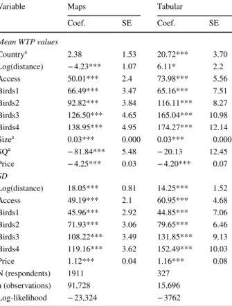
Table 3 reports results from the mixed logit models estimated in WTP-space for the Map and Tabular treatments. The Lagrange multiplier test (McFadden and Train 2000) used in selecting the randomly distributed attributes led us to treat Country, Size and SQ parame-ters as fixed, while Log(dist),9 Access, Birds1–4 and Price were specified as random, allow-ing for preference heterogeneity for these parameters across the sample population. The models assumed the Price parameter to be log-normally distributed, following common (4) U = 𝛽0sq + 𝛽nsx NS+ 𝛽 sx S+ 𝜀 (5) Uijk= −𝛽price k ( 𝛾k0sqijk+ 𝛾NS k X NS∶non−price ijk + 𝛾 s kX S∶non−price ijk −X price ijk ) + 𝜀ijk
9 Please note that following an exploratory analysis of different distance specification of the distance
vari-able, the log (distance) specification was evaluated as best performing for the analysis in terms of AIC and BIC.
applications and reflecting theoretical expectations of a negative effect of increase in price on utility, and allowed for correlation across the parameters.10 The models were estimated in Stata 13 using 3000 Halton draws for the simulation.
Table 3 reports both similarities and differences across the two treatments. Consider-ing first the similarities; consistent with empirical regularities in the literature (e.g. Cza-jkowski and Hanley 2009; Liekens et al. 2013) we find that mean WTP values for all bio-diversity coefficients (Birds1–4) are positive and increasing, with clear scope sensitivity between levels. Also as expected (e.g. Liekens et al. 2013), mean WTP for site Access is positive, suggesting some role of recreational use (or option use) value in preferences for the land use interventions. The magnitudes of the estimated standard deviations for all Bird and Access coefficients suggest high degrees of preference heterogeneity across both
Table 3 Mixed logit model of choices in WTP space for map and tabular samples (results in GBP per year)
WTP values in GBP per year (1 GBP = 1.13 EUR = 1.34 USD) ***p < 0.001; **p < 0.01; *p < 0.05
a Parameters assumed to be fixed, remaining parameters assumed to be
randomly distributed
Variable Maps Tabular
Coef. SE Coef. SE Mean WTP values Countrya 2.38 1.53 20.72*** 3.70 Log(distance) − 4.23*** 1.07 6.11* 2.2 Access 50.01*** 2.4 73.98*** 5.56 Birds1 66.49*** 3.47 65.16*** 7.51 Birds2 92.82*** 3.84 116.11*** 8.27 Birds3 126.50*** 4.65 165.04*** 10.98 Birds4 138.95*** 4.95 174.27*** 12.14 Sizea 0.03*** 0.000 0.03*** 0.000 SQa − 81.84*** 5.48 − 20.13 12.45 Price − 4.25*** 0.03 − 4.20*** 0.07 SD Log(distance) 18.05*** 0.81 14.25*** 1.52 Access 49.19*** 2.1 60.95*** 4.68 Birds1 45.96*** 2.92 44.85*** 7.06 Birds2 71.93*** 3.06 79.65*** 6.46 Birds3 108.22*** 3.49 131.85*** 9.13 Birds4 119.16*** 3.62 152.49*** 10.03 Price 1.12*** 0.04 1.16*** 0.08 N (respondents) 1911 327 n (observations) 91,728 15,696 Log-likelihood − 23,324 − 3762
10 The means and standard deviations of the price attribute were re-calculated from the original Stata
out-put, following Hole (2007). For the coefficient covariance matrices for each model please contact the lead author.
subsamples with slightly wider distributions in the Tabular sample, but in all cases the rela-tive size of mean and SD coefficients suggest a high proportion of the sample value these attribute positively. Mean WTP for the Size coefficient is positive and similar in magnitude across the two treatments; the estimates are broadly in line with results reported in Liekens et al. (2013), suggesting that a change from small (7 ha) to medium (100) and from small to large (400) site sizes portrayed in the survey equate to mean WTP of £2.8 and £11.8 per annum, respectively.
Accepting the above similarities, Table 3 also highlights a number of clear differences between the two treatments. First is a notable difference in preferences for changes from the status quo between the two subsamples. Under the Tabular presentation WTP for the
SQ is not significantly different from zero, but under the Maps treatment WTP for the SQ is significantly negative. On average then, Maps treatment respondents have a greater
preference for change from the current situation (of high intensity agriculture) than does the Tabular sample. Positive preference and WTP for a change from the status quo has been reported in similar studies concerning environmental improvements (e.g. Liekens et al. 2013; Czajkowski et al. 2016a, b; Johnston et al. 2016; an exception being Bakh-tiari et al. 2018). Multiple factors can influence the difference across the two treatments, but we believe that the main reason might be that the increased spatial detail provided by individualised choice maps makes the intervention scenario more realistic through portrayal of its specific locations at a given choice map. This, we believe, made the envi-ronmental improvements to high intensity agriculture more desired by the respondents relative to the Tabular format.
The major differences between the WTP results obtained from the two treatments are, as expected, concerning the two spatial attributes; Country and Log(dist). When faced with the Maps treatment the majority of our sample tend to care more about the distance attribute and on average disregard whether the intervention site is in the same country as they are. The opposite is true for the Tabular presentation—on average these respondents prefer the site being in the country they reside in and less pay attention to distance than those in the Maps sample. These differences show that the level of spatial detail given in the CE has significant impact on how respondents view spatial attrib-utes of environmental change. In particular, the respondents faced with the Tabular for-mat favour sites that were located in the country they live in; a similar observation can be seen in some existing CE research (e.g. Dallimer et al. 2014; Rogers and Burton
2017), including the study by Bakhtiari et al. (2018) who also control for distance while examining country effects. However, this effect was not significant for the Maps sub-sample. The difference in the significance of the country attribute across the two treat-ments might be influenced by the fact that the attribute is implicit in the Map format, expressed by the border lines and country names on the map. Country was explicit in the attribute tables in the Tabular format. This could have increased respondents’ atten-tiveness to the attribute and made the country motivation for choice of interventions’ location more pronounced.
The differences seen across the two formats in terms of the two spatial attributes and the SQ suggest complex effects of spatial information on choices. In particular, at the mean of WTP distributions only the Maps treatment shows distance decay (i.e. negative sign of the distance attribute) which we would expect from the published literature (e.g. Bateman et al. 2006; Liekens et al. 2013; Bakhtiari et al. 2018). In contrast, the WTP distribution for distance in the Tabular sample shows a counter-intuitive positive mean value, however note the large estimated standard deviations across both subsamples which shows that a great number of respondents exhibit distance decay in the Tabular
sample too while some respondents in the Maps format have a positive preference for distance.11,12 The significant preference heterogeneity could be related to both use and non-use values: the motivation for distance decay effects for non-use values is mixed (e.g. Glenk et al. 2019). We speculate that, on average, respondents presented with the Maps could have cared about the distance as much as it cancelled any effect of the coun-try attribute seen in the Tabular format while, in turn, the Tabular sample seems to have been influenced in their choices by the country attribute even to the extent that distant locations could be preferred when in the respondent’s country. This assertion is in line with previously mentioned fact that the country attribute was more pronounced in the Tabular format, but as well that distance is more explicit (i.e. visible) in the Maps for-mat. Further, the treatment effect on the spatial attributes could have been linked to the observed difference for the SQ discussed previously. The SQ captures the average effect on utility of all factors that are not included in the model that influence choices between intervention alternatives and the status quo. This could include, for example, scenario credibility mentioned above, but also the effect of each of the choice set formats. While beyond the scope of this paper, further analyses show that the three attributes, which differ most across the two treatment (i.e. SQ, country, distance), vary across individual countries’ respondents, suggesting a complex interplay of inter alia respondent’s cultural and spatial preferences, scenario credibility and framing of the choice. A number of pre-vious studies indeed showed that framing of a valuation scenario can have an effect on how distance decay differ in statistical significance or magnitude, for example, across dif-ferent goods or attributes (Pate and Loomis 1997; Concu 2007; Rolfe and Windle 2012; Johnston and Ramachandran 2014) or number of alternatives (Schaafsma and Brouwer
2013) which can also relate to the observed differences across the two treatments. Fur-thermore, although substitutes were not explicitly incorporated into the survey design nor into the presentation of choices, the individualised choice maps implicitly reflected also availability of substitutes and hence might have influenced elicited preferences dif-ferently across the two treatments. Notwithstanding the reasons for the differences seen across the two treatments, our results clearly suggest that the effect of administrative boundaries and distance on respondents’ choices is influenced by the format of a choice situation and the spatial information given to them.
Finally, use value might also play a role in how presentation of spatial information on individualised choice maps relative to Tabular format impacts on preferences for envi-ronmental change. The Tabular sample showed higher mean WTP (and larger standard deviation) estimates for the Access attribute and the two highest levels of biodiversity. It is likely that these might be related to potential use value of biodiversity through, for
11 Differences preferences for spatial attributes and the status quo are also observed in an additional
analy-sis of responses to the first choice questions faced by the two subsamples (see Appendix Table 4); first responses in stated preference data being of particular relevance in terms of their heightened incentive com-patibility relative to subsequent responses (Bateman et al. 2008, 2009; Carson and Groves 2007). Also note that similar results were also seen in a within respondent analysis of the repeated choice questions that the Tabular sample answered in both formats. The results are available at request from the corresponding author.
12 The large standard deviations estimated across both subsamples suggest that some respondents preferred
sites being further away from their residence. This might be related to unobservable motivations, for exam-ple, belief that biodiversity should be restored away from major populations; such findings could be seen in Glenk and Martin-Ortega (2018). Similarly Rolfe and Windle (2012) found positive effect of distance of some residents of Australia for the Great Barrier Reef, suggesting that distance decay might be of limited effect for some environmental assets.
example, recreation. Our results in this sense seem to be broadly in line with research by Johnston et al. (2016) and we agree with them13 that the use of individualised maps might make respondents more aware of the distances to sites; an argument that seems strengthened by the lack of difference across samples for non-spatial related attributes such as Price and site Size.
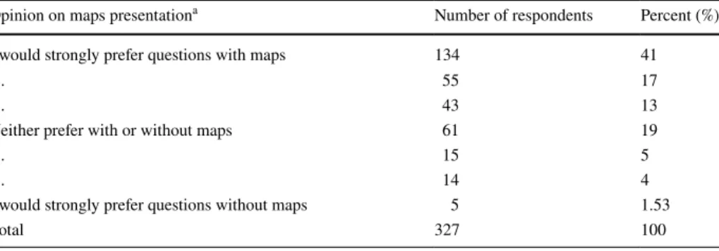
We asked the Tabular subsample that faced both modes of presentations a number of control questions regarding their thoughts on the difference between the two formats. 71% of the respondents faced with both formats indicated that they would prefer to see ques-tions with Maps and only 10.5% respondents preferred choices in Tabular format only (see Appendix Table 5). However, the map format is perceived more difficult in overall (see Table 2) which might be the necessary price to pay for more realistic choices that are likely to elicit robust policy-relevant information. The increased reported difficulty in answering the map format might be precisely due to more reflective (and hence more realistic) deci-sion process. This issue will be explored by attribute non-attendance analysis in our further work.
5 Conclusions: CE Survey Design for Spatial Preferences
This paper presents a novel approach for spatially-relevant choice experiments applied to a case study assessing preferences for land use change interventions in high intensity agricultural landscapes in Great Britain. It presents a survey instrument that incorpo-rated spatial dimensions of choice in different stages of the CE survey development. It explicitly included two spatial attributes in the experimental design—one concerning distance and the second administrative boundaries. Choice set options were generated by further taking into account current land use and the respondent’s location. Choice sets were presented to respondents through the real-time generation of individualised choice maps encompassing all of the above spatial information including where each site is, as well as where the respondent is located on a map. To our knowledge this is the first time that a CE study has incorporated these multiple dimensions into the design and display of choice sets and thereby into derived values. This approach could be adapted to other contexts (including Contingent Valuation research) to elicit spa-tially relevant preferences, derive value transfer functions and test different modes of presenting spatial information to respondents. Indeed, given that the underlying func-tionality is independent from the way the choice set is presented, this methodology is particularly well positioned to test the impacts of spatial information on WTP esti-mates. The application of the methodology presented in this paper allowed us to high-light various effects that the presentation of spatial information in CE (and perhaps SP more generally) has on stated preferences for environmental interventions. As per Johnston et al. (2016), we show that more detailed spatial information impacts on a subset of attributes and related WTP estimates; and that spatial aspects of choice can influence non-spatial attributes (Johnston et al. 2002). We note, however, that the con-figuration of the maps format on the screen makes the spatial aspect of choice more
13 Note that Johnston et al. (2016) compare individualised maps against generic maps while we compare
individualised maps against tabular format of a choice set. Nevertheless, we believe that considering gen-eralised case of a more detailed spatial information against a less detailed one in the context of CEs, our results are broadly in line.
salient than other attributes, which might have also influenced the effects of the maps format on the spatial attributes we see in our results.14 The increased salience of spa-tial attributes does not come at the expense of losing reliability of other important and theoretically established aspects of eliciting preferences, such as sensitivity to scope, while at the same time increasing the credibility and realism of the valuation scenario (through use of the spatial database). Our results also suggest that presenting choice sets on individualised choice maps is a more suitable format to portray choice tasks for (implicitly) spatial environmental changes rather than attribute tables only. The Maps format induced choices more strongly conforming to empirical regularities in the literature regarding presence of distance decay effect and lesser use of heuristics (i.e. Country attribute). Further, the Maps format provide richer spatial information to respondents which is likely to lead to better informed choices than in the Tabular for-mat. Maps are the most common wayfinding support tools (Klippel et al. 2010) and are now in common use in online software and mobile phones (e.g. Google Maps, Apple maps) which testifies to their usefulness for portraying spatially relevant choices in CEs, rather than through a Tabular format only. Additional control questions related to respondents’ opinion on the (difference between) the two presentation modes seem to confirm this assertion. However, our results clearly suggest that the effect of admin-istrative boundaries and distance decay should be further explored in light of different formats of choice situations and the spatial information given to respondents. More exact comparisons of preferences across the treatments could be employed, for exam-ple, through sample matching techniques (e.g. Liebe et al. 2015). More generally, how-ever, examining the effects of space on choices in stated preference studies requires further effort that looks at an interplay between inter alia presentation of space in the surveys, cognitive demands on respondents and scenario credibility. The presented methodology enables coherent examination of these issues.
The methodology has potential to be expanded to consider wider spatial complexi-ties. More sophisticated incorporation of distance in the experimental design15 and politi-cal jurisdictions, administrative or cultural boundaries in the experimental design could readily be envisaged, as can more advanced treatment of distance in the data analysis (e.g. Andrews et al. 2017; Holland and Johnston 2017). Similarly the resolution of the case study map, while acceptable for a national level study, remains too coarse for local level value elicitation. Switching between national and local levels via a mapping interface incorporat-ing a zoomincorporat-ing functionality would further enhance the usefulness of this approach. More fundamentally, given the clear impact on preferences of substitutes (e.g. De Valck et al.
2017; Schaafsma et al. 2013; Schaafsma and Brouwer 2013) a mapping approach seems an ideal vehicle for conveying substitute availability and this is an ongoing focus of our research.
Research concerning the incorporation of spatial and related aspects of the environ-ment within CE exercises is growing and is of increasing policy relevance and use (Natu-ral Capital Committee 2015). The present study examines how these aspects can be both
15 Note, however, that while the two levels of the distance attribute was featured in the experimental
design, respondents were faced with a high variability in the actual distance to intervention sites due to ran-dom element in site choice as explained in the section “Spatial choice set generation”.
14 While this requires further testing (by, for example, making other attributes more prominent in the
choice set presentation), it is likely that the spatial attribute salience is not the only factor at play as the Maps format also seems to impact on non-spatial attributes.
incorporated within study designs and more effectively presented to survey respondents. While the initial time and resource requirement for the development of the approach was considerable especially in terms of real-time selection and projection of the locations on the choice map,16 which indeed needs to be weighted against the particular needs of a given SP study (Johnston et al. 2016), we believe that it can be relatively easily main-streamed into SP studies in the future. In a world of increased environmental pressures (e.g. Millennium Ecosystem Assessment 2005; Rockström et al. 2009; Butchart et al. 2010; Lenzen et al. 2012; Pimm et al. 2014), relevant and reliable valuation research is increas-ingly required for ecosystem management and investment decision making (Bateman et al.
2011a, b, c; Guerry et al. 2015). The more that such research can incorporate the reali-ties and complexireali-ties of the natural environment the better it will be able to contribute to improvements in such decisions.
Acknowledgements We are grateful to three anonymous referees and the editors for excellent insights and comments that greatly helped to improve the manuscript. We would like to also express gratitude for the multiple comments provided on previous drafts of the paper presented at EAERE, ICMC, envecon and bio-econ conferences as well as at the PhD colloquium organised by Prof. David Maddison from University of Birmingham. Tomas Badura would like thank his supervisors for guidance and support and to acknowledge Zuckerman studentship funding from School of Environmental Sciences at the University of East Anglia which supported his PhD research. Ian J. Bateman and Amy Binner would like to acknowledge funding from South West Partnership for Environment and Economic Prosperity (SWEEP) (Ref. NE/P004970/1; NERC Project code: NE/P011217/1).
Open Access This article is distributed under the terms of the Creative Commons Attribution 4.0 Interna-tional License (http://creat iveco mmons .org/licen ses/by/4.0/), which permits unrestricted use, distribution, and reproduction in any medium, provided you give appropriate credit to the original author(s) and the source, provide a link to the Creative Commons license, and indicate if changes were made.
Appendix
See Figs. 2–5 and Tables 4 and 5.
The two models in Table 4 below were estimated using two conditional logit models (McFadden 1973), on first choices only, for Tabular and Maps subsamples. Note that the choices are independent and given the randomisation of task orders, the models were esti-mated on full design and hence present a valid dataset for the present analysis. Further, the first question in a CE exercise has a number of convenient properties, particularly their heightened incentive compatibility relative to subsequent responses (Bateman et al. 2008,
2009; Carson and Groves 2007; Scheufele and Bennett 2013).
16 In essence, the individualised choice map functionality was developed in two steps. In the first one, we
used an MS Excel table of the cells available for interventions (with associated coordinates) together with developed functionality of the cell selection as described in Sect. 2.1.4. Second step was to program this functionality and to project the selected cells and respondent’s location on given map picture. In the context of currently available survey interface technology we are aware of, we believe that the higher costs would be required in terms of the second step. However, note that in our case respondent and intervention loca-tions were projected on a map figure, not using any (e.g. GIS) map interface which required relatively sim-ple programming. We hope to provide a more detailed how-to publication on the matter in the future.
Fig. 2 Presentation of attributes levels in the survey
References
Adamowicz W, Louviere J, Williams M (1994) Combining revealed and stated preference methods for valuing environmental amenities. J Environ Econ Manag 26(3):271–292. https ://doi.org/10.1006/ jeem.1994.1017
Alemu MH, Mørkbak MR, Olsen SB, Jensen CL (2013) Attending to the reasons for attribute non-attend-ance in choice experiments. Environ Resour Econ 54(3):333–359. https ://doi.org/10.1007/s1064 0-012-9597-8
Andrews B, Ferrini S, Bateman I (2017) Good parks–bad parks: the influence of perceptions of location on WTP and preference motives for urban parks. J Environ Econ Policy 6(2):204–224. https ://doi. org/10.1080/21606 544.2016.12685 43
Bakhtiari F, Jacobsen JB, Thorsen BJ, Lundhede TH, Strange N, Boman M (2018) Disentangling distance and country effects on the value of conservation across national borders. Ecol Econ 147:11–20. https ://doi.org/10.1016/J.ECOLE CON.2017.12.019
Table 4 Conditional logit model estimated on first choices only
***p < 0.001; **p < 0.01; *p < 0.05
Variable Maps Tabular
Coef. SE Coef. SE Country 0.15* (0.07) 0.34* (0.17) Log(distance) − 0.15*** (0.04) 0.01 (0.10) Access 0.53*** (0.06) 0.58*** (0.14) Birds1 0.40*** (0.10) 0.54* (0.26) Birds2 0.63*** (0.10) 0.71** (0.26) Birds3 0.77*** (0.10) 1.01*** (0.26) Birds4 1.00*** (0.10) 1.17*** (0.26) Size 0.00*** (0.00) 0.00 (0.00) SQ − 1.09*** (0.25) − 0.05 (0.61) Price − 0.01*** (0.00) − 0.01*** (0.00) N (respondents) 1911 327 n (observations) 7644 1308 Log-likelihood 2249.15 − 383.434
Table 5 Respondents’ opinion on map versus tabular presentation
a The exact phrasing of the question was as follows: “If you were to have to answer more questions like
those about the sites for land use changes, would you prefer them to have maps or not have maps?”
Opinion on maps presentationa Number of respondents Percent (%)
I would strongly prefer questions with maps 134 41
… 55 17
… 43 13
Neither prefer with or without maps 61 19
… 15 5
… 14 4
I would strongly prefer questions without maps 5 1.53
Bateman IJ, Langford IH, Nishikawa N, Lake I (2000) The Axford debate revisited: a case study illustrating different approaches to the aggregation of benefits data. J Environ Plan Manag 43(2):291–302. https :// doi.org/10.1080/09640 56001 0720
Bateman IJ, Carson RT, Day B, Hanemann WM, Hanley N, Hett T, Jones-Lee M, Loomes G, Mourato S, Özdemiroğlu E, Pearce DW, Sugden R, Swanson J (2002) Economic valuation with stated preference techniques: a manual. Edward Elgar Publishing, Cheltenham
Bateman IJ, Day BH, Georgiou S, Lake I (2006) The aggregation of environmental benefit values: welfare measures, distance decay and total WTP. Ecol Econ 60(2):450–460. https ://doi.org/10.1016/j.ecole con.2006.04.003
Bateman IJ, Burgess D, Hutchinson WG, Matthews DI (2008) Contrasting NOAA guidelines with learn-ing design contlearn-ingent valuation (LDCV): preference learnlearn-ing versus coherent arbitrariness. J Environ Econ Manag 55:127–141. https ://doi.org/10.1016/j.jeem.2007.08.003
Bateman IJ, Day BH, Dupont D, Georgiou S (2009) Procedural invariance testing of the one-and-one-half-bound dichotomous choice elicitation method. Rev Econ Stat 91(4):806–820. https ://doi.org/10.1162/ rest.91.4.806
Bateman IJ, Mace GM, Fezzi C, Atkinson G, Turner K (2011a) Economic analysis for ecosystem service assessments. Environ Resour Econ 48(2):177–218. https ://doi.org/10.1007/s1064 0-010-9418-x
Bateman IJ, Abson D, Andrews B, Crowe A, Darnell A, Dugdale S, Fezzi C, Foden J, Haines-Young R, Hulme M, Munday P, Pascual U, Paterson J, Perino G, Sen A, Siriwardena G, Termansen M (2011b) Valuing changes in ecosystem services : scenario analyses. UK National Ecosystem Assessment Tech-nical Report, pp 1265–1308. Retrieved from http://uknea .unep-wcmc.org/. Accessed 13 Dec 2018 Bateman IJ, Brouwer R, Ferrini S, Schaafsma M, Barton DN, Dubgaard A, Hasler B, Hime S, Liekens
I, Navrud S, De Nocker L, Ščeponavičiūtė R, Semėnienė D (2011c) Making benefit transfers work: deriving and testing principles for value transfers for similar and dissimilar sites using a case study of the non-market benefits of water quality improvements across Europe. Environ Resour Econ 50(3):356–387. https ://doi.org/10.1007/s1064 0-011-9476-8
Bateman IJ, Harwood A, Mace GM, Watson R, Abson DJ, Andrews B, Binner A, Crowe A, Day BH, Dug-dale S, Fezzi C, Foden J, Haines-Young R, Hulme M, Kontoleon A, Lovett AA, Munday P, Pascual U, Paterson J, Perino G, Sen A, Siriwardena G, van Soest D, Termansen M (2013) Bringing ecosystem services into economic decision making: land use in the UK. Science 341(6141):45–50. https ://doi. org/10.1126/scien ce.12343 79
Bateman IJ, Agarwala M, Binner A, Coombes E, Day BH, Ferrini S, Fezzi C, Hutchins M, Lovett AA, Posen P (2016) Spatially explicit integrated modeling and economic valuation of climate change induced land use change and its indirect effects. J Environ Manag 181:172–184. https ://doi.org/10.1016/j. jenvm an.2016.06.020
Bockstael NE, McConnel KE (2007) Environmental and resource valuation with revealed preferences, vol 7. Springer, Dordrecht. https ://doi.org/10.1007/978-1-4020-5318-4
Boxall P, Adamowicz WL, Moon A (2009) Complexity in choice experiments: choice of the status quo alternative and implications for welfare measurement. Aust J Agric Resour Econ 53(4):503–519.
https ://doi.org/10.1111/j.1467-8489.2009.00469 .x
Brouwer R, Martín-Ortega J (2012) Modeling self-censoring of polluter pays protest votes in stated prefer-ence research to support resource damage estimations in environmental liability. Resour Energy Econ 34(1):151–166. https ://doi.org/10.1016/j.resen eeco.2011.05.001
Brouwer R, Martin-Ortega J, Berbel J (2010) Spatial preference heterogeneity: a choice experiment. Land Econ 86(3):552–568. https ://doi.org/10.3368/le.86.3.552
Burns F, Eaton MA, Barlow KE, Beckmann BC, Brereton T, Brooks DR et al (2016) Agricultural man-agement and climatic change are the major drivers of biodiversity change in the UK. PLoS ONE 11(3):e0151595. https ://doi.org/10.1371/journ al.pone.01515 95
Butchart SHM, Walpole M, Collen B, van Strien A, Scharlemann JPW, Almond REA et al (2010) Global biodiversity: indicators of recent declines. SOM. Science (New York, NY) 328(5982):1164–1168.
https ://doi.org/10.1126/scien ce.11875 12
Campbell D, Scarpa R, Hutchinson WG (2008) Assessing the spatial dependence of welfare estimates obtained from discrete choice experiments. Lett Spat Resour Sci 1(2–3):117–126. https ://doi. org/10.1007/s1207 6-008-0012-6
Campbell D, Hutchinson WG, Scarpa R (2009) Using choice experiments to explore the spatial distribution of willingness to pay for rural landscape improvements. Environ Plan A 41(1):97–111. https ://doi. org/10.1068/a4038
Carson RT, Groves T (2007) Incentive and informational properties of preference questions. Environ Resour Econ 37(1):181–210. https ://doi.org/10.1007/s1064 0-007-9124-5