INFLUENCE OF THE REPRESENTATIVENESS OF REFERENCE WEATHER
DATA IN MULTI-OBJECTIVE OPTIMIZATION OF BUILDING
REFURBISHMENT
Giovanni Pernigotto
1, Alessandro Prada
2, Francesca Cappelletti
3, Andrea Gasparella
21
University of Padova, Department of Management and Engineering, Vicenza, Italy
2Free University of Bozen-Bolzano, Faculty of Science and Technology, Bolzano, Italy
3IUAV of Venezia, Dep. of Design and Planning in Complex Environments, Venice, Italy
ABSTRACT
Energy saving measures properly applied to the existing building stock can bring noticeable savings. In particular, optimal cost-effective solutions can be found through multi-objective optimization techniques, such as those based on genetic algorithms (GA), coupled with building energy simulation (BES). Although the robustness of GA multi-objective optimizations to the quality of the inputs is discussed in the literature, the role of the weather data file is not investigated in detail. For this reason, this work analysed the extent to which the method adopted for the development of reference weather data for BES can affect the optimal solutions. Considering a group of simplified building configurations and the location of Trento, Italy, many multi-objective optimizations are performed. The results show changes to both Pareto fronts and optimal retrofit solutions.
INTRODUCTION
The European Commission suggested the renovation of existing buildings into nearly zero-energy buildings through the definition of cost-optimal levels into the framework of building energy retrofitting (European Commission, 2010 and 2012). Among all possible energy saving measures (ESMs), the one that optimizes some competitive goals - such as the contemporaneous minimization of net present value (NPV) and primary energy (EP), should be chosen. For this reason, multi-objective optimization and BES can help to determine a set of equivalent optimal solutions, the so-called Pareto front. In particular, among the different alternative strategies, such as those described by Evins (2013), the evolutionary optimization approaches - and especially the genetic algorithms, have become more and more popular (Penna et al., 2015).
When dealing with imprecise input data, sensitivity issues can undermine the suitability of multi-objective optimization in finding cost optimal solutions. In this regard, while GA robustness to algorithm parameters has been widely investigated (Wright and Alajmi, 2005; Ihm and Krarti, 2012), the robustness to suboptimal inputs needs to be further discussed. In this context, reliable building simulation results depend also on the
representativeness of weather inputs, which can be sources of external scenario uncertainties (Hopfe and Hensen, 2011). In fact, both length of the multi-year weather data series (Prada et al., 2014) and methodology used for the typical month selection largely influence the results of the reference year development process (Pernigotto et al., 2014a; Pernigotto et al., 2014b). Consequently, the cost optimal identification through GA optimization could be influenced as well and the findings could lack robustness to climate changes.
The aim of this work is to investigate the extent to which the weather data used for BES can affect the robustness of GA approach for multi-objective optimization and the identified optimal solutions. In this way, it has been possible to assess the sensitivity of the optimization method to an uncertain and suboptimal input such as the typical climatic file, which can be developed according to different approaches from the same sets of raw weather data.
METHODS
Several multi-objective optimizations have been carried out with different reference years, developed according to the methods described in (Pernigotto et
al., 2014b) from a set of hourly weather data series
collected in the meteorological station of Trento, northern Italy. Various building configurations have been analysed to achieve results suitable to make generalization.
The implemented Genetic Algorithm
The choice of optimal trade-off between EP and NPV is based on the domination of a general solution X over a solution Y. According to Pareto, X dominates
Y if the following conditions are both true:
the solution X is no worse than Y in all objectives;
the solution X is strictly better than Y in at least one objective.
Thus, passing from X to Y, an improvement for some objectives, without worsening the other ones, is supposed. When an objective cannot improve without making worse the others, an “Optimum of Pareto” is found. The two steps of the optimization procedure are therefore: (a) the definition of Pareto front and (b) the selection of a trade-off solution among those belonging to Pareto front.
For the multi-objective optimization of building retrofits, a GA is implemented in Matlab®. The Matlab® fitness function used in the analysis launches BES (TRNSYS BES, in this case), reads
BES output file and post-processes the simulation
results. The code computes the NPV by means of the method proposed by the technical standard EN ISO 15459:2009 (CEN, 2009) and returns the two objectives to the genetic algorithm. In particular,
NPV and EP for space-heating (EPh) are chosen as
goals for the multi-objective optimization.
The genetic algorithm chosen in this work is Elitist Non-dominated Sorting Genetic Algorithm, NSGA-II (Deb, 2002), identified because of its better performance with respect to other GA algorithms (Brownlee et al., 2011; Evins, 2013). Moreover, it has been modified with customized sampling, crossover, mutation and selection procedures. All these modifications, together with population size and crossover fraction, are adopted with the purpose of further increasing the genetic algorithm performances (Penna et al., 2015). In the first step, the initial population, to which the genetic algorithm optimization is closely related, is selected. The Sobol sequence sampling is chosen since it produces uniform samples for high population sizes (Saltelli et
al., 2004; Burhenne et al., 2011) and reduces the risk
of oversampling. Moreover, the random starting point in Sobol sequence is obtained through a pseudo random generator (Matsumoto and Nishimura, 1998). Once the fitness function is evaluated, the genetic algorithm proceeds with the selection of the best individuals (i.e., the “parents” for the next generation). In this study, the “Tournament Selection Without Replacement” (Goldberg et al., 1989; Goldberg and Deb, 1991) has been adopted: a short list of four eligible parents are randomly chosen and, among them, the best individual is set to be a parent. Then, the genetic characteristics of both parents are combined, giving rise to the new generation. Children are a random (Matsumoto and Nishimura, 1998) arithmetic mean of two parents always feasible with respect to the bounds (Burjorjee, 2013). The adopted crossover fraction - i.e., the fraction of the next generation that crosses over, is set to 0.8. The remaining individuals in the next generation come from population mutation, randomly applied by means of Mersenne-Twister pseudo random generator (Matsumoto and Nishimura, 1998). Specifically, a gene is randomly selected and replaced by a random value from a uniform distribution that meets the gene range.
The convergence criterion is based on the crowding distance, i.e., the closeness of an individual to its neighbours (Deb, 2002). Specifically, multiple runs of the algorithm are performed until a change of 10-4 is found for the crowding distance between two consecutive generations (Jena et al., 2013). The final population contains the optimal solutions.
Building case-studies
With the purpose of ensuring the result generalization, three typologies of building are simulated: semi-detached houses (S/V = 0.97 m-1), penthouses (S/V = 0.63 m-1) and intermediate flats in multi-story buildings (S/V = 0.3 m-1), obtained by imposing an adiabatic boundary condition whenever the envelope structures are adjacent to other apartments (Figure 1). Each building has 100 m2 of floor surface, 3 m of internal height and façades oriented towards the main cardinal directions. If not adiabatic, the envelope surfaces are directly exposed to the external environment, without thermal contact with the ground for the floor of the semi-detached house. The considered configurations have windows only in one façade (East or South), which is also in front of the adiabatic vertical wall adjacent to other buildings. The window to floor ratio is equal to 0.144.
Figure 1 - Test cases used in robustness analysis Table 1 Building characteristics Opaque Envelope Windows Infiltration Rate d=0.20 m Glazing: Single-pane Intermediate flat λ=0.25 W m-1K-1 Ugl 5.69 0.06 ACH [W m-2 K-1] R=0.80 m2K W-1 SHGC 0.81 Semi-detached house κ=150 kJ m-2K-1 Frame: Standard timber 0.13 ACH ρ=893 kg m-3 Ufr 3.20 Penthouse [W m-2 K-1] c=840 J kg-1K-1 A fr/Awin 19.9 0.20 ACH
The thermal transmittances of opaque and transparent components have the typical values of the Italian building stock built before the first Italian energy saving law, law number 373 of 1976 (Table 1). The opaque envelope is a simplified massive structure with a clay-block and the glazing system includes a single-pane glass and a standard timber frame, modelled with LBNL Window 6.3. The linear thermal transmittances of thermal bridges are computed according to EN ISO 10211:2007 (CEN,
2007a) by means of LBNL THERM 6.3. The infiltration rates (Table 1) are estimated according to EN 12207:1999 (CEN, 1999) and EN 15242:2007 (CEN, 2007b), considering a reference air tightness
n50 of 7 air changes per hour (ACH). As regards the
system typically found in buildings built up to 1970s and not yet renovated, a standard boiler coupled with radiators and ON-OFF system regulation are considered.
Weather data
Representative weather information is essential for reliable building energy performance analyses. In particular, a reference year should be able to characterize the climatic conditions typical for the entire life cycle of the building. In the literature, many approaches can be found for the elaboration of the reference year, with results characterized by different levels of representativeness in the different climates (Pernigotto et al., 2014b). In this work, it has been verified how the variability of reference weather file may affect the choice of optimal retrofit solutions for the city of Trento, North of Italy (Köppen classification: Cfa; ASHRAE 169/2006 classification: 4A). Six reference years are developed starting from an historic series of 10 years, according to the following methods: (M1) EN ISO 15927-4 (CEN, 2005), (M2) Wilcox and Marion’s method (2008), (M3) the method by Pissimanis et al. (1988) and the three ones described in (Pernigotto et al., 2014b) - (M4) the minimum Finkelstein–Schafer statistic, FS, (M5) Best rank I and (M6) Best rank II. These methods differ from each other because in the same historic series of 10 years they lead to select different representative months for the reference year. The different choice of representative months brings differences in Heating Degree-Days calculated with respect to a base temperature of 18 °C (HDD18)
and in daily average global solar irradiation on horizontal surface (Isol), as shown in Table 2. In
particular, the maximum HDD18, obtained from the
method M6, Best rank II, is 2504 K d and the minimum HDD18, arising from the method M2 by
Wilcox and Marion, is 2330 K d.
Table 2
Heating Degree-Days and daily average global solar irradiation on horizontal surface obtained with different methods for the reference year development
Method HDD18 [K d] Isol [MJ m-2 d-1] M1 2499 7.98 M2 2330 7.65 M3 2496 7.27 M4 2448 7.70 M5 2484 7.50 M6 2504 7.49
Energy saving measures and economic analysis In the multi-objective optimizations, six different types of ESMs, representative of the most common
solutions adopted by designers to reduce EPh, are
evaluated (Penna et al., 2015; Prada et al., 2014):
an additional insulating layer of extruded polystyrene with a thermal conductivity of 0.04 W m-1 K-1 and thickness ranging from 0.01 to 0.20 m (with a step of 0.01 m), changed independently for the external surface of non-adiabatic walls, ceiling (only for semi-detached houses and penthouses) and floor (only for semi-detached houses);
replacement of current windows with high performance frames with Ufr = 1.2 W m-2 K-1 and
glazings (i.e., double, D, or triple, T, glazings – respectively with Ugl ≈ 1.1 W m-2 K-1 and Ugl ≈
0.6 W m-2 K-1, and either high, H, or low, L, solar heat gain coefficients of about 0.6 and 0.35, respectively);
replacement of existing boiler (STD) with either modulating (MOD) or condensing boiler (COND). In both cases the new boiler is also equipped with an external climatic adjustment in order to vary the supply temperature as a function of the external air temperature;
adding a mechanical ventilation (MVS) with heat recovery system.
Some other improvements are associated with the proposed measures. The addition of the external insulation mitigates the thermal bridges: thus, their linear thermal transmittance is recalculated and used in simulations. The windows replacements greatly increase air tightness and, thus, a reduction of 50 % is applied to the building infiltration rate. As a whole, the combinations of all possible alternative ESMs can be very high: in case of semi-detached houses, for example, more than 275 000 solutions need to be calculated in order to find the optimal one and this makes necessary the adoption of advanced multi-objective optimization techniques, such as the GA of the current research.
The prices adopted for the different ESMs have been taken from the official regional price list and the energy source prices are extracted from the database of the national authority of gas and electricity (Penna
et al. 2015; Prada et al., 2014). For the cost-optimal
analysis the NPV has been computed as suggested by the regulation EU 244/2012 (European Commission, 2012). The investment analysis is 30-year long and includes the initial investment cost, the annual running costs (composed by energy and maintenance costs), the replacement cost due to periodic substitution of building elements and the residual value for the equipment with longer lifespan.
Building energy simulation
The annual primary energy for space heating demand
EPh has been calculated by means of TRNSYS
hourly simulation. Each building has been modelled by means of TRNSYS Multizone Building subroutine “Type 56”. The full Reindl correlation
(Reindl et al., 1990) coupled with Perez projection model (Perez et al., 1988) has been used to compute the solar irradiation incident to tilted surfaces. Subroutine “Type 869” (Haller et al., 2011a; Haller
et al., 2011b) has been adopted to model the different
heating systems. The heating system has been controlled by an ON/OFF thermostat (“Type 2”) that switches the boiler ON if the indoor air temperature is lower than 20 °C and OFF if the air temperature overcomes 22 °C. The pump power consumption has been modelled by means of TRNSYS subroutine “Type 3” while “Type 31” has been used to compute the distribution heat losses of pipes.
RESULTS AND DISCUSSIONS
Pareto fronts
Initial EPh and NPV evaluated with the six reference
years are reported in Table 3. As expected, the weather file composition affects both energy and economic performance of the initial existing buildings. The configurations with East-faced windows have the largest EPh and NPV,
approximately around +33 kWh m-2 yr-1 and +9000 €, as average, with respect to the corresponding cases with windows on the South façade. The buildings with S/V = 0.97 m-1 have EP
h and NPV twice larger
than those with S/V = 0.30 m-1. The normalized standard deviations for both EPh and NPV are
similar. Considering the whole sample of buildings, the reference year M2 is the one with the largest deviation (-5.2 %) with respect to the average
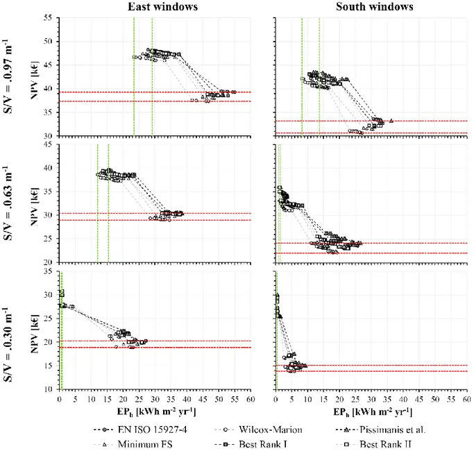
performance of the six reference years, while M5 is the closest one (+0.7 %). These findings are coherent with those in (Pernigotto et al., 2014b) for Trento, where Wilcox-Marion reference year gave the worst performance compared to the multi-year average heating needs while Best rank I gave the best one. The Pareto fronts are represented in Figure 2. The graphs show the trade-off between NPV and EPh
obtained for the six reference years. Two groups of results belonging to the fronts can be distinguished: the optimal solutions with mechanical ventilation system in the higher-left side of the chart (i.e., with higher NPV and lower EPh) and those with natural
ventilation in the lower-right side (i.e., with lower
NPV and higher EPh). The variability of weather
inputs is reflected in a shift of Pareto fronts. The front calculated with M2 is characterized by the lowest NPV and EPh while the one estimated with
M3 has often the highest NPV and EPh of the group
of six reference years. Indeed, Wilcox-Marion reference year leads to the prediction of a better energy performance of the initial configurations while reference year M3, developed according to Pissimanis et al., a worse performance is indicated for most of configurations.
In some cases, there are also intersections of Pareto curves calculated from the different reference years, even if this behaviour seems less marked than the one observed in previous works in case of reference years developed with EN ISO 15927-4 method from historic series of different length (Prada et al., 2014).
Table 3
Annual primary energy for space heating and net present values for the initial existing buildings according to the six different reference years
EPh [kWh m-2 yr-1] S/V Orientation M1 M2 M3 M4 M5 M6 Avg. Std. dev. 0.30 East 154.2 143.2 154.6 149.6 153.3 153.3 151.4 2.9 % South 119.7 106.5 122.1 112.6 116.7 116.9 115.8 4.8 % 0.63 East 231.9 217.6 230.8 225.3 229.2 230.1 227.5 2.3 % South 197.9 181.9 200.4 190.3 194.6 195.5 193.4 3.4 % East 294.7 280.9 292.7 288.7 291.9 292.9 290.3 1.7 % South 264.9 248.2 266.8 256.7 260.8 261.9 259.9 2.6 % NPV [€] S/V Orientation M1 M2 M3 M4 M5 M6 Avg. Std. dev. 0.30 East 42 666 39 658 42 764 41 406 42 415 42 426 41 889 2.9 % South 33 283 29 672 33 910 31 347 32 456 32 502 32 195 4.7 % 0.63 East 63 828 59 926 63 522 62 017 63 107 63 315 62 619 2.3 % South 54 553 50 227 55 233 52 485 53 671 53 896 53 344 3.3 % East 80 910 77 180 80 360 79 292 80 178 80 448 79 728 1.7 % South 72 817 68 257 73 310 70 564 71 680 72 008 71 439 2.6 %
Figure 2 - Pareto fronts for the different building configurations. The green vertical lines delimitate the spread between the energy optima while the red horizontal lines the spread between the cost optima found with the six
different reference years
For instance, in the case of S/V = 0.63 m-1 with South-faced windows, considering the group of configurations with natural ventilation, the Pareto front with highest NVP and EPh is with the reference
year M3, whereas for the group of configurations with mechanical ventilation the Pareto front with highest NVP and EPh is with the reference year M5.
Cost optimal
In order to evaluate in detail the effects of the different reference years on the cost-optimal solution, the ESM configurations of Pareto front ensuring the minimum of a single objective have been analysed, starting from the NPV.
As it can be seen in Tables 4 and 5, the ESMs optimizing the economic objective are the adoption of double glazing and natural ventilation. The only exception is the semi-detached house with East-oriented windows, for which the reference year M3
leads to the recommendation of replacing the original windows with triple glazing. For cases with S/V = 0.3 m-1 and both East and South-faced windows and those with S/V = 0.63 m-1 and South-oriented windows, no substitution of the boiler is suggested. For the remaining configurations, the modulating boiler is preferred for buildings with South-faced windows and the condensing boiler for buildings with East-faced windows. For the latter, the reference year affects the choice of the new boiler: for instance, the penthouse can be optimized with a modulating boiler if simulated with reference year M2, while, if the other reference years are used, the optimum can be achieved with a condensing boiler. As regards the optimal insulation, a greater variability is found, especially for the configurations with South-oriented windows. As a whole, the uncertainty in the NPV of the cost-optimal solutions ranges between 1000 and
3000 €, increasing when building configurations with larger S/V and energy demands are considered. Energy optimal
The energy optimal configurations present slight differences in terms of ESMs especially in East-oriented cases, but have different EPh because of the
different weather file used (Tables 4 and 5). The insulation thickness is generally equal or close to the maximum allowable (i.e., 20 cm) with the exception of the building with S/V = 0.3 m-1 and South-oriented windows, whose optimal insulation ranges from 13 cm (reference years M1, M4 and M6) to 18 cm (reference year M3). The original windows are almost always changed with triple-pane glazing
systems: they have always high SHGC, excluding the intermediate flats with windows on the South façade, for which triple glazing with low SHGC are preferred for all reference years except M1, and the semi-detached house with South-oriented windows, for which double glazing with high SHGC is the best solution with reference year M6.
Mechanical ventilation system is always adopted, independently of the reference year. As regards the boiler, the condensing one is the prevalent optimal solution but for the building with S/V = 0.3 m-1 and East-oriented windows, if reference year is M2 or M3, no replacement is suggested.
Table 4
EPh [kWh m-2 yr-1] and NPV [k€] for the building configurations with East-oriented windows according to the
six reference years: characteristics of energy and cost-optima
Table 5
EPh [kWh m-2 yr-1] and NPV [k€] for the building configurations with South-oriented windows according to the
six reference years: characteristics of energy and cost-optima
M1 M2 M3 M4 M5 M6 M1 M2 M3 M4 M5 M6 M1 M2 M3 M4 M5 M6 Energy-Optimal Wall 20 20 20 20 20 20 20 19 19 19 19 20 20 19 18 19 18 18 Roof 0 0 0 0 0 0 19 19 19 20 20 20 20 19 19 19 19 19 Floor 0 0 0 0 0 0 0 0 0 0 0 0 20 20 20 20 19 19 Wind. TH TH TH TH TH TH TH TH TH TH TH TH TH TH TH TH TH TH
Boiler COND STD STD COND COND COND COND COND COND COND COND COND COND COND COND COND COND COND Vent. M VS M VS M VS M VS M VS M VS M VS M VS M VS M VS M VS M VS M VS M VS M VS M VS M VS M VS EPH 0.55 0.73 0.62 0.93 0.93 0.89 15.39 12.08 15.35 12.87 14.01 13.68 27.84 23.43 28.69 26.17 29.20 29.13 NPV 30.74 27.91 27.88 30.84 30.84 30.83 39.61 38.57 39.47 39.00 39.31 39.35 48.24 46.70 48.00 47.45 47.93 47.91 Cost-Optimal Wall 19 17 18 19 19 18 18 18 17 17 17 17 19 18 17 18 16 18 Roof 0 0 0 0 0 0 17 19 17 17 17 17 19 17 18 18 17 18 Floor 0 0 0 0 0 0 0 0 0 0 0 0 18 18 18 18 17 19 Wind. DH DH TH DH DH DH DH DH DH DH DH DH DH DH DH DH DH DH
Boiler STD STD STD STD STD STD COND M OD COND COND COND COND M OD COND COND COND COND COND Vent. NAT NAT NAT NAT NAT NAT NAT NAT NAT NAT NAT NAT NAT NAT NAT NAT NAT NAT EPH 27.23 23.23 23.27 24.62 25.84 26.48 38.27 34.59 38.60 36.24 38.03 37.91 55.09 46.87 51.46 48.56 52.93 49.80 NPV 20.23 18.88 20.18 19.52 19.85 19.89 30.40 28.92 30.35 29.71 30.20 30.16 39.26 37.36 38.68 38.03 38.54 38.57 East S /V = 0.3 m -1 S /V = 0.63 m-1 S /V = 0.97 m-1 M1 M2 M3 M4 M5 M6 M1 M2 M3 M4 M5 M6 M1 M2 M3 M4 M5 M6 Energy-Optimal Wall 13 16 18 13 14 13 20 20 20 20 20 20 19 19 19 18 18 18 Roof 0 0 0 0 0 0 20 20 20 20 20 20 19 19 19 17 19 19 Floor 0 0 0 0 0 0 0 0 0 0 0 0 18 18 20 18 20 16 Wind. TH TL TL TL TL TL TH TH TH TH TH TH TH TH TH TH TH DH
Boiler COND COND COND COND COND COND COND COND COND COND COND COND COND COND COND COND COND COND Vent. M VS M VS M VS M VS M VS M VS M VS M VS M VS M VS M VS M VS M VS M VS M VS M VS M VS M VS EPH 0.54 0.52 0.54 0.53 0.52 0.51 1.42 1.01 1.54 1.36 1.33 1.30 11.23 8.21 11.88 10.93 10.56 13.69 NPV 29.81 29.83 30.10 29.43 29.57 29.43 36.01 35.90 36.04 36.00 35.99 35.98 42.97 42.14 43.56 42.34 43.06 41.93 Cost-Optimal Wall 17 15 17 14 18 18 17 16 18 17 17 17 17 18 17 17 17 17 Roof 0 0 0 0 0 0 15 17 16 18 16 16 18 16 18 17 17 17 Floor 0 0 0 0 0 0 0 0 0 0 0 0 17 17 16 16 18 16 Wind. DH DH DH DH DH DH DH DH DH DH DH DH DH DH DH DH DH DH Boiler STD STD STD STD STD STD STD STD STD STD STD STD M OD M OD M OD M OD M OD M OD Vent. NAT NAT NAT NAT NAT NAT NAT NAT NAT NAT NAT NAT NAT NAT NAT NAT NAT NAT EPH 8.02 5.92 9.39 7.76 6.83 6.81 25.78 19.21 26.71 19.13 22.97 22.95 33.61 27.15 36.25 30.48 30.99 32.96
NPV 14.73 13.90 15.11 14.26 14.54 14.54 23.57 22.06 24.17 22.38 23.01 23.01 32.73 30.69 33.24 31.46 32.02 32.14
S outh S /V = 0.3 m
-1
Considering the uncertainty in the EPh of the
energy-optimal solutions, it is almost null for the most compact buildings and about 5 kWh m-2 yr-1 for those with the highest S/V.
CONCLUSION
In this work, the robustness of a genetic algorithm, the Elitist Non-dominated Sorting Genetic Algorithm, was assessed in the framework of multi-objective optimizations of building energy refurbishment through building energy simulation. In particular, the focus was on the issues due to suboptimal hourly weather data and on the impact of the method for the development of reference years. Six reference years implementing just as many different methods were developed for the location of Trento, north Italy. These reference years were used as inputs for the refurbishment multi-objective optimization of six buildings with three ratios between the externally exposed surface and the conditioned volume and two alternatives of windows orientations. Among the available energy saving measures for the reduction of final uses for space heating, wall insulation, windows and boiler substitutions and installation of a mechanical ventilation system with heat recovery were considered. The optimization involved the trade-off between primary energy for space heating and net present value of the investment, which were studied in terms of Pareto fronts.
Since each reference year gave specific initial conditions of EPh and NPV, different Pareto fronts
were found for each building configuration. However, the results showed that fronts are not simply shifted on the NPV-EPh chart but, in some
cases, they can have different shapes and propose different optimal solutions.
The actual choice of the optimal ESM in Pareto front depends on the weights given to the objectives in trade-off. In order to analyse which ESMs are more sensitive to the weather data input, two separate studies were performed to look for (a) the ESM optimizing the NPV and (b) the one optimizing the
EPh among those on Pareto fronts. According to the
building kind, different sensitivities were found but, in general, the insulation level and the boiler replacement presented the largest variability, which was more emphasized in the NPV optimization context. The selection of the best solution for window substitution demonstrated to be, to some extent, more robust to the weather inputs. As regards the ventilation, no sensitivity at all was detected for the considered buildings.
The results of this study confirmed the findings found in previous works (Prada et al., 2014) about weather inputs, allowing us to conclude that if some representativeness issues are present in the reference years – because of either the methodology for the reference year definition or the inadequacy of the historic multi-year weather data series, different
optimal ESMs can be identified through the multi-objective optimization.
NOMENCLATURE
A = surface (m2)
BES = building energy simulation c = specific heat (J kg-1 K-1)
d = thickness (m) COND = condensing boiler D = double glazings
EP = primary energy (kWh m-2 yr-1)
ESM = energy saving measure FS = Finkelstein–Schafer statistic H = high SHGC
HDD = heating degree days (K d) GA = genetic algorithm
I = solar irradiation (MJ m-2 d-1)
= thermal conductivity (W m-1 K-1)
L = low SHGC
κ = thermal capacitance (kJ m-2 K-1)
MOD = modulating boiler MVS = mechanical ventilation NAT = natural ventilation NPV = net present value (€)
R = thermal resistance (m2 K W-1)
= specific mass (kg m-3)
S = envelope exposed surface (m2)
SHGC = solar heat gain coefficient (-) STD = standard boiler T = triple glazings U = thermal transmittance (W m-2K-1) V = conditioned volume (m3) Subscript fr = frame gl = glazing h = heating sol = solar win = window
REFERENCES
ASHRAE. 2006. ANSI/ASHRAE Standard 169, Weather data for building design standards. Atlanta, U.S.
Brownlee, A.E., Wright, J.A., Mourshed, M.M. 2011. A multi-objective window optimisation problem. Proc. of the 13th annual conference companion on genetic and evolutionary computation. Burjorjee, K.M. 2013. Explaining optimization in
genetic algorithms with uniform crossover. Proc. of Foundations of Genetic Algorithms, 37-50. Burhenne, S., Jacob, D., Henze, G.P. 2011. Sampling
based on Sobol’s sequences for Monte Carlo techniques applied to building simulations. Proc. of 12th Building Simulation, 1816-1823.
Deb, K. 2002. A fast and elitist multi-objective genetic algorithm: NSGA-II. IEEE transactions on evolutionary computation, 6(2):182-197. European Commission 2010. Directive 2010/31/EU
Official Journal of European Union, L 153/13, 18/06/2010, Brussels, Belgium.
European Commission 2012. Commission Delegated Regulation (EU) No 244/2012 of 16 January 2012 supplementing Directive 2010/31/EU. Official Journal of European Union, L 81/18, 21/03/2012, Brussels, Belgium.
European Committee for Standardization (CEN) 1999. EN 12207:1999 - Windows and doors. Air permeability – Classification, Brussels, Belgium. European Committee for Standardization (CEN) 2005. EN ISO 15927-4:2005 - Hygrothermal performance of buildings - Calculation and presentation of climatic data - Part 4: Hourly data for assessing the annual energy use for heating and cooling, Brussels, Belgium.
European Committee for Standardization (CEN) 2007a. EN ISO 10211:2007 - Thermal bridges in building construction - Heat flows and surface temperatures - Detailed calculations, Brussels, Belgium.
European Committee for Standardization (CEN) 2007b. EN 15242:2007 - Ventilation for buildings – Calculation method for the determination of air flow rates in buildings including infiltration, Brussels, Belgium. European Committee for Standardization (CEN)
2007c. EN 15251:2007 - Indoor environmental input parameters for design and assessment of energy performance of buildings addressing indoor air quality, thermal environment, lighting and acoustics, Brussels, Belgium.
European Committee for Standardization (CEN) 2009. EN 15459:2009 - Energy performance of buildings - Economic evaluation procedure for energy systems in buildings, Brussels, Belgium. Evins, R. 2013. A review of computational
optimisation methods applied to sustainable building design. Renewable and Sustainable Energy Reviews, 22:230–245.
Goldberg, D.E., Korb, B., Deb, K. 1989. Messy genetic algorithms: motivation, analysis, and first results. Complex Systems, 3(5):493-530. Goldberg, D.E., Deb, K. 1991. A comparative
analysis of selection schemes used in genetic algorithms. Proc. of Foundations of Genetic Algorithms, 69-93.
Haller, M.Y., Paavilainen, J., Konersmann, L., Haberl, R., Dröscher, A., Frank, E., Bales, C., Streicher, W. 2011a. A unified model for the simulation of oil, gas and biomass space heating boilers for energy estimating purposes. Part I: Model development. Journal of Building Performance Simulation, 4(1):1–18.
Haller, M.Y., Paavilainen, J., Konersmann, L., Haberl, R., Dröscher, A., Frank, E., Bales, C., Streicher, W. 2011b. A unified model for the simulation of oil, gas and biomass space heating boilers for energy estimating purposes. Part II: Parameterization and comparison with
measurements. Journal of Building Performance Simulation, 4(1):19–36.
Hopfe, C.J., Hensen, J.L.M. 2011. Uncertainty analysis in building performance simulation for design support. Energy and Buildings, 43: 2798– 2805.
Ihm P., Krarti M. 2012. Design optimization of energy efficient residential buildings in Tunisia. Building and Environment, 58:81-90.
Jena, S., Patro, P., Behera, S.S. 2013. Multi-Objective optimization of design parameters of a shell and tube type heat exchanger using Genetic Algorithm. International Journal of Current Engineering and Technology, 3(4): 1379-1386. Matsumoto, M., Nishimura, T. 1998. Mersenne
Twister: a 623-dimensionally equidistributed uniform pseudo-random number generator. ACM Transactions on Modeling and Computer Simulation, 8(1):3-30.
Penna, P., Prada, A., Cappelletti, F., Gasparella, A. 2015. Multi-objectives optimization of energy efficiency measures in existing buildings. Energy and Buildings, 95:57–69.
Perez, R., Stewart, R., Seals, R., Guertin, T. 1988. The development and verification of the Perez diffuse radiation model. Sandia Report SAND88-7030, Albany, U.S.
Pernigotto, G., Prada, A., Cóstola, D., Gasparella, A., Hensen, J.L.M. 2014a. Multi-year and reference year weather data for building energy labelling in north Italy climates. Energy and Buildings, 72:62-72.
Pernigotto, G., Prada, A., Gasparella, A., Hensen, J.L.M. 2014b. Analysis and Improvement of the representativeness of EN ISO 15927-4 reference years for building energy simulation. Journal of Building Performance Simulation, 7(6):391-410. Pissimanis, D.K., Karras, G.S., Notaridou, V.A.,
Gavra, K. 1988. The Generation of a ‘Typical Meteorological Year’ for the City of Athens. Solar Energy, 40(5):405–411.
Prada, A., Pernigotto, G., Cappelletti, F., Gasparella, A., Hensen, J.L.M. 2014. Robustness of multi-objective optimization of building refurbishment to suboptimal weather data. III International High Performance Buildings Conference at Purdue, West Lafayette, Indiana, U.S.
Reindl, D., Beckman, A., Duffie, J.A. 1990. Diffuse fraction correlations. Solar Energy, 45(1):1–7. Saltelli, A., Tarantola, S., Campolongo, F., Ratto, M.
2004. Sample generation, in Sensitivity analysis in practice. A guide to assessing scientific models, Chichester (UK): John Wiley & Sons, 193-204.
Wilcox, S.M., Marion, W. 2008. Users Manual for TMY3 Data Sets. Golden, Colorado, U.S. Wright, J., Alajmi, A. 2005. The robustness of
genetic algorithms in solving unconstrained building optimization problems. Proc. of 9th