Embedded Real Time Gesture
Tracking
Candidato:
Relatori:
Giuseppe Arturi
Prof. Luca Fanucci
Prof. Luciano Lenzini
Dr. Ir. Richard Kleihorst
dato l’opportunit`a di intraprendere quest’avventura.
Infine (the last but not the least) voglio sentitamente ringraziare Angelo, Claudio, Giovanni e Davide che hanno reso questa esperienza decisamente interessante.
Guiseppe Pisa - 28 Febbraio 2008
2.1 WiCa architecture . . . 9
2.2 Hardware components . . . 10
2.2.1 Xetal IC3D . . . 10
2.2.2 Host controller 8051 . . . 11
2.2.3 SRAM . . . 12
2.2.4 Aquis grain ZigBee module . . . 12
2.3 Programming Xetal . . . 13
3 Video Tracking: Overview 14 3.1 In-Node Features Extraction . . . 15
3.1.1 Edge Detection . . . 17 3.1.2 Background Subtraction . . . 18 3.1.3 Image Segmentation . . . 19 3.1.4 Tracking . . . 20 4 Tracking on WiCa 21 4.1 Algorithms on WiCa . . . 21 4.1.1 Edge Detection . . . 21 4.1.2 Background Subtraction . . . 22 4.1.3 Image Segmentation . . . 30 4.1.4 Tracking . . . 32 1
Bibliography 54 A Background Subtraction Proofs and Examples 56 A.1 Proof of 4.8 . . . 56 A.2 Example of Block-based Background Subtraction . . . 57
B XTC Code 62
B.1 K-means . . . 62 B.2 Tracking . . . 63 C Single Thresholding Process 66
2.6 Architecture of the IC3D which is a member of the Xetal
fam-ily of SIMD chips. . . 10
2.7 AquisGrain v2.0 ZigBee. . . 12
3.1 Camera Network scheme. . . 15
3.2 In-node features extraction scheme : Serial Approach. . . 16
3.3 In-node features extraction scheme : Parallel Approach. . . 16
3.4 Tracking process in a single camera using motion detection. . . 17
3.5 Tracking process in a single camera using edge detection. . . . 18
4.1 Sobel filter : horizontal direction. . . 23
4.2 Sobel filter : vertical direction. . . 23
4.3 . . . 26
4.4 Background Subtraction Block-Based screenshot one. . . 28
4.5 Background Subtraction Block-Based screenshot two. . . 28
4.6 Background Subtraction Pixel-Based Scheme. . . 29
4.7 Background Subtraction Pixel-Based screenshot one. . . 29
4.8 Background Subtraction Pixel-Based screenshot two. . . 29
4.9 Skin tone segmentation. . . 31
4.10 Skin tone segmentation and Background Subtraction. . . 31
4.11 Experimental results of tracking without recovery. . . 34
4.12 Experimental results of tracking without recovery with object lost. Frames 6, 7 and 8 show a failing of tracking probably because of acceleration. . . 35
5.11 Motion density detection and skintone segmentation. . . 46
5.12 Edge density detection and skintone segmentation. . . 47
5.13 Experimental results of gesture tracking : first sequence. . . . 49
5.14 Experimental results of gesture tracking : second sequence. . . 50
5.15 Experimental results of gesture tracking : third sequence. . . . 51
A.1 . . . 58
A.2 . . . 59
A.3 . . . 60
A.4 . . . 60
A.5 . . . 61
C.1 In-node features extraction parallel scheme : skin-like moving object. . . 66
Ambient intelligence is defined as electronic environments that are aware of and responsive to the presence of people. Ambient intelligence is a lively field of research, pushing technology and relevant applications. So far, most applications are focused toward monitoring scenes and persons.
Imaging could play and plays an important role in sensing devices for ambient intelligence [1, 2]. Computer vision can for instance be used for recognizing persons and objects and recognizing behavior such as illness and rioting.
Tracking hands and head is important because human being movements interpretation could potentially be used to interact with electronic systems in more natural ways. For example, head and hands gestures and motions are needed for gaming or for interact with computers.
In order to build handy applications time constraints are needful, so that a real time system is required. Furthermore, a non-invasive technology is highly necessary in specific environments.
The main body of this paper is divided as follows. Chapter 2 describes the hardware used during this work. The Wireless camera (WiCa) developed by NXP Semiconductor combines an SIMD processor (Xetal/IC3D) for low-level operations, an 8051 microprocessor for high-low-level operations, RAM for inter-frame processing and a ZigBee transmitter for communication [1, 2]. A non-volatile memory is used to store programs for the IC3D.
Chapter 3 is a brief panoramic on image segmentation, edge detection, background subtraction, tracking and how to combine these technique to obtain the final result.
(WiCa)
Real-time video processing on (low-cost and low-power) programmable is now becoming possible thanks to advances in integration techniques [1, 4]. It is important that these platform are programmable since new vision methods and applications emerge every month.
The algorithms in the application areas of smart cameras can be grouped into three levels: low-level, intermediate level and high-level tasks. Figure 2.2 and Figure 2.3 show the task level classification and the corresponding data entries respectively.
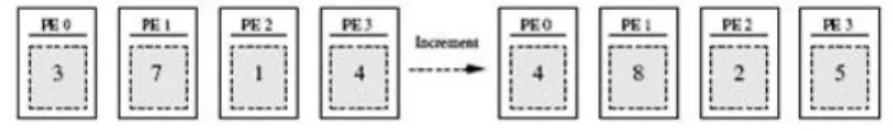
The low- or early-image processing level is associated with typical kernel operations like convolution and data-dependent operations using a limited neighborhood of the current pixel. In this part, often a classification or the initial steps toward pixel classification are performed. Because every pixel could be classified in the end as ’interesting’, the algorithms per pixel are essentially the same. So, if more performance is needed in this level of image processing, with up to a billion pixels per second, it is very fruitful to use this inherent data parallelism by operating on more pixels per clock cycle. The processors exploiting this have an SIMD 1 architecture, where the same
instruction is issued on all data pixels in parallel [5].
1Single Instruction Multiple Data
Figure 2.1: SIMD example.
From a power consumption point of view, SIMD processors prove to be economical. The parallel architecture reduces the number of memory ac-cesses, clock speed, and instruction decoding, thereby enabling higher arith-metic performance at lower power consumption [1, 4].
In the high- and intermediate-level part of image processing, decisions are made and forwarded to the user. General purpose processors are ideal for these tasks because they offer the flexibility to implement complex soft-ware jobs and are often capable of running an operating system and doing networking applications.
Figure 2.2: Algorithm classifica-tion with respect to the type of op-erations.
Figure 2.3: Data entities with pro-cessing characteristics and possible ways to increase performance by exploiting parallelism.
with a power consumption of less than 200mW. A top level schematic of the architecture is depicted in figure 2.5.
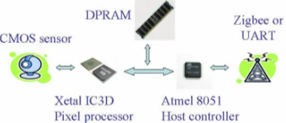
The smart camera used is the second one of the WiCa family (WiCa 1.1). The basic components are : one or two VGA color image sensors, a SIMD processor for low-level image processing (IC3D), a general purpose processor for intermediate and high-level processing and control (8051 microprocessor), a communication module (ZigBee transmitter) and a static RAM (SRAM) (Figure 2.4. The presence of an SRAM, instead of dual port RAM (the previous WiCa had a DPRAM), needs some kind of arbitration to allow Xetal and 8051 access memory like pseudo-dual port. This feature is employed inside a CPLD Cool Runner 2 component and it is transparent to WiCa users.
Figure 2.4: WiCa top architecture. A brief explanation of the principal components is given.
2.2
Hardware components
2.2.1
Xetal IC3D
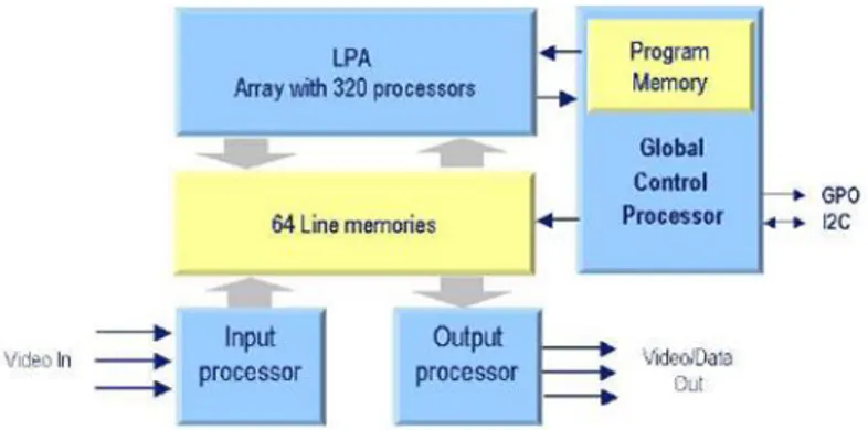
The IC3D, a member of the NXP’s Xetal family of SIMD processor, is com-posed by five specific internal blocks, see figure 2.6. Two blocks function as
Figure 2.5: WiCa 1.1 hardware components.
video input and video output processors respectively. They are capable of generating three digital video signals towards the internal memory.
Figure 2.6: Architecture of the IC3D which is a member of the Xetal family of SIMD chips.
The heart of the chip is formed by the Linear Processor Array (LPA) with 320 RISC processors. Each of these processors can access (read and write) within one clock cycle to memory positions in the parallel memory. Both the memory address and the instruction of the processors are shared in SIMD sense. All processors can also read the memory data of their left and right neighbors directly. Data paths are 10-bits wide and each processor has two word registers and one flag register.
The line-memory block stores 64 lines of 3200 bits. Pixels of the im-age lines are placed in an interlaced way on this memory. So, CIF imim-ages (320x240) result in one pixel per processor, VGA images (640x480) in two pixels per processor, etc.
The IC3D can communicate with 8051 via I2C, via SRAM and via inter-rupt3.
2.2.2
Host controller 8051
As host controller an ATMEL 8051 is used. This device has all necessary components inside to make a small, yet complete, system. It is geared of a large number of usable I/O pins to control the camera and its surroundings. The 8051 has a 16 bit-wide external address bus for memory which fits easily to the memory connected to the IC3D.
To indicate special data transfers between the IC3D and 8051, an inter-rupt line on the 8051 is used that can be triggered by IC3D. The used 8051 has 1792 bytes of internal RAM and 64kbyte of Flash to store its program or additional data. The internal 2KB EEPROM is used to store parameters and instruction code for the IC3D. Communication to the outside world is done via the UART. The UART has its own baud rate generator so all three timers of the 8051 are available for user applications. There are two 8 bit timers and one 16bit timer. They are now partly used for task-switching in a (tiny) operating system.
2.2.3
SRAM
The CMOS Static RAM is organized as 512K x 8 bits. This memory replaces the 128 KB DPRAM used in WiCa 1.0. The main difference is that the new capacity is 4 times larger. That means that WiCa 1.1 has 8 different blocks available of 64KB that could be accessed by Xetal or 8051, so that it is possibile to store up to 4 VGA images in the main memory. The second
2Giga Operations Per Second
Figure 2.7.
Figure 2.7: AquisGrain v2.0 ZigBee.
The radio system implementation and general properties are very similar to v1.0. The most important difference is, obviously, the size of the new device. The antenna is integrated in the same board, as well as the new CC2430 integrates the old CC2420 RF system plus an 8051 controller. A real SoC that enables reduce au maximum the final area of this device.
The communication module is still attached to the camera as a wireless UART port. But now, the maximum data-rate has increased up 250kb/Sec-ond thanks to the new USB device integrated in the WiCa 1.1.
2.3
Programming Xetal
The Xetal chip is programmed using and extended C (XTC) language, a sample code shown belowe.
do {
W a i t l i n e ( ) ; // Hsynch
yuv=s e n s o r 1 y u v ( ) ; // A c q u i r e s from s e n s o r
yuv [ 0 ] [ 0 ] = 0 . 5 ∗ yuv [ 0 ] [ 0 ] . n e i g h ( −1) + 0 . 5 ∗ yuv [ 0 ] [ 0 ] . n e i g h ( 1 ) ; rgb=YUVtoRGB( yuv ) ; // C o l o r s p a c e model c o n v e r s i o n
WriteToLCD ( rgb ) ; // O u t p u t s on LCD u s e d f o r d e b u g g i n g p u r p o s e s f i n a l i z e O u t p u t ( ) ;
} while(++c u r r e n t r o w < 4 8 3 ) ; }
One of the major extensions is the introduction of the vector data type (vint or lmem) to represent the 320-element wide read-write memory in the LPA. The remaining data are represented in a 16-bit integer or fixed point. In the example code, the functions neigh(-1) and neigh(1) are used to access left and right neighbors, respectively. The optional neigh(0) represents the data directly connected to each PP.
the location of moving targets within the video frame. The main difficulty in video tracking is to associate target locations in consecutive video frames, especially when the objects are moving fast or accelerating relative to the frame rate.
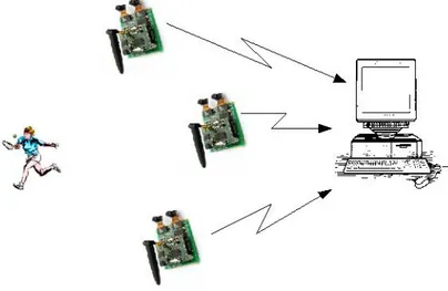
Tracking in a single camera suffers from occlusion and makes the estima-tion of the object movements difficult;when a single camera is not sufficient to detect and track objects due to limited visibility or occlusion, multiple cameras can be employed. A multi camera system (or camera network) consists of a set of cameras, communication infrastructure and computation units. Typically each camera is connected to a PC which receives the infor-mation extracted in the cameras and, based on this inforinfor-mations, infers more complex knowledge. A scheme is shown in Figure 3.1.
One underlying constraint of the network is the relatively low bandwidth. Therefore, for efficient collaboration between cameras, we need concise de-scriptions instead of raw image data as outputs from local processing in a single camera. So that, each camera performs its local processing to extract the features needed to estimate the behavior of moving objects.
For most tasks, a multi camera system has to be calibrated. Depending on the application, the type of calibration information which is required can be very different. Possible calibrations vary from a simple neighborhood structure identifying cameras with a common field of view to a full metric calibration, which consists of the internal parameters of each camera as well
Figure 3.1: Camera Network scheme.
as the (relative) positions and orientations of the cameras [13, 12].
3.1
In-Node Features Extraction
The aim of this process is a concise representation of the raw image data input. This process inevitably removes certain details in images of a sin-gle camera, which requires the camera to have some “intelligence“ on its observations (smart cameras), i.e., some knowledge of the subject.
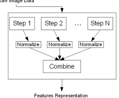
The process that allows to achieve the goal can be described as shown in Figure 3.2
At each step, the data is refined in order to achieve the goal. One or more steps can be exploited in the same level in order to produce the input data for the following step. The output of the process, is a concise representation of the feature desired.
Another approach, shown in Figure 3.3, can be used. The main different is that the features are normalized and combined together before inferring knowledges about the object of interest.
The algorithm executed in each steps depends on the application. If the goal is to localize a moving object, a possible implementation can be seen in figure 3.4.
As can be seen, this procedure requires three steps: background subtrac-tion, image segmentation and tracking.
Figure 3.2: In-node features extraction scheme : Serial Approach.
Figure 3.4: Tracking process in a single camera using motion detection. The Background Subtraction block provides a method to isolate the ob-jects of interest from the background, thus the output is a rough estimation of the tracked objects. This information is given in input to the second block (Segmentation) that refine the previous data in order to select the moving objects basing on their characteristics (for example an image segmentation based on a color can select the skin tone to follow the hands and the face). The Tracking block can compute the positions of the objects thanks to the output data given by the previous block and information from the previous frame.
Instead of using movements detection is it possible to employ edge detec-tion as is shown in Figure 3.5.
3.1.1
Edge Detection
The aim of this process is to select the pixels in a digital image basing on the sharply changes in the luminance intensity. Edge detection is useful in order to select relevant information in an image while preserving the important structural properties.
Figure 3.5: Tracking process in a single camera using edge detection. Search based detects edge by looking for maximum and minimum in the
first derivative of the image (usually local directional maximum of the gradient magnitude).
Zero-crossed based searches for zero crossing in the second derivative of the image.
In Chapter 4 the Sobel filter is described.
3.1.2
Background Subtraction
A common approach in order to identifying moving objects from a video se-quence is to perform background subtraction.The aim is to identify moving objects from the portion of a video frame that differs significantly from a background model. This process must be robust against changes in illumi-nation, it should avoid detecting non-stationary background objects such as moving leaves, rain, and shadows cast by moving objects and its internal background model should react quickly to changes in background. These challenges has to be taken into account so that the algorithm works well.
tracked homogeneous regions and then apply further processing to identify the objects. Many different video segmentation techniques exist [7]. For example, it is possible to carry image segmentation algorithms, such as color or texture segmentation, to generate homogeneous regions in each frame and then track the motion of the segmented regions.
Several general-purpose algorithms and techniques have been developed for image segmentation. Since there is no general solution to the image seg-mentation problem, these techniques often have to be combined with domain knowledge in order to effectively solve an image segmentation problem for a problem domain.
Clustering Clustering is a feature-space based technique in which classes are generated (or partitioned) without any a priori knowledge. The K-means algorithm belongs to this class of methods; it is an iterative technique that is used to partition an image into K clusters [8];
Histogram thresholding Histogram-based methods are very efficient when compared to other image segmentation methods because they typically require only one pass through the pixels. In this technique, a histogram is computed from all of the pixels in the image, and the peaks and val-leys in the histogram are used to locate the clusters in the image. Color or intensity can be used as the measure;
Region growing In the region growing techniques, a region is started with a single pixel. Adjacent pixels are recursively checked and added to the region if they are sufficiently similar to the region. If a pixel is too dissimilar to the current region, it is used to start a new region. At every step a pixel, not yet allocated, and close to at least a region, is allocated to an adjacent region that is more similar basing on the chosen criterion;
Edge Detection Edge detection is a well-developed field on its own within image processing. Region boundaries and edges are closely related, since there is often a sharp adjustment in intensity at the region bound-aries. Edge detection techniques have therefore been used to as the base
3.1.4
Tracking
The final step of the tracking process is to localize the objects of interest in every frame during time. There are two major components of a visual tracking system; Target Representation and Localization and Filtering and Data Association.
Some common Target Representation and Localization are listed below; this kind of algorithms are mostly based on a bottom-up process. Typically the computational complexity for these algorithms is low.
Blob tracking Segmentation of object interior (for example blob detection, block-based correlation or optical flow)[15];
Kernel-based tracking An iterative localization procedure based on the maximization of a similarity measure(Mean-shift)[9];
Contour tracking Detection of object boundary (e.g. active contours)[14]; Filtering and Data Association is mainly a top-down process, which in-volves incorporating prior information about the scene or object, dealing with object dynamics, and evaluation of different hypotheses. The computa-tional complexity for these algorithms is usually much higher. Some common algorithms are Kalman Filter [10] and Particle Filter [11].
In the chapter 4 a different method that uses the centers of mass of the segmented objects is used.
4.1
Algorithms on WiCa
4.1.1
Edge Detection
The Sobel operator is employed to detect edges on WiCa. It is a discrete differentiation operator, computing an approximation of the gradient of the image intensity function. At each pixel the Sobel operator gives either the corresponding gradient vector or the norm of this vector. The operator com-putes the gradient of the image intensity so that the result is the largest possible increase from light to dark and the measurement of change in that direction. Therefore, the result describes how abruptly (or smoothly) the image changes are in each pixel, therefore how likely that pixel represents an edge.
Mathematically, the operator computes the convolution between the orig-inal image and two kernels giving as result the approximations of the deriva-tives (one for horizontal changes and one for vertical changes). Let A be the source image, Gx and Gy, that are the two images representing
respec-tively the horizontal and vertical derivatives approximations, are computed as follows :
tude and direction : G = q Gx2+ Gy2 (4.3) θ = arctanGy Gx (4.4) The Sobel filter implementation on WiCa uses the previous two lines, the current line and the closest left and right neighbors to compute the horizontal and vertical values at every pixel.
e d g e h = a ∗ l 1 . n e i g h ( −1) + a ∗ l 1 . n e i g h ( 0 ) + a ∗ l 1 . n e i g h ( 1 ) − a ∗ l 3 . n e i g h ( −1) − a ∗ l 3 . n e i g h ( 0 ) − a ∗ l 3 . n e i g h ( 1 ) ; e d g e v = a ∗ l 1 . n e i g h ( −1) − a ∗ l 1 . n e i g h ( 1 )
+ a ∗ l 2 . n e i g h ( −1) − a ∗ l 2 . n e i g h ( 1 ) + a ∗ l 3 . n e i g h ( −1) − a ∗ l 3 . n e i g h ( 1 ) ;
The thresholding mechanism is applied to select the edges.
e d g e h = e d g e h > HOR THRESHOLD ? 1 : 0 ;
e d g e v = e d g e v > VER THRESHOLD ? 1 : 0 ;
In Chapter 5 a combination of vertical and horizontal edge detection is explained, so that a single threshold is used.
Experimental Results
The thresholding applied to the output Sobel operator is shown in Figure 4.1 and Figure 4.2.
4.1.2
Background Subtraction
Two techniques have been implemented on WiCa. The major difference between these two methods is that one works with blocks and the other works
Figure 4.1: Sobel filter : horizontal direction.
basing on the differences arising between the averages of the blocks in differ-ent frames.
The thresholding mechanism is used to accomplish this task. More in de-tail, two thresholds are used : slow threshold and fast threshold ; because of this, two averages are computed during the time : fastaverage and slowaver-age. The former is a quickly updated background used to detect the moving objects while the latter is a slowly updated background used to remove the smears. Both are compared with the previous blockaverage. The slowaver-aging is used to deal with the limited changes that happen when an object enters in a block. When the object leaves the block, the latter becomes back-ground (if the object remains in the block for few time) because slowaverage did not change during this period thereby removing the smearing effect.
The algorithm can be characterized by the following pseudo code :
f o r e a c h frame
1. < d e t e r m i n e which b l o c k s have t o be d i s p l a y e d >
2. < compute t h e new v a l u e s o f f a s t a v e r a g e and s l o w a v e r a g e > 3. < compute t h e v a l u e o f b l o c k a v e r a g e >
end
The first step involves the values of fastaverage, slowaverage and blockav-erage computed at the previous frame; to accomplish the task, two thresholds are used : fast threshold and slow threshold. The thresholding mechanism is used to determine whether the blocks have to be displayed or no in the current frame:
|f astaverage − blockaverage| > f ast threshold (4.5) |slowaverage − blockaverage| > slow threshold (4.6)
(concerning to the previous frame) that has to be used, while the latter de-cides how fast slowaverage is updated when the average of the block changes its value.
The third step calculates the average of every blocks in the current frame. Computation of fastaverage
Fast average is used to detect moving objects, its computation (for each component YUV) concerns two parameters : α and fast threshold. The test is accomplished carrying out the equation 4.5 while fastaverage is the convex combination of fastaverage and blockaverage as shown in 4.7
f astaverage = α ∗ f astaverage + (1 − α) ∗ blockaverage (4.7) It is possible to write 4.5 into formulas that allows us to better understand how the condition is affected by the changes in the blockaverage (a proof of 4.8 is given in Appendix A).
|
i
X
j=1
αi−j ∗ (yj−1− yj)| > λ (4.8)
where fastaverage and blockaverage have been replaced with x and y re-spectively, fast threshold with λ and i is the current frame.
The term inside the absolute operator is a weighted sum of the differences between blockaverages computed in adjacent frames. Thus, at frame i + 1, the previously computed blockaverages (weighted) are summed to check for the validity of 4.8.
As can be seen, since α is in the [0,1) interval, the last differences have higher weight than the first differences; how the weights are distributed is appointed by the value of α. Figure 4.3 shows the curves of αi−j (for i=100)
with different values of α.
The values close to the origin are the weights of the last blockaverages differences, that is, when α decrease it is considered just the last differences
Figure 4.3: .
while when α increase more previously computed differences are taken into account. This means that, with low values of α, it is troublesome to detect slow objects because the differences are small hence they are not high enough to overcome the threshold (this means that α should be controlled by the tracking informations). Because of this, only the boundaries are shown when the objects move on the screen. Setting α to its lowest possible value, i.e. 0, only the previous one difference is used, hence, the objects disappear from the screen immediately (motion difference).
On the other hand, with high values of α, the slow moving objects are easily detected, but they become background slowly, so they are visible even if they do not move anymore. Setting α to its highest possible value, i.e. 1, all the previous differences are used, so that, the objects never disappear from the screen (actually, the objects disappear,even if very slowly, thanks to the contribution of slowaverage).
Intermediate values of α introduces smear because objects are transferred to background with diminishings values.
In Appendix A an example is performed. Computation of slowaverage
Slowaverage is used to deal with the limited change that happen when an object enters in a block. When the object leaves the block, it disappears (if the object remains in the block for few frames) because slowaverage did not change (significantly) during this period.
The computation of slowaverage (for each components YUV) concerns two parameters : β and slow threshold. For every frame, slowaverage is
The first step is the same used in fastaverage computation, while the second steps is more complicated. More in detail, when blockaverage changes, slowaverage follows it very slowly. In fact, slowaverage is varied by 1 if and only if blockaverage differs (for more than 1) from slowaverage for at least β frames.
Thus, slowaverage is updated only if it differs steadily from fastaverage, that is, the object becomes background. The parameter β has to be large enough to avoid the smears. In fact, if slowaverage would change too quickly, the object would become background and when it leaves, the previous back-ground would be displayed as foreback-ground. It is clear that β and slow threshold are related. The former determines how fast the object become background, while the latter indicates when the object becomes background. It is impor-tant to clarify that slowaverage is needed to deal with the changes in the background, therefore, it has to be quite quick to absorb this transition, but it has not to be too fast to avoid that the moving object become background. Experimental Results
In Figure 4.4 and Figure 4.5 are shown the results of the algorithm imple-mented on WiCa.
Pixel-based technique
This technique is really simple but it needs a RAM memory to work; at every frame each pixel is compared with its luminance value in the previous frame so that, it is possible to apply the thresholding algorithm. Figure 4.6 shows the scheme of this approach. The rows acquired from the sensor are compared with the rows stored in the RAM to decide if the pixels are foreground or background. In order to compare the rows acquired from the sensor in the subsequent frame, the current row is sent also to the RAM.
Figure 4.4: Background Subtraction Block-Based screenshot one.
Figure 4.6: Background Subtraction Pixel-Based Scheme. Experimental Results
In Figure 4.7 and Figure 4.8 are shown the results of the algorithm imple-mented on WiCa.
Figure 4.7: Background
used to partition an image into K clusters. The basic algorithm is :
1. Choose K cluster centers, either randomly or based on same heuristic; 2. Assign each pixel to the closest cluster center;
3. Recompute the cluster centers using the current cluster memberships; 4. If a convergence criterion is not met, go to 2. (for example, minimal
reassignment of pixels to new cluster centers).
This algorithm is guaranteed to converge, but it may not return the opti-mal solution. The quality of the solution depends on the initial set of clusters and the value of K.
The algorithm implemented on WiCa is slightly different, the step 4 is not needed because of the real-time environment. During each frame, it is decided which pixel belongs to which class and the values of UV components are collected to update the centroids (cluster centers) at the end of the frame. In Appendix B the code that executes the k-means algorithm is per-formed.
Experimental Results
The result of the k-means algorithm implemented on WiCa that segments the skin tone is shown in Figure 4.9. As can be seen, the result is significant even if is still present noise due to skin-like color objects in the background. In order to remove the noise a combination of background subtraction and segmentation can be used. Therefore, the segmentation is applied and the background subtraction is carried out subsequently, the result is shown in Figure 4.10. As it possible to see, the noise disappears and the result is better for tracking purposes.
Figure 4.9: Skin tone segmentation.
pixels {~xi}i=1...k with ~xi ∈ N and given S(~x) be the square area, the center of mass is given by 4.9. ~c = P ~ xi∈S(~x)mi∗ ~xi P ~ xi∈S(~x)mi (4.9) In this case mi is computed as in 4.10.
mi =
(
1 if ~xi ∈ C(~x),
0 if ~xi ∈ C(~/ x).
(4.10) where C(~x) is the set of pixels that belong to the object tracked (as indicated by the segmentation).
In Appendix B the xtc code to track is shown. Object Recovery
The algorithm showed uses a simple motion model with constant velocity, so that if the object moves too fast it is lost. A strategy to recover from lost objects is employed. Every frame, the maximum concentration of pixels is searched in the neighborhood of the search area. When the object is lost, this zone is explored.
In the next section the experimental results, with and without the recov-ery strategy, are shown.
Experimental Results
The Figure 4.11 shows the outcome of the algorithm without object recovery, while in Figure 4.12 is shown a fail in tracking.
In Figure 4.13 are shown two different recovery from lost. Because of the different frame rate between the LCD screen and the webCam used to
(1) (2)
(3) (4)
(5) (6)
(7) (8)
(1) (2)
(3) (4)
(5) (6)
(7) (8)
Figure 4.12: Experimental results of tracking without recovery with object lost. Frames 6, 7 and 8 show a failing of tracking probably because of accel-eration.
(1) (2)
(3) (4)
(5) (6)
(7) (8)
Figure 4.13: Experimental results of tracking with recovery : two sequences, from (1) to (4) and from (5) to (8)
In order to get informations about human behavior it is needed to track in real time the movements. The goal of this work is to track human movements using the WiCa platform. Our assumption states that the orientation of the WiCa is such that the face is in front of the camera.
As shown in Chapter 4, it is possible to extract relevant features useful to track hands and head. Therefore, it is needed to identify the suitable characteristics fitted for hands and head under different conditions. The scope is to get enough information to recognize the object of interest and to remove the noise as well.
Two different approaches are possible as stated in Chapter 3 : serial and parallel. In this chapter we show the latter because it gives more reliability, while the latter is explored in Appendix C.
Furthermore, it has been shown in Chapter 4 as a recovery mechanism is needed because of the insufficient reliability of tracking employing a mo-tion model with constant velocity. The experiments with a momo-tion model that includes acceleration did not give enough reliability. Therefore, another approach has been implemented so that the recovery becomes less necessary. Two different approaches are used to select hands and head because of their different features. Basically, movement detection is used for hands and edge detection is used for head; usually the hands are moving fast while the head moves slowly and the face is full of edges (notice that we assume the face in front of the camera). Skintone segmentation is employed for both hands and head. These two approaches are shown in Figure 5.1 and in Figure 5.2 respectively.
Figure 5.1: Hands detection block diagram.
5.1
Skintone Segmentation
As explained in Chapter 4 the k-means algorithm is employed. It is defined a region in the UV space that is supposed to embody the skintone. The color model is updated basing on the color distribution of the tracked objects. Let S be the set of pixels currently recognized as skin-tone, the color distribution computed respect to the present cluster center is:
DU = X ~ p∈S u(~p) − uc (5.1) DV = X ~ p∈S v(~p) − vc (5.2)
Where (uc, vc) is the cluster center position in the UV color space while the
functions u() and v() give the values of the U and V components respectively. The kernel is updated from the equations 5.3 and 5.4
Figure 5.2: Head detection block diagram. uc= uc+ fth(DU) (5.3) vc= vc+ fth(DV) (5.4) Where fth(X) = ( A if X > th, −A if X < −th. (5.5) The hysteresis function is shown in Figure 5.3.
The classification phase relies on the thresholding. The threshold defines a region around the current cluster center and classifies the pixels inside this region as skin-tone. It is computed the Manhattan distances between the pixels and the cluster center and these quantities are thresholded in order to select the skin-tone. Therefore, given the current cluster center (uc, vc) and
given the Manhattan distance ¯D(~p) computed as follows: ¯
D(~p) = |u(~p) − uc| + |v(~p) − vc| (5.6)
Figure 5.3: Skintone segmentation hysteresis function. ( ~ p ∈ Skintone if ¯D(~p) ≤ γ, ~ p /∈ Skintone if ¯D(~p) > γ. (5.7) Figure 5.4 shows the function.
threshold the result is affected by noise (noise is considered the recognition of pixels that do not belong to hands or edge).
In order to remove part of the noise, a density function is used. Basically, this function counts the number of edges in the neighborhood of each pixel and applies a threshold. More formally, let ~p be the 2-D location of the pixel in the image and let N (~p) be its neighbourhood, the number of edges in N is:
ED(~p) = X
~ c∈N (~p)
Edge(~c) (5.8) Where Edge(~c) is 1 if ~c is an edge and 0 otherwise. The quantity given by 5.8 is thresholded using the following function:
gα(~p) =
(
Valid if ED(~p) > α,
Non-Valid if ED(~p) ≤ α. (5.9) The improvement can be seen in Figure 5.6. As it is possible to see, the noise is still present. In Chapter 5.4.2 the noise is removed by combining edge density and skintone segmentation.
5.3
Motion Density
The background subtraction technique is utilized in order to detect moving pixels. The approach used for edge is employed for motion. The background subtraction relies on a low thresholding to detect as much moving pixels as possible and applies a density filter to erase the noise. So, let ~p be the 2-D location of the pixel in the image, the difference in the luminance component at the frame t is computed as follows:
Figure 5.5: Edge detection using a low threshold.
unrecognizable because it was almost static during the experiment.
The noise is filtered out making use of the density filter shown before. Therefore, given the neighbourhood N (~p) of the pixel ~p in the 2-D spatial space, the number of moving pixels in that region is figured as follows:
M D(~p) = X
~ c∈N (~p)
Motion(~c) (5.12) Where Motion(~c) is worked out as in 5.11. The density filter is put into operation using the following threshold function:
gβ(~p) =
(
Valid if M D(~p) > β,
Non-Valid if M D(~p) ≤ β. (5.13) The improvement can be seen in Figure 5.8; the noise is still present but less and the head is not recognizable anymore.
Figure 5.8: Motion density detection.
In Chapter 5.4.1 the noise is removed by combining motion density and skintone segmentation.
5.4
Tracking
In order to give reliability to the tracking we need a recovery mechanism as concluded in Chapter 4. This mechanism is expensive because it computes the recovery points every frame even if the tracking does not fail.
Another tracking approach gives more reliability so that we do not need an expensive recovery mechanism. Basically, it defines a region in the 2-D space and selects the column and the row (that is the x-axis and the y-axis respectively) with the maximum presence of pixels belonging to the object tracked; than the region is centered in this points in the next frame. This point represents the coordinates of the object is being tracked. More formally, given a N xN search region and given the function m(x, y) be 1 if the pixel located at (x, y) belongs to the object and 0 otherwise, column and row are selected using 5.14 and 5.15 respectively.
max1≤x≤N N
X
y=1
the algorithm running on WiCa; it is displayed the region, the column and the row position in two consecutive frames.
Figure 5.9: Tracking : graphical interpretation.
5.4.1
Hands Tracking
As seen before, motion density detection is useful to capture moving hands but is pointless for head detection as head do not move that sharply. At the same time, edge detection is not reliable to capture fast moving objects because they are usually blurred. Therefore, in order to track hands the motion detection is employed. As shown in Figure 5.8 motion detection is still noisy so, most of the noise is removed by combining motion detection and skintone segmentation. Figure 5.11 shows the result.
Figure 5.10: Tracking on WiCa.
Figure 5.12: Edge density detection and skintone segmentation.
5.5
Adaptable Thresholding
Each of the mechanisms shown above (skintone segmentation, edge and mo-tion density detecmo-tion) uses a threshold to detect the pixels of interest. In order to give more flexibility, an adaptable thresholding is employed.
Basically, it supposes that in the search region a certain percentage of pixels belongs to the object tracked, so that it tries to keep the number of pixels in that region close to this percentage. Therefore, if the amount of pix-els is lower than expected the threshold is relaxed to keep more pixpix-els, while if the amount of pixels is larger than supposed the threshold is constrained.
Where hk1,k2() is defined in 5.18. hk1,k2(K) = +∆ if K < k1, −∆ if K > k2, 0 Otherwise. (5.18) In 5.18 ∆ is positive for skin-tone segmentation, while it is negative for motion and edge density detection.
The outcomes are shown in Chapter 5.6.
5.6
Hands and Head Tracking: Experimental
Results
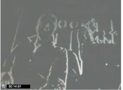
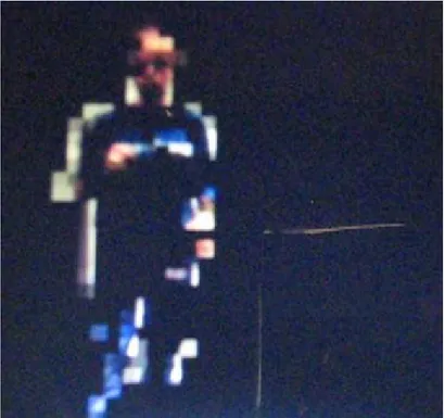
In this chapter the experimental results are presented. Figure 5.13, Figure 5.14 and Figure 5.15 show a sequences of images taken from the LCD screen connected to the WiCa. The white H, L and + represent the the search areas centers of head, left hand and right hand respectively.
The first sequence is relevant for head tracking, indeed the head goes downhill from (1) to (4) and return up from (5) to (8). The second sequence shows the hands crossing. Boxing is displayed in the third sequence.
(1) (2)
(3) (4)
(5) (6)
(7) (8)
(1) (2)
(3) (4)
(5) (6)
(7) (8)
(1) (2)
(3) (4)
(5) (6)
(7) (8)
camera (WiCa) developed by NXP Semiconductor research which combines an SIMD processor (Xetal/IC3D) for low-level operations, an 8051 micro-processor for high-level operations, RAM for inter-frame processing and a ZigBee transmitter for communication.
The algorithm uses different characteristics specific of hands and head in order to identify them during the time. These features are color, edge and motion. Edge and motion allow to represent quite reliable head and hands respectively. Indeed, the face is full of edges and moves slowly while hands move relatively fast and therefore they are blurred so that it is difficult to get sharp, high gradient edges.
We uses thresholds and apply a density function that allows to capture quite reliably hands and head while removing most of the noise (we consider wrong classification of pixels as hands or head noise). The noise is almost absent when skintone is combined with edge density and motion density. In order to track, a search area is defined around each object; the object is followed from frame to frame inside this area.
Each of the features used is affected by the light conditions. In order to make the system more robust, an adaptive thresholding mechanism has been employed. However, the algorithm suffers under non-uniform light conditions especially when there are different sources of light.
The algorithm does not involve the initialization phase, that is hands and head have to be placed in the search areas before starting to track.
2006.
[4] R. Kleihorst, A. Abbo, A. van der Avoird, M. O. de Beeck, L. Sevat, P. Wielage, R. van Veen, and H. van Herten. Xetal: A low-power high-performance smart camera processor, in ISCAS 2001, (Sydney, Australia), may 2001.
[5] P. Jonker. Why linear arrays are better image processors. In Proc.12th IAPR Conf. on Pattern Recognition, (Jerusalem, Israel), pp. 334.338, 1994.
[6] A. M. McIvor. Background subtraction techniques. In Proc. of Image and Vision Computing, Auckland, New Zealand, 2000.
[7] Gonzalez, R. C. and Woods, R. E. [2002]. Digital Image Processing, 2nd ed., Prentice Hall, Upper Saddle River, NJ.
[8] McQueen, J. 1967. Some methods for classification and analysis of multivariate observations. In: Proc. 5th Berkeley Symp. on Math. Statist. Probab., pp. 281-297.
[9] D. Comaniciu, P. Meer. Mean Shift: A Robust Approach toward Fea-ture Space Analysis, IEEE Trans. Pattern Analysis Machine Intell., Vol. 24, No. 5, 603-619, 2002.
work Calibration from Dynamic Silhouettes, CVPR 2004, at Wash-ington DC.
[13] Andrew Barton-Sweeney, Dimitrios Lymberopoulos, Eugenio Culur-ciello and Andreas Savvides, Online camera calibration and node lo-calization in sensor networks, ACM 2005, San Diego, California, USA. [14] Thida, M.[Myo], Chan, K.L.[Kap Luk], Eng, H.L.[How-Lung], An Im-proved Real-Time Contour Tracking Algorithm Using Fast Level Set Method, PSIVT06 2006, 702-711.
[15] Christopher Wren, Ali Azarbayejani, Trevor Darrell, and Alex Pent-land. Pfinder: Real-time tracking of the human body. IEEE Trans. Pattern Analysis and Machine Intelligence, 19(7):780-785, July 1997.
A.1
Proof of 4.8
The equation 4.7 can be written as:
x = α ∗ x + (1 − α) ∗ y (A.1) where in 4.7 fastaverage and blockaverage have been replaced with x and y respectively. Now, it is considered the A.1 frame by frame.
• First frame x1 = α ∗ x0+ (1 − α) ∗ y0 = α ∗ (x0− y0) + y0 (A.2) • Second frame x2 = α ∗ x1+ (1 − α) ∗ y1 = α2∗ (x0− y0) + α(y0− y1) + y1 (A.3) • Third frame x3 = α ∗ x2+ (1 − α) ∗ y2 = α3∗ (x0− y0) + α2(y0− y1) + α ∗ (y1− y2) + y2 (A.4) 56
j=1
Considering 4.5 at frame i+1 (replacing fast threshold with λ) we obtain :
|xi − yi| > λ (A.7)
Taking into account A.6 the term inside the absolute value becomes : xi− yi = αi∗ (x0− y0) +
i−1
X
j=1
αi−j ∗ (yj−1− yj) + yi−1− yi (A.8)
Then A.8 can be written as shown in A.9 (combining the last difference in the sum). xi− yi = αi∗ (x0− y0) + i X j=1 αi−j∗ (yj−1− yj) (A.9)
Supposing that x0 = y0 = 0 (this is reasonable because before the first
frame these values are negligible) then A.7 becomes: |
i
X
j=1
αi−j ∗ (yj−1− yj)| > λ (A.10)
A.10 was presumed before as 4.8 Q.E.D.
A.2
Example of Block-based Background
Sub-traction
This example shows the behavior of the algorithm when an object enters in a block and does not leave anymore. It has been supposed, for simplicity,
Figure A.1: .
The figure A.2 shows how |xi− yi| changes for different values of α. As
can be seen, as α grows, the peak grows and the curve takes more frames to decrease when blockaverage does not change anymore. Every curves reaches the peak as soon as blockaverage reaches its peak, but the peaks values are different. The exact value of the peak can be computed solving |xi − yi| on
the supposition that yj−1− yj = K in 4.8. In fact, we considere simply the
frames in which the blockaverage changes, it is possible to write the 4.8 as shown in A.11 |K ∗ i X j=1 αi−j| > λ (A.11) The summatory inside the absolute operator can be solved as follows:
i X j=1 αi−j = i−1 X m=0 αm = 1 − α i 1 − α (A.12) Thus, the A.11 becomes as in A.13.
Figure A.2: . |K ∗ 1 − α
i
1 − α| > λ (A.13) Therefore, the peak value is given by the left term of the inequation when i is equals to the frames in which blockaverage reaches its maximum value. It is clear the relationship between α, λ (that is fast threshold ) and the blockaverage difference. Figure A.3 shows the behavior for α equals to 0.9 and for different values of K (it was used the same range for the blockaverage values previously used).
Comparing the two Figures A.2 and A.3 it is possible to notice that α decides how many frames are needed to absorb the object in the background when it does not move anymore, while the variation (K in this case) in the blockaverage decides how many frames are needed to reach the peak.
It is interesting to view what happen when an object enters in the block and leaves the block. In this case, it is important to know the number of frames needed to converge below the threshold (i.e. foreground merge into background). The Figure A.4 shows the blockaverage values used for the example (the slope of the leaning curve is K=5). As can be seen, the average start from zero (no moving object in the block) and arrives at 100 (maximum value); after this, the object leaves the block and the average approaches the background value.
Figure A.3: .
j=1
Before the peak of blockaverage, all the differences are negative but after the peak the differences become positive, so that, A.14 starts to decrease. When i (the frame number) is high enough to consider only the descend line, all the differences are positive, that is, A.14 starts to increase. When blockaverage reaches its steady state, A.14 decreases untill zero (how fast it happens depends on the value of α).
B.1
K-means
The code shows below execute the classification procedure basing on the distance from the centroid. This code is carried out for every row of the frame.
d i s t a n c e = abs ( yuv [ 1 ] [ 0 ] − 1 2 8 ) + abs ( yuv [ 2 ] [ 0 ] − 1 2 8 ) ; t e s t [ 0 ] = abs ( yuv [ 1 ] [ 0 ] − u2 ) ; t e s t [ 1 ] = abs ( yuv [ 2 ] [ 0 ] − v2 ) ; c l a s s = ( d i s t a n c e > t e s t [ 0 ] + t e s t [ 1 ] && t e s t [ 0 ] < l i m i t 2 u && t e s t [ 1 ] < l i m i t 2 v ) ? 2 : 0 ;
Every frame the centroid is updated basing on the pixels classified as belonging to the class tracked. To accomplish this step, during the frame the distribution of these pixels in the UV space is computed by exploiting the following code.
u p o s = (
p i d > ( c c e n t e r −dim)>>1 && p i d <( c c e n t e r+dim)>>1 && c l a s s == 2
&& yuv [ 1 ] [ 0 ] > u c e n t e r
&& yuv [ 1 ] [ 0 ] < u c e n t e r + k m e a n s m a r g i n ) ? u p o s+1 : u p o s ;
&& yuv [ 2 ] [ 0 ] > v c e n t e r
&& yuv [ 2 ] [ 0 ] < v c e n t e r + k m e a n s m a r g i n ) ? v p o s+1 : v p o s ;
v p o s = (
p i d > ( c c e n t e r −dim)>>1 && p i d <( c c e n t e r+dim)>>1 && c l a s s == 2
&& yuv [ 2 ] [ 0 ] < v c e n t e r
&& yuv [ 2 ] [ 0 ] > v c e n t e r − k m e a n s m a r g i n ) ? v p o s −1 : v p o s ;
The centroid is updated,at the end of the frame, according to the previous computations as follow.
i n t temp sum ;
temp sum = Sum( u p o s ) ;
i f ( temp sum > k m e a n s t h r e s h o l d ) u c e n t e r ++; i f ( temp sum < −k m e a n s t h r e s h o l d ) u c e n t e r −−; temp sum = Sum( v p o s ) ;
i f ( temp sum > k m e a n s t h r e s h o l d ) v c e n t e r ++; i f ( temp sum < −k m e a n s t h r e s h o l d ) v c e n t e r −−; u2=u c e n t e r ; v2=v c e n t e r ; // k e e p c l u s t e r s i n t h e i r h e m i s p h e r e s u2 = min ( u2 , s t a r t u 2+hemi ) ; u2 = max ( u2 , s t a r t u 2 −hemi ) ; v2 = min ( v2 , s t a r t v 2+hemi ) ; v2 = max ( v2 , s t a r t v 2 −hemi ) ;
B.2
Tracking
In order to track the center of mass of one object, a simple procedure is used. For the x-coordinate it computes the number of pixels that lie to the left and to the right of the center of the square area. It decides the direction
// . . . c t i c = c l a s s == 2 && p i d > ( c c e n t e r −dim ) && p i d < ( c c e n t e r ) ? c t i c −1: c t i c ; // l e f t s i d e c t i c = c l a s s == 2 && p i d > ( c c e n t e r ) && p i d < ( c c e n t e r+dim ) ? c t i c +1: c t i c ; // r i g h t s i d e // . . . } // y−c o o r d i n a t e
i f ( rows > r c e n t e r − dim && rows < r c e n t e r ) { // upper p a r t r t i c = c l a s s == 2 && p i d > ( c c e n t e r −dim ) && p i d < ( c c e n t e r+dim ) ? r t i c −1: r t i c ; }
i f ( rows > r c e n t e r && rows < r c e n t e r+dim ) { // l o w e r p a r t r t i c = c l a s s == 2 && p i d > ( c c e n t e r −dim ) && p i d < ( c c e n t e r+dim ) ? r t i c +1: r t i c ; }
Armed with these quantities, at the beginning of each frame it computes the new position of the object exploiting the code shown below.
i n t s u m t i c = Sum( c t i c ) ;
i f ( s u m t i c > 0 ) c c e n t e r=c c e n t e r+v e l x ; i f ( s u m t i c < 0 ) c c e n t e r=c c e n t e r −v e l x ; s u m t i c = Sum( r t i c ) ;
in Figure 3.2, the input image is sift through a few steps each of which represent a feature. Every step works separately, so that each feature has its own thresholding.
Figure C.1: In-node features extraction parallel scheme : skin-like moving object.
This is not the only approach that can be used. Indeed, in Chapter 3 we gave a hint to the parallel method. Basically, the features are normalized and
move part of the noise. We obtain interesting results applying the adaptive thresholding explained in Chapter 5 to both thresholds (the one for the com-bination of segmentation and motion and the one for the density function).
This approach is really interesting because it produces a more flexible system able to adapt itself at different light conditions. However, the system shown sensibility to the noise so that, it is less reliable compared to the serial system developed during this work.