Analisi di uno scenario di parziale
congelamento del sistema primario
Ivan Di Piazza
Report RdS/2013/028 Agenzia nazionale per le nuove tecnologie,
ANALISI DI UNO SCENARIO DI PARZIALE CONGELAMENTO DEL SISTEMA PRIMARIO
Ivan Di Piazza (ENEA) Settembre 2013
Report Ricerca di Sistema Elettrico
Accordo di Programma Ministero dello Sviluppo Economico -‐ ENEA Piano Annuale di Realizzazione 2012
Area: Produzione di energia elettrica e protezione dell'ambiente
Progetto: Sviluppo competenze scientifiche nel campo della sicurezza nucleare e collaborazione ai programmi internazionali per il nucleare di IV Generazione
Obiettivo: Sviluppo competenze scientifiche nel campo della sicurezza nucleare Responsabile del Progetto: Mariano Tarantino, ENEA
Index
1. Introduction ... 3
2. Numerical Models and methods ... 4
2.1 General Framework ... 4
2.2 Formulation of the Method ... 4
3. Application to a real case ... 6
3.1 The NACIE-UP Heat Exchanger ... 6
3.2 CFD model and boundary conditions ... 10
3.2 Results ... 12
4. Conclusions ... 18
1. Introduction
In the context of GEN-IV Heavy Liquid Metal safety studies, the lead freezing in the pool is considered one of the main issues to be addressed and a realistic accident for a LFR DEMO.
With respect to LWR or to sodium-cooled fast reactors, in Lead cooled fast reactors (LFR) [1] the boiling of the coolant is very unlikely due to the high boiling temperature of Lead (1740 °C). This represents a big advantage of the Lead technology with respect to the other ones. On the other hand, lead freezing temperature is Tfreez∼330 °C and lead is frozen at room temperature. Therefore the lead freezing has to be considered as a possibility, and the safety issues related to scenarios with frozen lead is completely new for nuclear technology and it must be careful investigated.
The consequences of a LEad FReezing Accident (LEFRA) in some part of the lead pool are probably the full damaging (mechanical braking) of the components involved and a serious damaging of the reactor with a big economic and safety impact and this scenario must be considered as extreme. The first components to focus are of course the cold sinks of the pool, i.e. the Steam Generator (SG) and the Decay Heat Removal heat exchangers (DHR). In the case of accident, for example, if the DHR can extract from the system more power than the decay power, the average temperature of the pool can go down and in this case the HX is the first component in which the lead temperature could fall below the freezing temperature.
In this framework, the impact of lead freezing on the system components, on the heat removal and on the global safety of the plant must be addressed very carefully. A program of experiments and numerical studies should be planned in the next future to have a detailed picture of the freezing in LFR pool reactors. This program has not yet planned and both in the literature and in the reports of the European research centers the freezing topic has not been investigated very much.
The present document is a first step towards a detailed analysis of such phenomena, and a CFD model and approach is presented to have a detailed thermo-fluid dynamic picture in the case of freezing. In particular, a numerical methodology is presented to model the freezing of lead and the heat transfer in a proper way.
At this stage, examples are given on the prototypical Shell-and-tube Heat Exchanger of the NACIE-UP facility located at the Brasimone research center. The facility is operated in LBE (lead-Bismuth Eutectic) and the secondary fluid is pressurized water at 16 bar. LBE is characterized by thermo-fluid dynamic properties similar to those of Lead, but the freezing/melting temperature is ∼200°C lower than Lead, i.e. Tfreez∼130 °C.
From the numerical side, the first step towards this investigating program is the definition of the numerical methods and tools to correctly capture the physical phenomena involved. For the Computational Fluid Dynamics (CFD) it is not really convenient to describe the problem as a real two-phase problem with two-phase changing. In fact, in this case the problem formulation and the numerical discretization would be highly complex without probably adding relevant physical information. The simplified approach proposed here allows capturing most of the physics with a much easier formulation and maintaining the one-fluid, one-phase approach. Considering that other sources of errors are present in the CFD modeling (i.e. turbulence models, numerical discretization, geometry
simplifications, etc.) the present proposal is considered by the author by far sufficient to capture the relevant physics.
2. Numerical Models and methods
2.1 General Framework
The general purpose code ANSYS CFX 13 [2] was used for all the numerical simulations presented in this paper. The code employs a coupled technique, which simultaneously solves all the transport equations in the whole domain through a false time-step algorithm. The linearized system of equations is preconditioned in order to reduce all the eigenvalues to the same order of magnitude. The multi-grid approach reduces the low frequency error, converting it to a high frequency error at the finest grid level; this results in a great acceleration of convergence. Although, with this method, a single iteration is slower than a single iteration in the classical decoupled (segregated) SIMPLE approach, the number of iterations necessary for a full convergence to a steady state is generally of the order of 102, against typical values of 103 for decoupled algorithms.
The SST (Shear Stress Transport) k-ω model by Menter [3] is extensively used for the simulations presented here. It is formulated to solve the viscous sub-layer explicitly, and requires several computational grid points inside this latter. The model applies the k-ω model close to the wall, and the
k-ε model (in a k-ω formulation) in the core region, with a blending function in between. It was originally designed to provide accurate predictions of flow separation under adverse pressure gradients, but has since been applied to a large variety of turbulent flows and is now the default and most commonly used model in CFX-13 and other CFD codes. The turbulent Prandtl number in the case of lead or LBE has been fixed to 1.1, according to the suggestion of the literature [4] and to the author’s experience [5] [6].
2.2 Formulation of the Method
To simulate the phase change from the liquid to the solid phase several modifications have been introduced in the code. The modifications have been implemented by the CFX Expression Language (CEL), but the user subroutines could be used as well with similar results.
As already stated in section 1, the single-fluid single-phase approach has been chosen to simulate the freezing phenomena. The basic idea and the main approximation is to consider the freezing process occurring in a small temperature range ∆Tmelt∼1-2 °C (freezing Temperature window) instead that at a constant temperature T=Tfreez~327 °C for Lead or T=Tfreez~124 °C for LBE, i.e. the process is simulated between Tfreez and Tfreez-∆Tmelt. This issue is addressed by setting the specific heat cp in the freezing window much higher that cp in the liquid and in the solid phase. A practical numerical optimizing procedure gave the following values for the specific heat for Lead:
0 146.7 [ / ] p p freez c =c = J kgK for T>T (1) 0 146.7 [ / ] p p freez melt c =c = J kgK for T<T − ∆T (2) 0 100 14600.7 [ / ]
p p freez melt freez
c = ⋅c = J kgK for T − ∆T < <T T (3)
With the above choices the freezing temperature window ∆Tmelt can be computed in a physically consistent way on the base of the freezing latent heat for lead ∆HmeltLead and for LBE ∆HmeltLBE:
23800[ / ] Lead melt H J kg ∆ ≈ (4) 38500 [ / ] LBE melt H J kg ∆ ≈ (5) 0 1.63[ ] 100 Lead Lead melt melt p H T C c ∆ ∆ = ≈ ° ⋅ (6) 0 2.62[ ] 100 LBE LBE melt melt p H T C c ∆ ∆ = ≈ ° ⋅ (7)
∆Tmelt is in the correct range stated above and would lead to an acceptable approximation of the real physical behaviour. These modifications will introduce an ‘energetic’ behaviour similar to the real fluid because when the fluid temperature reaches the freezing temperature Tfreez, the unit mass of fluid will be in the freezing temperature windows until it will provide to the neighbours exactly the energy ∆Hmelt.
The second step towards a full formulation of the problem is to implement the mechanical behaviour of the fluid during the phase change and in the solid phase. The idea is to introduce a force which simulates the growing resistance of the fluid during solidification and which stops completely the fluid motion in the solid phase. This is done by the use of proper source terms in the momentum equation. In each direction (x,y,z) , a drag negative source term is chosen proportional to the velocity in that direction (u,v,w), according to the expressions:
( ) u S = −C T ⋅u (8) ( ) v S = −C T ⋅v (9) ( ) v S = −C T ⋅w (10)
The source term must be expressed in N/m3, i.e. in kg/m2s2, and therefore the function C(T) is expressed in kg/m3. The function C(T) is chosen in a proper way to be 0 in the liquid range and very high in the solid range, with a linear behaviour in the freezing window.
Introducing the solid fraction γ, which represents the frozen fraction of the unit mass in the freezing window: melt freez T T T γ = − ∆ (11)
The specific value set to ensure numerical convergence to the code and a suitable mechanical behaviour of the fluid in the melting window are expressed by the following formulas:
3
( ) 0 [ / ] freez
5 3 1
( ) 10 [ / ] freez melt
C T =C = kg m for T <T − ∆T (13)
1
( ) freez melt freez
C T = ⋅C γ for T − ∆T < <T T (14)
This formulation ensures a realistic behaviour, because the resistance to the flow circulations grows with the solid fraction, although the physical consistent form of the constant in the freezing window (Eq. 14) should be assessed by proper experimental data. The high value of the constant in the solid region (Eq. 13) ensures that the velocity is practically 0 for T<Tfreez-∆Tmelt.
The whole formulation is completely auto-consistent and guarantees that the correct heat transfer mechanisms can take place. In the liquid range, for T>Tfreez, the set of the equations to solve is that of an ordinary single-phase flow; in the solid range, for T<Tfreez-∆Tmelt, the convective terms are negligible and the heat transfer is governed by conduction; in the freezing windows, Tfreez-∆Tmelt <T<Tfreez, the convective terms decreases while the solid fraction increases.
The global temperature distribution and the energy balance is completely physically-consistent because the freezing window is tied to the freezing latent heat ∆Hmelt.
3. Application to a real case
3.1 The NACIE-UP Heat Exchanger
The general method illustrated in section 2.2 is now applied to a low power section of the Heat Exchanger of the NACIE-UP loop located at the ENEA Brasimone R.C..
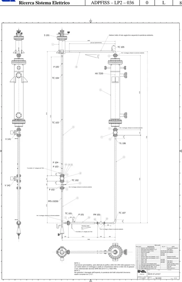
A schematic layout of the primary side of the facility is reported in Figure 1. The facility includes: The Primary side, filled with LBE, with 2 ½” pipes, where the main new components and instruments will be placed:
A new Fuel Pin Simulator (19-pins) 250 kW maximum power;
A new Shell and tube HX with two sections, operating at low power (5-50 kW) and high
power (50-250 kW);
A new low mass flow rate induction flow meter (0-3 kg/s) FM101;
A new high mass flow rate induction flow meter (3-15 kg/s) FM102;
5 bubble tubes to measure the pressure drops across the main components and the pipes; Several bulk thermocouples to monitor the temperature along the flow path in the loop;
The Secondary side, filled with water at 16 bar, connected to the HX, shell side. It includes a pump, an air-cooler, by-pass and isolation valves, and a pressurizer (S201) with cover gas; An ancillary gas system, to ensure a proper cover gas in the expansion tank, and to provide gas-lift enhanced circulation;
The ancillary gas system is practically identical to the previous configuration of the NACIE facility and does not have significant upgrade. It has the function to ensure the cover gas in S101 and to manage the gas-lift system in the riser (T103) for enhanced circulation regime.
The primary system is ordinary filled with liquid LBE and it is made by several components, pipes and coupling flanges. Pipes T101, T103, T104, T105 are austenitic SS AISI304 2.5ʺS40, I.D. 62.68 mm. The secondary side is a 16 bar pressurized water loop, with a circulation pump.
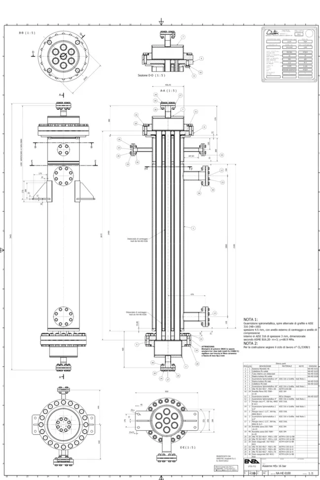
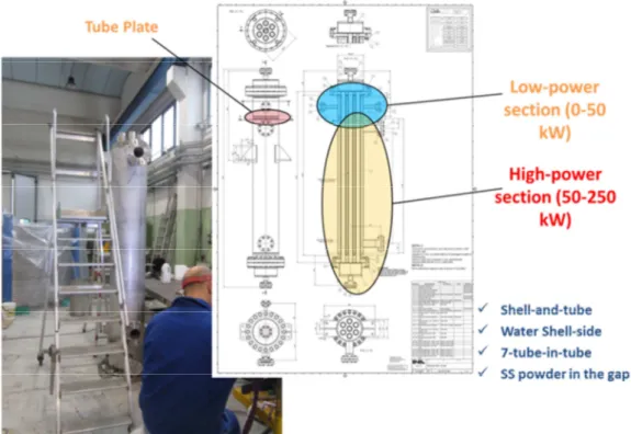
The heat exchanger has been designed to exchange heat up to 250 kW. It is designed as a shell and tube HX with pressurized water (16 bar) on the shell side and LBE on the tube side. ENEA has implemented the tube-in tube concept with stainless steel powder in the gap, to mitigate thermal stresses in the HX and to test the safety concept. An overall layout of the component is reported in Figure 2 while a picture and a schematic indication of the parts are reported in Figure 3. Two separated shell sections have been realized: a counter-current high-power section (30-250 kW) and a cross-flow low power section (0-30 kW), both connected to the pressurized water secondary side. The secondary mass flow rates and temperatures in different conditions have been obtained by CFD computations, but the real operational working table will be addressed on the basis of the real practical experience.
The two sections can be drained and filled separately, and thus the transition from high-power to low-power can be carried out in the NACIE-UP loop. A PID system will allow to control the temperature on the secondary side and the secondary mass flow rate separately.
3.2 CFD model and boundary conditions
The cross-flow low power section (30-250 kW) of the HX has been modelled in this context. The model reproduce the real geometry of the internal chamber of the HX and it includes the shell water side, the LBE tube side, the internal and external SS tubes and the powder gap. These last three structures are treated as solid which transmit power by conduction, while the Navier-Stokes equations with turbulence model have been solved in the water and LBE domain. Therefore the 3D conjugate heat transfer problem is fully addressed.
A perspective view of the computational domain modelled is shown in Errore. L'origine riferimento
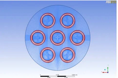
non è stata trovata., while a top view is shown in Figure 5. The top view in Figure 5 evidences the
pipe and powder gap thermal structures, and the secondary water inlet and outlet.
Adiabatic conditions have been imposed on the shell internal walls, and pressure conditions have been imposed at the outlets both for water and LBE. Mass flow rate (m&inw,m&inLBE) and temperatures (Tinw,
LBE in
T ) have been imposed at the water and LBE inlets, and these latter parameters actually controls the heat transfer and the freezing phenomena.
The computational mesh is fully structured and solves the mechanical and thermal boundary layer both for water and LBE with y+~1 at the walls. The mesh in the middle section is shown in Figure 6.
Figure 4 Heat Exchanger domain modelled by CFD: perspective view.
3.2 Results
Several test cases have been run in order to find the conditions that lead to LBE freezing inside the pipes. The test matrix with boundary conditions is reported in Table 1 and the mass flow rates both for water and LBE are consistent to what can be operated in the facility in the next experimental campaigns.
The full convergence has been reached in all cases with residuals of the equations below 10-6.
Table 1 Test matrix for freezing calculation is the NACIE-UP HX.
CASE LBE
in
m& [kg/s] TinLBE[°C] m&inw [m3/h] Tinw [°C] Freezing
11 2 200 10 150 NO
12 2 250 10 40 NO
13 2 250 10 20 YES
14 2 225 10 20 YES
15 2 200 10 20 YES
For case 11 freezing is not expected and it is not found because the water inlet temperature (
150
w in
T = °C) is larger than the LBE freezing temperature of 124 °C. Case 11 corresponds to a normal operational case of the HX and shows results in line to what expected with a total power exchanged
Q~6.5 kW. The temperature distribution at the pipe wall in contact with water is quite uniform with
variation of about 10 °C, as shown in Figure 7.
For the cases from 12 to 15, the hypothesis is that, for some reason, relatively ‘cold’ water enters in the HX and thus the heat exchange phenomena are strongly influenced with the possibility of LBE freezing.
In case 12, the water temperature is 40 °C and this is not sufficient to cause LBE freezing. For cases 13 to 15, the freezing occurs and the occlusion is progressively larger.
In the next figures, case 15 will be presented in details and finally a comparison will be carried out between all different cases.
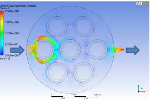
Figure 8 shows the vector plot in the water shell in the z midplane; the color code represents the velocity module. A typical cross-flow develops with lots of recirculation regions and an impinging region in the tube in front of the water inlet.
Figure 7 Temperature distribution in the wall in contact with water for case 11.
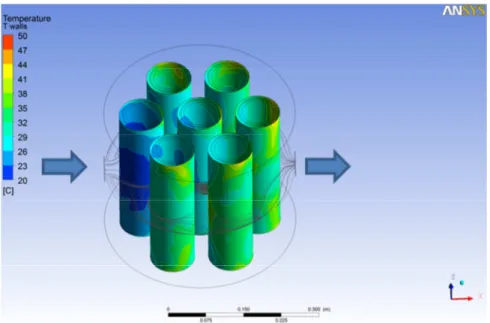
Figure 9 shows the temperature distribution in the wall in contact with water for case 15. In this case the temperature disuniformity is larger than for case 11, due to the larger temperature difference between LBE and water. The minimum temperature (20 °C) are located in the impinging region of the tube closer to the water inlet, while the maximum temperatures (~40-50 °C) are located in the recirculation regions in the top part of the shell, in correspondence to the LBE inlet.
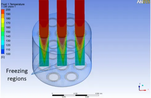
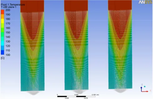
Figure 10 shows the temperature distribution in a x-z plane which includes the water inlet-outlet sections. The temperature in the LBE shows that values below the freezing temperature (124 °C) are present close to the pipe outlet region. This fact is better evidenced by Figure 11 in which the only LBE temperature is reported with a proper scale.
Figure 12 shows the corresponding streamwise velocity contours in LBE for case 15. The model of the freezing actually leads to the ‘red’ regions close to the wall where the velocity is practically zero. Figure 13 shows a zoom of the temperature contours in a x-z plane in LBE outlet region with velocity vector superimposed for the same case. It can be noticed how the model guarantees a smooth transition between liquid LBE and solid LBE close to the wall.
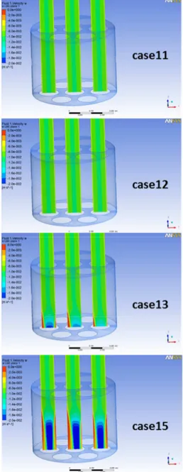
Figure 14 shows a comparison between streamwise velocity contours in the LBE for cases 11, 12, 13 and 15. Cases 13 and 15 are characterized by a different degree of freezing and show that the phenomena can be modeled in any case.
Figure 10 Temperature contours in a x-z plane for case 15.
Figure 12 Streamwise w velocity contours in LBE for case 15.
4. Conclusions
A CFD method is presented to simulate fluid flow and heat transfer during solidification of Lead or Lead Bismuth Eutectic (LBE) in any geometry. The method allows formally maintaining a single-phase approach introducing momentum source terms depending on local velocity and temperature dependent specific heat. The global physical consistence of the method is guaranteed by the fact that the melting latent heat is correctly kept into account in the formulation. In the fully frozen regions the velocities are 0 and the transport of heat is governed by the thermal conductivity. Where the solid fraction is between 0 and 1, the convective terms are dumped according to the specific form of the momentum source term.
The method has been applied successfully to a real component, i.e. the Heat Exchanger of the NACIE-UP facility located at the ENEA Brasimone R.C.. The method provided fully converged results in any conditions and can include conjugate heat transfer in the thermal structures and other physical effects ordinary modeled by CFD. The cases presented are realistic and they are provided to show the global consistency and robustness of the method. The full feasibility of the method is proved, and the lead freezing has been obtained in the CFD simulation in the regions where it was expected by physical intuition. The model can guarantee a smooth transition between liquid metal and frozen metal.
The next step towards a full assessment of the method is to find a more accurate form of the source terms in the melting regions by comparison with experimental data. Afterword, the method can be applied to any system. To do this, an experimental facility called SOLIDX has to be designed, built and instrumented at the Brasimone R.C.. The conceptual design of the facility is ongoing. The investigation domain of the facility will be a cavity filled by LBE or Lead in natural circulation, and acoustic techniques will be adopted to measure the thickness of the frozen LBE in the cold wall. This will allow to set the model constants properties and to check if the numerical model provides accurate results compared with the experiments both in laminar and turbulent flows.
5. References
[1] A. Alemberti, J. Carlsson, E. Malambu, A. Orden, D. Struwe, P. Agostinif, S. Monti, European lead fast reactor—ELSY, Nucl Eng Design, 241, pp.3470-3480, 2011.
[2] ANSYS CFX Release 13 User Manual.
[3] F. R. Menter, Two-equation eddy-viscosity turbulence models for engineering applications,
AIAA J, 32, pp.269-289, 1994.
[4] X. Cheng, N.I. Tak, CFD analysis of thermal-hydraulic behavior of heavy liquid metals in sub-channels, Nucl Eng Design, 236, pp.1874-1885, 2006.
[5] I. Di Piazza, M. Scarpa, Rassegna di Letteratura sulla Termoidraulica dei Bundle Refrigerati a Metallo Liquido Pesante, ENEA Report LM-FR-001, 2012.
[6] M. Scarpa, CFD Thermal Hydraulic Analysis of HLM cooled rod bundles, Master Thesis Univ. of Pisa, Italy, 2013.