Probabilistic Envelope Curves for Extreme Rainfall Events - Curve Inviluppo Probabilistiche per Precipitazioni Estreme

FACOLTA’ DI INGEGNERIA

Corso di Laurea in Ingegneria per l’Ambiente e il Territorio

Insegnamento di Costruzioni Idrauliche e Protezione Idraulica del Territorio DISTART - Dipartimento di Ingegneria delle Strutture, dei Trasporti, delle Acque,

del Rilevamento, del Territorio

PROBABILISTIC

ENVELOPE

CURVES

FOR

EXTREMES

RAINFALL

EVENTS

CURVE

INVILUPPO

PROBABILISTICHE

PER

PRECIPITAZIONI

ESTREME

Anno Accademico 2006/2007 Sessione III

TESI DI LAUREA DI: RELATORI:

Lorenza Tagliaferri Chiar.mo. Prof. Ing. Armando

Brath

Chiar.mo Prof. Ing. Günter Blöschl

CORRELATORI: Dott. Ing. Ralf Merz

Parole Chiave: •Analisi di frequenza •Austria •Italia •Precipitazioni estreme •Curve inviluppo

Water is an image of the evolution and the cycle of life and flows over borders and breaks limits. A genuine symbol against all preconceived tracks.

I

NDEX

INTRODUZIONE... 7

1 INTRODUCTION ... 10

2 METHODOLOGIES FOR THE DESIGN FLOOD ESTIMATION ... 14

2.1 INDIRECT METHODS... 16

2.2 ESTIMATION OF THE DESIGN RAINFALL EVENT... 17

2.3 OTHER FLOOD ESTIMATION METHODS... 19

3 FREQUENCY ANALYSIS OF EXTREME EVENTS ... 20

3.1 PROBABILITY CONCEPTS... 20

3.2 PROBABILITY DISTRIBUTIONS FOR EXTREME EVENTS... 24

3.2.1 The Normal Distribution ... 24

3.2.2 The Lognormal Distribution ... 26

3.2.3 The Gumbel Distribution ... 27

3.2.4 The Generalized Gumbel Distribution (GEV)... 32

3.2.5 The Weibull Distribution... 34

3.3 PLOTTING POSITIONS AND PROBABILITY PLOTS... 34

3.3.1 Choice of Plotting Position ... 35

4 PROBABLE MAXIMUM PRECIPITATION ... 38

5 PROBABILISTIC ENVELOPE CURVES FOR EXTREME FLOODS ... 40

5.1 DEFINITION OF REGIONAL ENVELOPE CURVES... 40

5.2 APROBABILISTIC INTERPRETATION OF ENVELOPE CURVES... 43

5.3 DESCRIPTION OF THE METHOD... 43

5.3.1 Estimating the Effective Number of Sites ... 44

5.3.2 Evaluation of the Intersite Correlation ... 45

5.3.3 Estimating the Effective Sample Years of Data... 46

6 STUDY REGIONS AND LOCAL REGIME OF RAINFALL EXTREMES ... 48

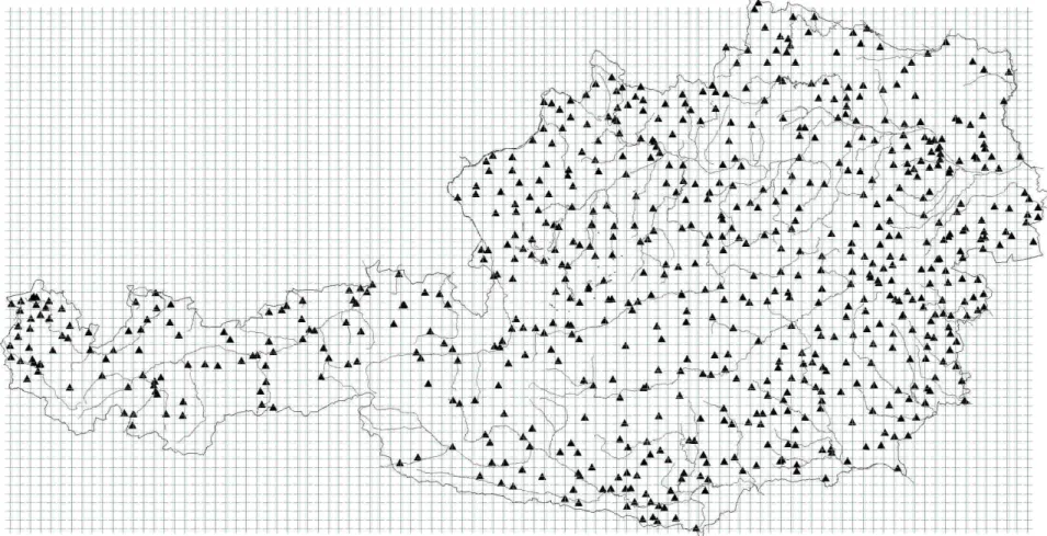
6.1 CLIMATE AND MORPHOLOGY OF AUSTRIA... 48

6.2 AVAILABLE RAINFALL DATA... 52

6.2.1 Peaks-Over-Threshold Procedure ... 53

6.2.2 Identification of Regions ... 55

6.4 AVAILABLE RAINFALL DATA... 63 7 METHODOLOGY... 65 7.1 AUSTRIAN CATCHMENTS... 65 7.1.1 Uncorrelated Case ... 66 7.1.2 Correlated Case ... 68 7.2 ITALIAN CATCHMENTS... 73

7.2.1 Analysis and Modelling of Intersite Correlation... 78

7.2.2 Validation Procedure... 84

8 DISCUSSIONS AND CONCLUSIONS ... 86

CONCLUSIONI... 89

APPENDIX... 92

ANNEXES... 94

REFERENCES... 119

I

NTRODUZIONE

Gli eventi naturali estremi, quali portate di piena, siccità, forti piogge, mareggiate, terremoti o venti di particolare intensità, possono generare conseguenze catastrofiche per l’uomo e per la società. E’ pertanto evidente come la stima della frequenza di accadimento di un particolare evento sia un problema di grande importanza ed interesse scientifico.

Le attività di pianificazione e controllo di emergenze climatiche, le attività di protezione civile, il progetto di strutture di ingegneria civile, la gestione delle riserve naturali, il controllo ambientale e il calcolo per la protezione da rischi ambientali si fondano in buona misura sulla conoscenza del regime di frequenza di eventi estremi. La stima di tali frequenze non risulta però agevole in quanto gli eventi estremi sono rari per definizione e la loro osservazione è assai sporadica, a ciò va sommato il fatto che molto spesso le serie storiche disponibili hanno lunghezza assai limitata.

In particolare la valutazione di eventi pluviometrici di progetto è una problematica che desta molto interesse nell’idrologia. La comunità scientifica negli ultimi anni, ha dedicato numerosi sforzi alla messa a punto di tecniche affidabili, per la stima di portate fluviali o di altezze di precipitazione aventi assegnato livello di rischio.

Gli eventi idrologici di progetto (ad esempio portate e precipitazioni) rappresentano ipotetici eventi associati a una data probabilità di superamento, in genere espressa in termini di tempo di ritorno. Per esempio, l’informazione relativa alla portata di progetto è necessaria al fine di identificare le misure di protezione del territorio e delle costruzioni idrauliche dal rischio di esondazione.

Per quanto riguarda le portate estreme la letteratura documenta la diffusa utilizzazione di curve inviluppo regionali (RECs). Tali curve riassumono l’attuale limite di portate estreme verificatesi in una data regione. L’idea di limitare le portate sperimentate tramite una curva inviluppo è classica nell’ambito dell’idrologia e, per gli Stati Uniti, si rifà a Jarvis (1925), che presentò una REC basata sulle portate registrate su 888 siti

Solo 50 anni più tardi, Crippen e Blue, 1977, e Crippen, 1982 aggiorono lo studio fatto da Jarvis nel 1925 creando 17 diverse REC, una per ogni diversa regione idrologica statunitense, basate su un totale di 883 siti. Matalas, 1997 e Vogel, 2001 hanno mostrato come le REC identificate da Crippen e Blue, 1977, e Crippen, 1982 rappresentino il limite delle portate estreme anche nel periodo che va dal 1977 al 1994 per 740 dei 883 siti analizzati da Crippen e Blue.

Enzel et al., 1993 esaminarono le serie storiche di portate limitate da una REC per il bacino del fiume Colorado e videro che la stessa REC corrispondeva anche al limite delle stime delle paleo-portate disponibili per il bacino.

Lo sviluppo e la costruzione delle RECs non è rimasto confinato agli Stati Uniti; sono state sviluppate per l’ Italia (Marchetti, 1955), per la Grecia occidentale (Mimihou, 1984), per il Giappone (Kadoya, 1992) e per altre regioni. Le RECs sono state usate per confrontare le portate manifestatesi negli Stati Uniti, in Cina e nel mondo da Costa, 1987 e, più recentemente, da Herschy, 2002.

Le RECs hanno continuato ad essere costruite e viste soprattutto quali resoconto delle portate manifestatesi, piuttosto quali strumento conoscitivo per il progetto di misure di tutela nei confronti di portate “catastrofiche”. Si pensava che non ci fosse la possibilità di associare a una REC un valore di probabilità (Crippen e Blue, 1977; Crippen, 1982; Vogel et al., 2001).

Water Science and Technology Board, Commission on Geosciences, Environment and Resources (1999) sancirono che la determinazione della probabilità di superamento di una REC era difficile principalmente a causa della correlazione spaziale tra i siti. Di conseguenza le REC non avevano grande utilità nonostante l’ U.S. Interagency Advisory Committee on Water Data (1986) ne riconobbero la necessità per “mostrare e riassumere i dati di portata estremi attualmente in accadimento”.

Sarebbe pertanto interessante fornire un’interpretazione probabilistica di una REC, considerato anche il fatto che negli 80 anni passati da quando Jarvis (1925) ha proposto una curva inviluppo, nessuna interpretazione probabilistica è mai stata presa in esame.

Le precipitazioni costituiscono la componente del ciclo idrologico che maggiormente concorre alla formazione del deflusso superficiale, pertanto lo studio del loro regime di frequenza è un requisito essenziale per valutare il rischio idrogeologico in una determinata regione.

Scopo del presente lavoro di Tesi è l’estensione dell’interpretazione delle curve inviluppo probabilistiche agli eventi di precipitazione estremi, nei bacini italiani e austriaci. Il primo obiettivo dello studio consiste nell’identificazione di un’affidabile metodologia di valutazione, che ci consenta di fornire la stima accurata, in una regione precisa, dell’altezza di precipitazione relativa ad una data durata e posizione, per un assegnato tempo di ritorno, elevato o molto elevato.

In particolare tale analisi punta l’attenzione sulle curve inviluppo regionali, già sviluppate per le portate da Castellarin et al. (2003 e 2007). Gli autori hanno sviluppato uno stimatore empirico del tempo di ritorno T associato a una determinata REC che, il linea di principio, consente l’utilizzo delle RECs a fini ingegneristici di progetto in bacini strumentati e non.

Il seguente lavoro propone l’estensione del concetto di REC agli eventi estremi di precipitazione introducendo la Curva di Durata-Altezza di precipitazione (DDEC), definita come il limite superiore regionale di tutti gli eventi meteorici registrati per diverse durate di precipitazione (qui i dati rappresentano massimi annuali).

Si adatterà inoltre l’interpretazione probabilistica proposta per le REc alle DDEC e all’adattamento di tali curve per la stima dell’evento di pioggia corrispondente ad un elevato tempo di ritorno T e a una assegnata durata.

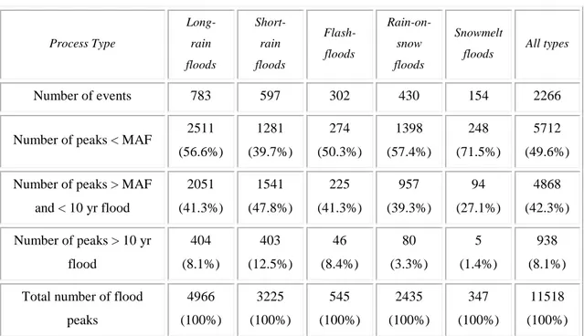
Saranno due i datasets nazionali considerati, la serie di picchi di precipitazione al di sopra di una soglia (POT) per le durate di 30 minuti, 1, 3, 6, 9, 12 e 24 ore ottenuti da 700 stazioni di registrazione in Austria, e le serie dei massimi annuali (AMS) per gli eventi meteorici di durata compresa tra i 15 minuti e le 24 ore raccolti da 220 stazioni di registrazione nell’ Italia centro-settentrionale.

L’approccio alla REC proposto sarà diverso per le due distinte regioni, così come saranno diverse le modifiche apportate al metodo per la stima empirica della probabilità di superamento p.

1

INTRODUCTION

Extreme environmental events, such as floods, droughts, rainstorms, and high winds, may have severe consequences for human society. How frequently an event of a given magnitude may be expected to occur is of great importance. Planning for weather-related emergencies, design of civil engineering structures, reservoir management, pollution control, and insurance risk calculations, all rely on knowledge of the frequency of these extreme events. Estimation of these frequencies is difficult because extreme events are rare by definition and, therefore, available information are often very sparse or short.

In particular the evaluation of extreme design hydrological events is a fundamental and highly debated topic in hydrology. The scientific community gave great importance to the optimization of reliable techniques for the estimation of extreme rainfall events and resulting floods in the last decades.

Design hydrological events (e.g., floods and rainstorms) are hypothetical events associated with a given exceedance probability, generally expressed in terms of recurrence interval. For instance, design flood information is needed for the identification of flood protection measures in a river basin and the design of the related structures, such as levee systems that need to be designed in order to prevent failure or overtopping (hydrologic failure). Design floods are also required for planning measures and structures as well as for safety control of existing structures.

Concerning extreme floods, the literature documents the diffuse utilization of regional envelope curves (RECs). These curves summarize the current bound on our experience of extreme floods in a region. The idea of bounding our flood experience with an envelope curve is classical in hydrology and, for Unites States dates back to Jarvis [1925], who presented a REC based on record floods at 888 sites in the conterminous United States. Roughly 50 years later, Crippen and Bue, 1977 and Crippen, 1982 updated the study by Jarvis, 1925 by creating 17 different RECs, each

for a different hydrologic region within the United States, based on a total of 883 sites. Matalas, 1997 and Vogel et al., 2001 document that the

RECs identified by Crippen and Bue, 1977 and Crippen, 1982 still bound our flood experience gained from 1977– 1994 at 740 of the 883 sites compiled by Crippen and Bue. Enzel et al., 1993 examine the REC bounding the historical flood experience for the Colorado river basin and show that the same REC also bounds the paleoflood discharge estimates available for the basin.

The construction of RECs is not confined to the United States; they have been developed for Italy (Marchetti, 1955), western Greece (Mimikou, 1984), Japan (Kadoya, 1992), and elsewhere. RECs have been used to compare record flood experience in the United States, China, and the world by Costa, 1987 and, more recently, by Herschy, 2002.

The REC provides an effective summary of our regional flood experience. The pioneering work of Hazen, 1914, who formalized flood frequency analysis, a formalism still in use, and who was among the first to suggest a method for improving information at a site through the transfer of information from other sites (i.e., substitution of space for time), has tempered the use of a flood magnitude as a design flood without an accompanying probability statement. Our objective is to provide a probabilistic interpretation of the REC. In the almost 80 years since Jarvis [1925] introduced the envelope curve, a probabilistic interpretation of a REC has never been seriously addressed.

RECs have continued to be constructed and viewed mainly as summary accounts of record floods, rather than as meaningful tools for the design of measures to protect against ‘‘catastrophic’’ floods. It has been suggested that there is no obvious way to assign a probabilistic statement to a REC (see, e.g., Crippen and Bue, 1977; Crippen, 1982; Vogel et al., 2001). Water Science and Technology Board, Commission on Geosciences, Environment and Resources (1999) argued that the determination of the exceedance probability of a REC is difficult due to the impact of intersite correlation. As a consequence, RECs are assumed to have little utility beyond the suggestion of the U.S. Interagency Advisory Committee on Water Data (1986) that they are useful for ‘‘displaying and summarizing data on the actual occurrence of extreme floods.’’ A probabilistic interpretation of the REC offers opportunities for several engineering

applications which seek to exploit regional flood information to augment the effective record length associated with design flood estimates.

A potential advantage of assigning a probabilistic statement to a REC is that this approach avoids the need to extrapolate an assumed at-site flood frequency distribution hen estimating a design event.

Rain is the most important component of the water cycle with respect to the formation of runoff for a wide portion of European climates, the analysis of its frequency regime is fundamental for the assessment of flooding potential of a given area.

Aim of this work is the extension of the probabilistic interpretation of regional envelope curves to extremes rainfall events in Italian and Austrian catchments. The primary objective of the present study is the identification of a reliable methodology that enables us to accurately evaluate the rainfall depth for a given duration and location associated with high and very high recurrence intervals.

In particular this study focuses on probabilistic regional envelope curves proposed by Castellarin et al., (2005) and Castellarin (2007) for flood flows. The authors formulated an empirical estimator of the recurrence interval T associated with a given REC, which, in principle, enables us to use RECs for design purposes in ungauged basins.

This work extends the REC concept to extreme rainstorm events by introducing the Depth-Duration Envelope Curves (DDECs). DDECs are defined as the regional upper bounds on all the record rainfall depths at present for various rainfall duration (here record indicates historical maxima). It also adapts the probabilistic interpretation proposed for RECs to DDECs and it assesses the suitability of these curves for estimating the T-year rainfall event associated with a given duration and large T values

The study focuses on two different national datasets, the peak over threshold (POT) series of rainfall depths with duration 30 minutes, 1, 3, 6, 9 and 24 hours obtained for 700 Austrian raingauges and the Annual Maximum Series (AMS) of rainfall depths with duration spanning from 15 minutes to 24 hours collected at 220

raingauges located in northern-central Italy. The approach to the REC is different for the two catchments as well as the adjustment of the empirical estimator for the exceedance probability p.

2

METHODOLOGIES FOR THE

DESIGN FLOOD ESTIMATION

This paragraph aims to presenting the possible methodologies for the design-flood estimation. This task, as already mentioned, is fundamental in the evaluation of hydrologic risk, and in particular, of flooding potential of a given site.

Both floods and rainfall data can be used as hydrological variables for the estimation of the design flood. The identification of an hydrological variable is developed by two different methodologies, the direct methods that directly calculate the floods and the indirect methods that identify the rainfalls to be given as input in a rainfall-runoff model, able to convert the rainfalls into floods thanks to appropriate calibrations.

Although this work gives particular attention to rainfall events, we are going to illustrate the common methodologies for the design flood estimation.

A common approach for estimating design flood consists of modeling hydrological events as random variables, allowing the determination of the flood exceeded with given probability. Usually the problem is that of information: if one had a sufficiently long record of flood flows, rainfall, low flows or pollutant loadings, then a frequency distribution for a site could be precisely determined, so long as change over time due to urbanization or natural processes did not alter the relationship of concern. In most situations, available data are not sufficient to precisely define the risk of large floods, rainfall, pollutant loadings or low flows.

A fundamental step for the identification of a design event is the evaluation of the relation x = x(T). Then the design event is identified by selecting the return period T believed to be adapt to the importance of the structure itself and to the implications that its failure would involve.

The direct methods determine the expression x = x(T), from the available rainfall data analysis in neighbourhood catchments, otherwise from the extrapolation of

statistical analysis known for neighbourhood catchments, similar from the hydrological point of view.

The indirect methods derive the same expression from the statistical analysis of the extreme rainfall events occurring in the hydrographical catchment, applying later a transformation of these rainfall events in superficial runoff, that means they evaluate the design flood from extreme rainfall events.

The choice between the two methods can be made according to the reliability and validity of the available rainfall data. The use of direct methods requires hydrometrical observations of annual maxima floods for a sufficiently long period of time; this information is later analysed by statistical techniques in order to indentify the probability distribution that better represents the collected data. As described direct methods seem to be the more suitable for their validity and simplicity in application: the variable on which the measurement are mead is the flood itself that is the variable to be estimate for design purposes.

In practical the problem stands in their application: measures are often uncertain or related to hydrometric sections different from that of design, thus their utilization requires extrapolations and hypothesis not easy to formulate.

Moreover, rarely it is possible to arrange sufficiently long flood data sets (20-30 years) able to allow the analysis of return periods connected with the design. If is T larger than the mean length of the available series, the error in the corresponding flood estimation can be significant and consequentially the extrapolations became to have uncertain reliability (it would be better not to have estimations of T greater than 2-3 times the series length (Cunnane, 1986)). Series of limited length can be represented by different probability distributions, from which the obtained extrapolations are very different.

As said, a possible alternative is the recurs to the indirect methods which, based on the rainfall-runoff transformation, are strong of the statistical distributions of the rainfall data, much more than the hydrometrical data. Anyway, the transformation of the design rainfall event in design flood needs the formulation and estimation of model parameters which have the aim of simulating soil infiltration, storage in surface and interception by vegetation. Such complex models introduce great

uncertainty being a rough approximation of realty. It is for this reason important, for the using of indirect methods, the accurate knowledge of the hydrological characteristics of the analysed catchment.

Definitely, the indirect methodology has the power of being correct for a great number of cases, much more than the direct methods, thank to the density of the rainfall net. This typology presents all the same some limiting factors:

• The difficult in arranging sufficient rainfall data for the calibration of the rainfall-runoff model, model that can be very complex;

• Supposing the same frequency for rainfall events and floods, the method gives the same probability to floods and rainfall events, assumption that can be criticised;

In spite of these critics, the indirect one is by now a valid methodology, fundamental for drainage systems and hydrographical nets.

Next paragraph focuses on the indirect methodology.

2.1

I

NDIRECT

M

ETHODS

A different approach is to view flood flows as the product of a deterministic transformation of rainfall events, seen as random variables. Because is rain cause of floods, it is also supposed to be strictly related to them.

The consequent transformation of rainfall in floods will then entrusted to rainfall-runoff models. Several are the typologies of models, all able to represent hydrological phenomena that make the basin as a deterministic system by which rainfall events and floods becomes inputs and outputs.

Different models can be distinguished according to the applied transformation model (event-based or continuous simulation) and to the way the design rainfall event is represented.

We will focus on this representation of rainfall events, without giving importance to the rainfall-runoff simulation.

2.2

E

STIMATION OF THE

D

ESIGN

R

AINFALL

E

VENT

Input to a rainfall-runoff model can be design hyetographs, historical series of rainfall data, or synthetic series of rainfall events generated by stochastic rainfall models: each input is connected to a different probabilistic structure thus a different bond between x and T. According to the defined input indirect methods can be classified as:

• Methods based on depth-duration-frequency curves

• Methods derived by simulation

• Analytic-derived methods

The first ones consist of using a single event model as input to the rainfall-runoff model; these give the bond between the rainfall depth h with occurrence period T and duration t, and the duration t itself. These methods can be found by statistical interference methods by the analysis of the extreme historical series in the neighbourhood of the region of concern. Data are supplied by the National Hydrographical Service of Italy (SIMN) that provide series of maximum rainfall depth data for durations of days or less than a day. For each duration are estimated the parameters of the suitable probability distribution, so to identify the correct quantiles of rainfall depth. Rainfall depths for durations different from the estimates ones, will be calculated by interpolation of the obtained data.

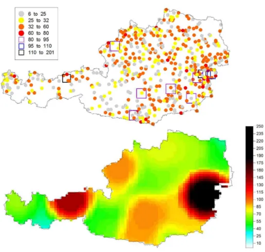
Some other lows are useful for expressing this expression, in Italy we find an exponential relation that describes the grow of the expected rainfall in a certain site with the growing of the duration t, function of the return period T:

h(t,T) = aT ·t

n_T

(2.2-1)

where h represents the rainfall depth, and aT and nT are the parameters to be estimates as function of the return period.

Figure 2.2-1 shows that equation (2.2-1) assumes a convex exponential form on a t/h graph, actually for a given frequency the rainfall rate decreases with duration and the cumulative rain also progressively decreases whit the duration itself.

Figure 3.2.1-1 Representation of the rainfall depth versus duration for different values of return period, it is easily recognizable a convex exponential form

Limit of this method is that for each single site is important to define a depth-duration-frequency curve that require the estimation of many parameters: two parameters for each duration, and two for deriving the exponential law. Considering that the length of the series and the available data are not sufficient, usually smaller than 50-60 years of registration, the estimation of the parameters is not possible.

In order to supply the lack of information, some simplifications can be introduced. For example an constant scale that means rainfall depth for the duration t equal to one corresponding to a given duration, simply multiplied by an estimated scale factor. Although this assumption, not always applicable and to be verified, there is the problem of obtaining rainfall data for ungauged basins: we need a more general expression applicable on regional scale. The introduction of envelope curves let the extension of information to ungauged basins, in the next paragraphs this concept will be studied in depth.

Methods derived by simulation use the rainfall data for a limited number of years to generate, by appropriate rainfall stochastic models, synthetic rainfall series of greater dimensions to be used as input in rainfall-runoff models that give as output

simulated series of floods. By applying to these series the usual statistical techniques we will obtain estimations of design floods. Definitely the design flood is estimated by a simulated series of rainfall data, not really observed. Thus the method can be applied to generate simulated series of given length , also 1000 years, without having such a complete database.

Analytic-derived methods use simplified assumptions for the transformation process of rainfall in runoff, in order to be able to analytically derive the statistical proprieties of the runoffs as functions of similar proprieties in rainfall events.

2.3

O

THER

F

LOOD

E

STIMATION

M

ETHODS

Besides the methods mentioned above, many others methodologies have been developed for estimating design floods. Another approach that can be very useful is based on consideration of the largest floods that have been observed in the region of interest. The usual procedure is to draw an envelope curve on a regional plot of maximum recorded flood at each gauging station against drainage basin area. Logarithmic values are normally plotted with discharge in m3/km2. The graph provides a useful summary of flood experience in a region. Plotting and labelling of the maximum flood for each drainage basin makes the scatter of the data obvious. Trends in flood characteristics in a region can be examined, as with elevation, latitude, stream slope, distance from the ocean and other moisture source, or different record length.

It may be possible to draw envelope curves for different subregions. However, as time proceeds, higher floods are recorded and the envelope curve moves to higher discharges. Probabilities of floods can not be estimated objectively by this method. Anyway where data are sparse and other methods can not be used, envelope curves are better employed for either checking that estimates by other methods are of the correct order of magnitude of providing preliminary estimates.

3

FREQUENCY ANALYSIS OF

EXTREME EVENTS

At present the description of design flood derives from a probabilistic approach that models hydrological events as random variable, allowing the determination of the flood exceeded with given probability. Usually the problem is that of information: in most situations, available data are not sufficient to precisely define the risk of large floods, rainfall, pollutant loadings or low flows

Frequency analysis is an information problem: in order to supply the lack of information explained above, such as a not sufficiently long record of flood flows or rainfall, hydrologist are forced to use practical knowledge of the processes involved and efficient and robust statistical techniques, to develop the best estimator they can. These techniques generally restricted, with 10 to 100 sample observations to estimate events exceedance with a chance of at least 1 in 100, corresponding to exceedance probability of 1 per cent or more.

The hydrologist should be aware that in practice the true probability distribution of phenomena in question are not known. Even if they were , their functional representation would likely have too many parameters to be of much practical use.

The practical issue is how to select a reasonable and simple distribution to describe the phenomena of interest, to estimate that distribution’s parameters, and thus to obtain risk estimates of satisfactory accuracy for the problem at hand.

3.1

P

ROBABILITY

C

ONCEPTS

We introduce here some probabilistic concepts that stands at the basis of frequency analysis.

Let the upper case letter X denote a random variable, and the lower case letter x be a possible value of X. For a random variable X, its Cumulative Distribution Function (cdf), denoted Fx(x), is the probability the random variable X is less than or equal to x: ) ( ) (x P X x Fx = ≤

Fx(x) is the nonexceedance probability for the value x.

Continuous random variables take on values in continuum. For example, the magnitude of floods and low flows is described by positive real values, so that X ≥ 0. The Probability Density Function (pdf) describes the relative likelihood that a continuous random variable X takes on different values, and is the derivative of the cumulative distribution function:

dx x dFx x

fx( )= ( )

In hydrology the percentiles or quantiles of a distribution are often used as design events. The 100p percentile or the pth quantile xp is the value with cumulative

probability p:

p x Fx( )=

The 100p percentile xp is often called the 100(1-p) percent exceedance event

because it will be exceeded with probability 1-p.

The Return Period (sometimes called Recurrence Interval) is often specified rather than the exceedance probability. For example, the annual maximum flood-flow exceedance with a 1 percent probability in any year, or chance 1 in 100, is called the 100-year flood. In general, xp is the T-year flood for

p T − = 1 1

Here are two ways that the return period can be understood. First , in a fixed xp

T-year period the expected number of exceedance of the T-T-year event is exactly 1, if the distribution of floods does not changeover that period; thus on average one flood greater than the T-year flood level occurs in a T-years period.

Alternatively, if floods are independent from year to year, the probability that the first exceedance of level xp occurs in year k is the probability of (k-1) years without

an exceedance followed by a year in which the value of X exceeds xp:

P (exactly k years until X ≥ xp) = p k-1 (1-p)

This is a geometrical distribution with mean 1 / (1-p). Thus the average time until the level xp is exceeded equals T years. However, the probability that xp is not

exceeded in a T-year period is pT = (1-1/T)T , which for 1/(1-p) = T ≥ 25 is approximately 36,7 percent, or about a chance of 1 in 3.

Return period is a means of expressing the exceedance probability. Hydrologists pften speak of the 20-year flood or of the 1000-year rainfall, rather than events exceeded with probabilities of 5 or 0,1 percent in any year, corresponding to chances of 1 in 20, or 1 in 1000. Return period has been incorrectly understood to mean that one and only one T-year event should occur every T years. Actually , the probability of the T-year flood being exceeded is 1/T in every year. The awkwardness of small probabilities and the incorrect implication of return periods can both be avoided by reporting odds ratios: thus the 1 percent exceedance event can be described as a value with a 1 in 100 chance of being exceeded each year.

Several summary statistics can describe the character of the probability distribution of a random variable. Moments and quantiles are used to describe the location or central tendency of a random variable, and its spread.

The mean of a random variable X is defined as

µx=E[X]

The second moment about the mean is the variance, denoted Var(X) or σx2 where

σx2 = Var (X) = E[(X- µx)2]

The standard deviation σx is the square root of the variance and describes the width of scale of a distribution. These are examples of product moments because they depend upon powers of X.

A dimensionless measure of the variability in X, appropriate for use with positive random variables X≥0, is the coefficient of variation defined as

x x CVx

µ

σ

= (3.1)

Also the coefficient of skewness γx is a dimensionless measure that describes the relative asymmetry of a distribution, it is defined as

3 3 ) ( x x X E x

σ

µ

γ

= − (3.12)

and the coefficient of kurtosis which describes the thickness of a distribution’s tails: 4 4 ) ( x x x E

σ

µ

− (2.1.3)

From a set of observations (X1, …, Xn) the moments of a distribution can be estimated. Estimators of the mean, variance and coefficient of skewnwss are

∑

= = = n i n Xi X x 1 µ (2.1.4) 1 ) ( 1 2 2 2 − − = =

∑

= n X Xi S n i x σ (2.1.5) 3 1 3 ) 2 )( 1 ( ) ( S n n X Xi n G x n i − − − = =

∑

= γ (2.1.6)

When data vary widely in magnitude, as often happens, the sample product moments of the logarithms of the data are often employed to summarize the characteristics of a data set or to estimate parameters of distributions. A logarithmic transformation is an effective vehicle for normalizing values which vary by orders of magnitude, and also for keeping occasionally large values from dominating the calculation of product-moments estimators. However, the danger with use of logarithmic transformations is that unusually small observations (or low outliers) are given greatly increased weight. This is a concern if it is the large events that are of interest, small values are poorly measured, small values reflect rounding, or small values are reported as zero if they fall below some threshold.

3.2

P

ROBABILITY

D

ISTRIBUTIONS FOR

E

XTREME

E

VENTS

This paragraph provides descriptions of several families of distributions commonly used in hydrology. These include the normal/lognormal family, the Gumbel/Weibull generalized extreme value family, and the exponential/Pearson/log Pearson type 3 family. Table 2.1-1 in Appendix provides a summary of the pdf and cdf of these probability distributions, and their means and variances.

Many other distributions have also been successfully employed in hydrologic applications.

3.2.1

The Normal Distribution

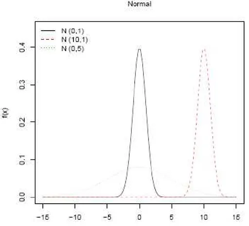
The normal distribution is useful in hydrology for describing well-behaved phenomena such as average annual stream flow, or average annual pollutant loadings. The central limit theorem demonstrated that if a random variable X in the sum of n independent and identically distributed random variables with a finite variance, then with increasing n the distribution of X becomes normal regardless of the distribution of the original random variables.

The pdf for a normal random variable X is

              − − = 2 2 ₂ 1 exp 2 1 ) ( x x x x fx x

σ

µ

πσ

X is unbounded both above and below, with mean µx and variance σx2. The normal distribution’s skew coefficient is zero because the distribution is symmetric. The product-moment coefficient of kurtosis, E[(X- µx)4]/ σ4, equals 3.

The two moments of the normal distribution, µx and σx2 are its natural parameters. They are generally estimates by the sample mean and variance in Eq. (2.1.4) and (2.1.5); these are the maximum likelihood estimates if (n-1) is replaced by n in the denominator of the sample variance. The cdf of the normal distribution is not available in closed form. Selected points zp for the standard normal distribution

with zero mean and unit variance are given in Table 2.1-1; because the normal distribution is symmetric, zp=-z1-p.

p 0.5 0.6 0.75 0.8 0.9 0.95 0.975 0.99 0.998 0.999

zp 0.000 0.253 0.675 0.842 1.282 1.645 1.960 2.326 2.878 3.090

Table 3.2-1 Quantiles of the Standard Normal Distribution

Figure 3.2.1-1 Effect of parameters on the Normal pdf, we consider (1) μ = 0, σ = 1; (2) μ = 10, σ = 1; (3) μ = 0, σ = 5.

3.2.2

The Lognormal Distribution

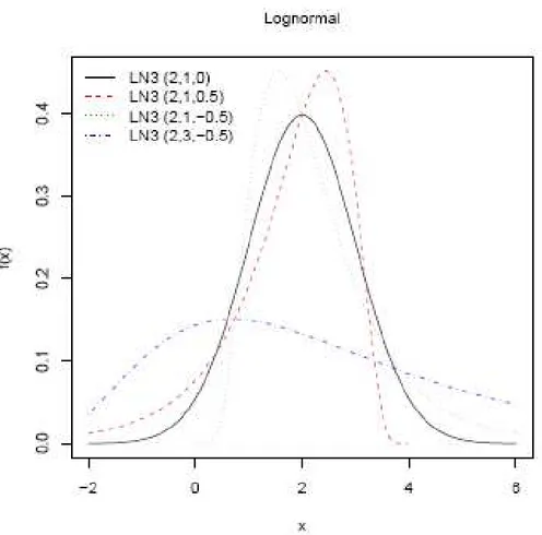
Many hydrologic processes are positively skewed and are not normally distributed. However, in many case for strictly positive random variables X>0, their logarithm

Y = ln (X)

is described by a normal distribution. This is particularly true if the hydrologic sample results from some multiplicative processes, such as dilution.

Inverting the equation above:

X = exp (Y) If X has a lognormal distribution, the cdf for X is

      ₋ Φ =       ₋ ≤ − = ≤ = ≤ = Y Y Y y x y x y Y P x Y P x X P x Fx

σ

µ

σ

µ

σ

µ

) ln( ) ln( )] ln( [ ) ( ) (

where Φ is the cdf of the standard normal distribution.

As a function of the coefficient of variation CVx, the skew coefficient is

γx = 3CVx + CV3

x

As the coefficient of variation and skewness go to zero, the lognormal distribution approaches a normal distribution.

The sample mean and variance of the observed (yi) obtained by using Eq. (2.1.4) and (2.1.5) are the maximum likelihood estimators of the lognormal distribution’s parameters if (n-1) is replaced by n in the denominator of S3y.

Figure 3.2.2-1 2 Effect of parameters on the Normal pdf, we consider (1) ξ = 2, α = 1, k = 0; (2) ξ = 2, α = 1, k = 0.5; (3) ξ = 2, α = 1, k = − 0.5; (4) ξ = 2, α = 3, k =− 0.5.

3.2.3

The Gumbel Distribution

Many random variables in hydrology correspond to the maximum of several similar processes, such as the maximum rainfall or flood discharge in a year. The physical origin of such random variables suggest that their distribution is likely to be one of several extreme value (EV) distributions described by Gumbel. The cdf of the largest of n independent variates with common cdf F(x) is simply F(x)n. For large n and many choices for F(x), F(x)n converges to one of three extreme value distributions, called type I,II and III. Unfortunately, for many hydrologic variables this convergence is too slow for this argument alone to justify adoption of an extreme value distribution as a model of annual maxima and minima.

Let M1, …, Mn be a set of daily rainfall data, and let the random variable

X=max(Mi) be the maximum for he year. If the Mi are independent and identically

distributed random variables unbounded above, with an exponential like upper tail, then for large n the variate X has an extreme value type Gumbel distribution. For example the annual maximum 24-h rainfall depth are often described by a Gumbel distribution.

The Gumbel distribution has the cdf, mean and variance described in Appendix, the Gumbel pdf is α ξ α ξ

α

− − −

=

x e x

e

e

x

f

(

)

1

where ξ is the location parameter and α is the scale parameter.

The case where ξ =0 and α =1 is called the standard Gumbel distribution. The equation for the standard Gumbel distribution (minimum) reduces to

x e x

e

e

x

f

(

)

=

−

The Gumbel distribution’s density function is very similar to that of the lognormal distribution with γ=1,13. Changing ξ and α moves the centre of the Gumbel pdf and

changes its width, but does not change the shape of the distribution. The Gumbel distribution is asymptotically equivalent to the exponential distribution with cdf :

            − − − =

α

ξ

x x Fx( ) exp exp . (3.2.3-5)

The following is the plot of the Gumbel cumulative distribution function for the maximum case.

While the following is the plot of the Gumbel percent point function for the minimum case.

The cdf is easily inverted to obtain

[

ln( )

]

ln p

x_p =ξ−α − (3.2.3-1)

2 2 ˆ 443 , 1 ) 2 ln( ˆ ˆ

λ

λ

α

= = (3.2.3-2)

If the sample variance s2 was employed, one obtains

s s 7797 , 0 6 ˆ = = π α (3.2.3-3)

The corresponding estimator of ξ in either case is

α

ξˆ= x−0,5772ˆ (3.2.3-4)

The form of the Gumbel probability paper is based on a linearization of the cdf. From Equation (3.2.3-5), the Gumbel probability paper resulting from this linearized cdf function is shown next.

L-moments estimators for the Gumbel distribution are generally so good or better than method-of-moment estimators when the observations are actually drawn from case. However, L-moments estimators have been shown to be robust , providing more accurate quantile estimators than product moment and maximum-likelihood estimators when observations are drown from a range of reasonable distributions for flood flows.

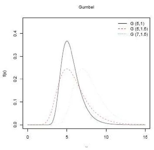
• The shape of the Gumbel distribution is skewed to the left. The Gumbel pdf (Gumbel probability density function) has no shape parameter. This means that the Gumbel pdf has only one shape, which does not change.

• The Gumbel pdf has location parameter µ, which is equal to the mode, but it differs from median and mean. This is because the Gumbel distribution is not symmetrical about its ξ.

• As ξ decreases, the pdf is shifted to the left.

• As ξ increases, the pdf is shifted to the right.

• As σ increases, the pdf spreads out and becomes shallower.

• As σ decreases, the pdf becomes taller and narrower.

• _{For T} =±∞_{, pdf = 0. For T = ξ, the pdf reaches its maximum point }

     e σ 1

Figure 3.2.3-1 Effect of parameters on Gumbel pdf, we consider (1)ξ = 5, α = 1; (2) ξ = 5, α = 1.5; (3) ξ = 7, α = 1.5

3.2.4

The Generalized Gumbel Distribution (GEV)

The Generalized Extreme Value (GEV) Distribution is a general mathematical formulation which incorporates Gumbel’s type I,II and III extreme value distributions for maxima. The GEV distribution’s cdf can be written

            − − − = k x k x Fx / 1 ) ( 1 exp ) (

α

ξ

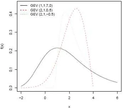
The Gumbel distribution is obtained when k=0. For |k|<0,3 the general shape of the GEV distribution is similar to the Gumbel distribution, though the right-hand tail is thicker for k<0 and thinner for k>0.

Here ξ is a local parameter, α is a scale parameter and k is the important shape parameter. For k>0 the distribution has a finite upper bound at ξ+α/k and corresponds to the EV type III distribution for maxima that are bounded above; for k<0, the distribution has a thicker right-hand tail and correspond to the EV type II distribution for maxima from thick-tailed distributions like the generalized Pareto distribution with k<0.

The moments of the GEV distribution can be expressed in terms of the gamma function Γ(·), or k>-1/3 the mean and variance are given in Appendix.

Figure 3.2.4-1 Effect of parameters on GEV pdf, we consider (1) ξ = 1, α = 1.7, k = 0; (2) ξ = 2, α = 1, k = 0.5; (3) ξ = 2, α = 1, k = −0.5.

3.2.5

The Weibull Distribution

The Weibull Distribution is developed as the extreme value type III distribution for minima bounded below by zero.

If Wi are the minimum stream flows in different days of the year, then the annual minimum is the smallest of the Wi, each of which is bounded below by zero. In this case the random variable X=min(Wi) may be well described by the EV type III distribution for minima, the Weibull distribution’s cdf, mean and variance are included in Appendix. The skewness coefficient is the negative of that of GEV distribution, the second L moment is

λ2 = α(1-2-1/k) Γ(1+1/k)

There are important relationship between the Weibull, Gumbel and GEV distributions. If X has a Weibull distribution, then Y= -ln(X) has a Gumbel distribution. This allows parameter estimation procedures and goodness-on-fit tests available for the Gumbel distribution to be used for the Weibull, thus if ln(X) has mean λ1,(lnX) and L-moment λ2,(lnX), X has Weibull parameters

k=ln(2)/ λ2,(lnX) and α = exp(λ1,(lnX) + 0,5772/k)

3.3

P

LOTTING

P

OSITIONS AND

P

ROBABILITY

P

LOTS

Probabilistic plots are extremely useful visually revealing the character of data sets. The graphical evaluation of the adequacy of a fitted distribution is generally performed by plotting the observations so that they would fall approximately on a straight line if a postulated distribution were the true distribution from which the observations were drown. This can be done with the use of special commercially available probability papers for some distributions, or with the more general techniques presented here, on which such special papers are based.

Let {Xi} denote the observed values and X(i) the ith largest value in a sample, so

that X(n)≤X(n-1)≤ … ≤X(i). The random variable Ui defined as

correspond to the the exceedance probability associated with the ith largest observation. If the original observations were independent, in repeated sampling the Ui have beta distribution with mean

E[Ui] = i/(n+1) (2.1.3.2) and variance ) 2 ( ) 1 ( ) 1 ( ) ( ₂ + + + − = n n i n i Ui Var (2.1.3.3)

Knowing the distribution of the exceedance probability Ui, one can develop

estimators qi of their values which can be used to plot each X(i ) against a probability

scale.

Let G(x) be a proposed cdf for the events. A visual comparison of the data and a fitted distribution is provided by a plot of the ith largest observed event X(i) versus an

estimate of what its true value should be. If G(x) is the distribution of X, the value of X(i) = G-1(1- Ui) should be nearly G-1(1-qi), where the probability plotting position qi

is our estimate of Ui. Thus the points [G-1(1-qi), X(i )] when plotted would, apart from

sampling fluctuation, lie on a straight line through the origin.

The exceedance probability of the ith largest event is often estimated using the Weibull plotting position:

1 + = n i qi (2.1.3.4)

corresponding to the mean of Ui.

3.3.1

Choice of Plotting Position

Hazen originally developed probability paper and imagined the probability scale divided into n equal intervals with midpoints qi = (i-0,5)/n, i=1, …, n; these served as his plotting positions. Gumbel rejected this formula in part because it assigned a return period of 2n years to the largest observation, Gumbel promoted Eq. (2.1.3.4).

Cunanne argued that plotting positions qi should be assigned so that on average X(i ) would equal G-1(1-qi), that is qi would capture the mean of X(i ) so that

E[X(i )] ≈ G-1(1-qi)

Such plotting position would be almost quantile-unbiased. The Weibull plotting position i/(n+1) equal the average exceedance probability of the ranked observation X(i), and hence are probability-unbiased plotting positions. The two criteria are

different because of the nonlinear relationship between X(i) and Ui.

Different plotting positions attempt to achieve almost quantile-unbiasedness for different distributions; many can be written

a n a i qi 2 1− + − =

which is symmetric so that qi = 1-qn+1-i. Cunanne recommended a=0,40 for

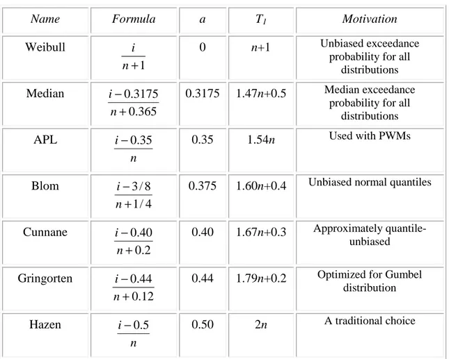
obtaining nearly quantile-unbiased plotting positions for a range of distributions. Other alternatives are Blom’s plottin position (a=3/8) which gives nearly unbiased quantiles for the normal distribution, and the Gringorten position (a=0,44) which yields optimized plotting positions for the largest observations from a Gumbel distribution. These are summarized in Table 2.1.-2, which also reports the return period T1 = 1/q1 , assigned to the largest observation.

The difference between the Hazen formula, Cunanne’s recommendation and the Weibull formula is modest for i of 1 of 3 or more. However, differences can be appreciable for i=1, corresponding to the largest observation. It is important to remember that the actual exceedance probability associated with the largest observation is a random variable with mean 1/(n+1) and a standard deviation of nearly 1/(n+1), see Eq. (2.1.3.2) and (2.1.3.3). Thus all plotting positions give crude estimates of the unknown exceedance probabilities associated with the largest (and smallest) event.

Table 3.3-1 Alternative Plotting Positions

Name Formula a T1 Motivation

Weibull

1

+

n

i 0 n+1 Unbiased exceedance probability for all

distributions Median 365 . 0 3175 . 0 + − n i 0.3175 1.47n+0.5 Median exceedance

probability for all distributions APL n i−0.35 0.35 1.54n Used with PWMs Blom 4 / 1 8 / 3 + − n

i 0.375 1.60n+0.4 Unbiased normal quantiles

Cunnane 2 . 0 40 . 0 + − n i 0.40 1.67n+0.3 Approximately quantile-unbiased Gringorten 12 . 0 44 . 0 + − n

i 0.44 1.79n+0.2 Optimized for Gumbel

distribution

Hazen

n

4

PROBABLE MAXIMUM

PRECIPITATION

For design of high-hazard structures as spillways on large dams it is necessary to use precipitation values with very low risk of exceedance. Ideally a hydrologist would like to choose design storms for which there is no risk of exceedance. A theoretical problem that has plagued the search for such a storm is determining whether there is indeed an upper limit of rainfall amount.

The existence of an upper limit on rainfall is both mathematically and physically realistic (Gilman,1964). The spatial and temporal context of the upper bond on rainfall amount is incorporated into the definition of probable maximum precipitation (PMP), which is defined as “theoretically the greatest depth of precipitation for a given duration that is physically possible over a given size storm area at a particular geographical location at a certain time of year.” A more troublesome problem than ascertaining whether an upper bond exists is determining what it is.

Observed rainfall totals worldwide provide a broad indication of maximum possible rainfall totals at a point as function of duration.

The estimation of probable maximum precipitation was developed and has evolved in the United States as a hydrometeorological procedure. Three meteorological components determine maximum probable precipitation:

1. amount of precipitable water 2. rate of convergence

3. vertical motion

Meteorological models representing all three components have been developed, but it has proved quite difficult to specify maximum rates of areal convergence and vertical motions for the models. In the standard approach to estimating PMP observed storm totals for extreme storms are used as indicators of the maximum values of convergence and vertical motions. The two major components of the

standard approach to the PMP computation are moisture maximization and storm transposition. In the first step of moisture maximization, the goal is to increase storm rainfall amounts to reflect the maximum possible moisture availability. In the storm transposition step, it is determined whether a given storm, which occurred in a broad region around the basin of interest, can be transposed to represent rainfall over the basin.

The principal data required for standard PMP computations are: 1. a catalogue for extreme storms

2. surface dew-point temperature observations

The storm catalogue for Austria and Italy contains storm date, location and depth. Additional meteorological information, including surface and upper-air maps, is typically used subjectively in determining storm transposition regions and for other quality-control purpose. Surface dew-point is used as a moisture index for moisture maximization . Precipitable water can be computed from surface dew-point values under the assumption that saturation levels extend to the ground.

Storm transposition is based on the assumption that for a given storm meteorologically homogeneous regions exist over which the storm is equally likely to occur. The transposition procedure involves meteorological analysis of the strom to be transposed, determination of transposition limits, and application of adjustments for changes in storm location. Meteorological analysis provides a characterization of key aspects of storm type. Transposition limits are determined from a long series of daily weather charts by identifying the boundary of the region over which meteorologically similar storm type have occurred. Adjustments account for differences in moisture maxima for the storm location and transposition sites. Adjustments are sometimes also made for topographic effects, although objective procedures for determining orographic adjustments are not widely accepted.

Having obtained a series of storms, PMP is determined by envelopment. Envelopment entails selection of the storm which has the largest maximised storm rainfall for a given time interval.

The envelopment process is used because a single historical storm is generally not the critical event the entire range of time scales required.

5

PROBABILISTIC ENVELOPE

CURVES FOR EXTREME FLOODS

This chapter wants to introduce the method developed by Castellarin et.al, 2005 for the estimation of extreme floods by envelope curves and for the assumption of their connected probability. This method has been rearranged in order to make it applicable to extreme rainfall events, both to annual maximum series and peaks-over-threshold series . The following methodology will be then applied not to floods as explained, but to extreme rainfall events in different ways for Austrian and Italian catchments, as discussed in Chapter 7.

Next paragraphs propose the original probabilistic interpretation of envelope curves and the formulation of an empirical estimator of the recurrence interval T associated with a REC.

5.1

D

EFINITION OF

R

EGIONAL

E

NVELOPE

C

URVES

A regional envelope curve (REC) summarizes the current bound on our experience of extreme floods in a region. Although RECs are available for many regions of the world, their traditional deterministic interpretation limits the use of the curves for design purposes, as magnitude, but not frequency of extreme flood events, can be quantified. A probabilistic interpretation of a REC is introduced via an estimate of its exceedance probability.

The bound on our experience of extreme floods gained up to the present through systematic observation of flood discharges in a region is defined in terms of the largest floods observed at all gauging stations in a region. Herein, the largest flood is termed the record flood, and gauging stations are referred to as sites. An example of a REC is illustrated in Figure 5-1 which plots, for each site, the normalized record flood, defined as the logarithm of the ratio of the record flood to its basin area, versus

the logarithm of the basin area. The REC is the line drawn on Figure 5-1 which provides an upper bound on all the normalized record floods at present.

Figure 5-3.3.1-1 Q in feet3/s (1foot=0.3048 m) and A in miles2 (1 mile=1.609km) [Jarvis, 1925]: elements of experience (pluses) and element of experience (circle) defining the intercept of the envelope curve (shaded line).

The idea of bounding our flood experience dates back to Jarvis [1925], who presented a REC based on record floods at 888 sites in the conterminous United States. Roughly 50 years later, Crippen and Bue [1977] and Crippen [1982] updated the study by Jarvis [1925] by creating 17 different RECs, each for a different hydrologic region within the United States, based on a total of 883 sites. Matalas [1997] and Vogel et al. [2001] document that the

RECs identified by Crippen and Bue [1977] and Crippen [1982] still bound our flood experience gained from 1977– 1994 at 740 of the 883 sites compiled by Crippen and Bue. Enzel et al. [1993] examine the REC bounding the historical flood experience for the Colorado river basin and show that the same REC also bounds the paleoflood discharge estimates available for the basin.

The development of RECs is not confined to the United States; they have been developed for Italy [Marchetti, 1955], western Greece [Mimikou, 1984], Japan

[Kadoya, 1992], and elsewhere. RECs have been used to compare record flood experience in the United States, China, and the world by Costa [1987] and, more recently, by Herschy [2002].

The REC provides an effective summary of our regional flood experience. The pioneering work of Hazen [1914], who formalized flood frequency analysis, a formalism still in use, and who was among the first to suggest a method for improving information at a site through the transfer of information from other sites (i.e., substitution of space for time), has tempered the use of a flood magnitude as a design flood without an accompanying probability statement. Our objective is to provide a probabilistic interpretation of the REC. In the almost 80 years since Jarvis [1925] introduced the envelope curve, a probabilistic interpretation of a REC has never been seriously addressed.

RECs have continued to be constructed and viewed mainly as summary accounts of record floods, rather than as meaningful tools for the design of measures to protect against ‘‘catastrophic’’ floods. It has been suggested that there is no obvious way to assign a probabilistic statement to a REC [see, e.g., Crippen and Bue, 1977; Crippen, 1982; Vogel et al., 2001]. Water Science and Technology Board, Commission on Geosciences, Environment and Resources [1999] argued that the determination of the exceedance probability of a REC is difficult due to the impact of intersite correlation. As a consequence, RECs are assumed to have little utility beyond the suggestion of the U.S. Interagency Advisory Committee on Water Data [1986] that they are useful for ‘‘displaying and summarizing data on the actual occurrence of extreme floods.’’ A probabilistic interpretation of the REC offers opportunities for several engineering applications which seek to exploit regional flood information to augment the effective record length associated with design flood estimates.

A potential advantage of assigning a probabilistic statement to a REC is that this approach avoids the need to extrapolate an assumed at-site flood frequency distribution hen estimating a design event.

This work would provide a probabilistic interpretation of the REC, to approximate its exceedance probability, and to quantify the effect of intersite correlation on estimates of the exceedance probability and extend their utilisation from floods to rainfall events.

5.2

A

P

ROBABILISTIC

I

NTERPRETATION OF

E

NVELOPE

C

URVES

It is common practice to construct a REC, as in Figure 5-1, which plots the logarithm of the ratio of the record flood to the drainage area, ln(Q/A) versus ln(A). Jarvis [1925] suggested modeling the REC for the United States using,

) ln( ln a b A A Q + = (5.1-1)

with a = 9.37 (or a = 4.07 if log is used in (5.1-1) instead of ln) and b = -0.50, where Q and A are in cubic feet per second and square miles, respectively. Together with Jarvis [1925], other empirical studies showed that b is negative and greater than 2/3 for various portions of the world [Linsley et al., 1949; Marchetti, 1955; Crippen and Bue, 1977; Matalas, 1997; Herschy, 2002].

Assuming a fixed value of b, the intercept a in (5.1.1) may be estimated by forcing the REC to bound all record floods to the present, say up to the year n. Let Xj i denote

the annual maximum flood in year i = 1, 2, . . .,n at site j = 1, 2, . . .M, where M is the number of sites in the region.

Let Xj (i) denote the flood flow of rank (i) at site j, where ranking is from smallest

(1) to largest (n). The REC’s intercept up to the year n can then be expressed as

        −         = = ln ln( ) max ) ( ,..., 1 ) ( j j n j M j n A b A X a

where Aj is the area of site j = 1, 2, . . .M.

5.3

D

ESCRIPTION OF THE

M

ETHOD

The probabilistic regional envelope curves (PRECs) developed by Castellarin et al, 2005 presented a probabilistic interpretation of the envelope curve presented in equation (5.1-1). The proposed probabilistic regional envelope curves (PRECs) are based upon two fundamental assumptions:

1. the group of river basins (i.e., geographical region or pooling group of sites is homogeneous in the sense of the index flood hypothesis

2. the relationship between the index flood µx (e.g. mean annual flood) and A is of the form, 1 + = b CA x

µ

where b and C are constants and b is the same as in equation (5.1-1).

Under these assumptions has been developed an empirical estimator of the exceedance probability p of the expected PREC. The expected PREC is the envelope curve that, on average, is expected to bound the flooding experience for a region of given characteristics (i.e., M sites with record length n and mean intersite correlation

ρ). The expected PREC is identified through a series of Monte Carlo simulations experiments by generating a number of synthetic cross-correlated regions consisting of M concurrent sequences of annual maximum flood with record length n. It is proposed an estimator of p of the expected PREC that is a function of the effective number of sites, MEC ≤ M (i.e., number of independent flood series with an

equivalent information content).

The recurrence interval of the expected PREC can then be computed as the inverse of p. Assigning an exceedance probability, or equivalently a recurrence interval, to a PREC makes it a practical tool for estimating a design event at gauged and ungauged river basins.

We present an algorithm for the application of the empirical estimator of p to historical annual maximum series of unequal length.

5.3.1

Estimating the Effective Number of Sites

The problem of estimating the exceedance probability p of the expected PREC reduces to estimating the exceedance probability of the largest value in a regional sample of standardized annual maximum peak flows.