ALEA
Tech Reports
Testing the Profitability of Simple Technical
Trading Rules: A Bootstrap Analysis of the
Italian Stock Market
Marco Bee, Amedeo Gazzini
Tech Report Nr. 18
Marzo 2004
Alea - Centro di ricerca sui rischi finanziari
Dipartimento di informatica e studi aziendali
Università di Trento - Via Inama 5 - 38100 - Trento
http://www.aleaweb.org
Testing the Profitability of Simple Technical Trading Rules:
A Bootstrap Analysis of the Italian Stock Market
Marco Bee∗, Amedeo Gazzini∗∗
∗ Intesa Bank,
Risk Management, Piazza Ferrari 10, I-20121 Milano - Italy
∗∗ Dresdner Kleinwort Wasserstein,
Capital Markets Principal Trading, Theodor-Heuss-Allee 44,
D-61092 Frankfurt am Main - Germany,
ABSTRACT
The aim of this paper consists in testing the profitability of simple technical trading rules in the Italian stock market. By means of a recently developed bootstrap methodology we assess whether technical rules based on moving averages are capable of producing excess returns with respect to the Buy-and-Hold strategy. We find that in most cases the rules are profitable and the excess return is statistically significant. However, the well-known problem of data-snooping, which seems to be confirmed by our analysis, requires some caution in the application of these methods.
Key words: Technical Analysis, Data-Snooping, Resampling Methods, Sharpe Ratio.
1 Introduction
Technical analysis can de defined as a set of heterogeneous tools whose purpose consists in forecasting future prices on the basis of historical prices and market statistics. The development of these methods can be traced back to the late 1800’s, but, until recent years, financial theory has always been biased against technical analysis. The literature generated by the debate confronting technical analysts and academics is huge; although it is impossible to enter into details here (see Beber 1999 for a review), it is worth giving an up-to-date summary. Before we start dealing with technicalities, this will indeed help clarifying the aim of this paper.
The dispute has mainly to do with the following question: is the market efficient? If the answer is positive, current prices fully incorporate all available information; in this case, it is not difficult to show that the expected value of the returns of any strategy based on time-t information is equal to zero, and the data generating process (DGP) of the returns is the random walk; in this case, technical analysis would be useless. On the other hand, if the answer is negative, current prices do not incorporate all available information, and therefore they are different from their equilibrium level, so that using historical information to determine the equilibrium price can be profitable, as it is different from the current price.
Early tests of market efficiency were mostly indirect, i.e., they tested the random walk hypothesis (see Campbell et al. 1997, chap. 2). Direct tests, which investigate whether specific trading rules are profitable, have been developed more recently, and were mostly spurred by practitioners’ interests: not surprisingly, the role of trading rules became quickly the main object of analysis. In the latter category, bootstrap methods have been extensively used (LeBaron 1991, Brock et al. 1992, Kim 1994, Karolyi and Kho 1994, Le Baron 1996); however, their application to a time series setup, where data are not independent, is not as straightforward as the classical bootstrap with indepen-dent and iindepen-dentically distributed (iid) data, so that these experiments produced mixed evidence (see Maddala and Li 1996 for a critical review). Moreover, the procedure is too complicated to give traders quick indications useful for taking positions in the market. A major improvement has been achieved by Sullivan et al. (1999); their methodology, which allows a fully non-parametric implementation of the bootstrap, will be used, with some modifications, in this paper.
weak-ened, as witnessed by the growing number of papers published in academic journals about the relationship between financial and econometric theory on one hand and meth-ods used by practitioners on the other hand (Lo et al. 2000, Osler 2003). The efficient market hypothesis has indeed been questioned by several empirical studies, and although there is no agreement about the reason (market inefficiency and time-varying equilib-rium returns being the most likely ones), the belief that future returns are predictable on the basis of past returns is now, at least, an issue which deserves investigation. More-over, Kavajecz and Odders-White (2003) recently introduced a new approach which tries to explain the predictability of returns by means of limited order book liquidity, so that technical analysis would be consistent with market efficiency.
The aim of this work consists in testing whether the most common trading rules, i.e. moving average-based rules, are profitable in the Italian stock market and providing directions about their practical application. Overall, we find that the trading rules are profitable; statistical significance is higher for rules based on short moving averages, for which the number of trades is larger and consequently the transaction costs are higher. Further analysis shows that profitability is more questionable when we explicitly take into account transaction fees.
The rest of the paper is organized as follows. Section 2 describes the data and the technical trading rules used for the test; section 3 provides details of the testing methodology; section 4 shows the results of the empirical analysis; section 5 concludes.
2 Data and technical rules description
2.1. Data description
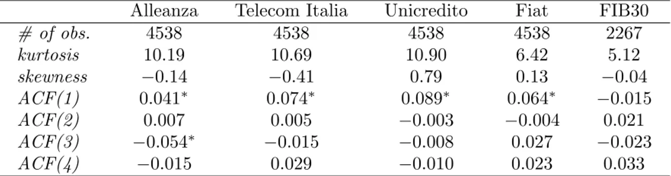
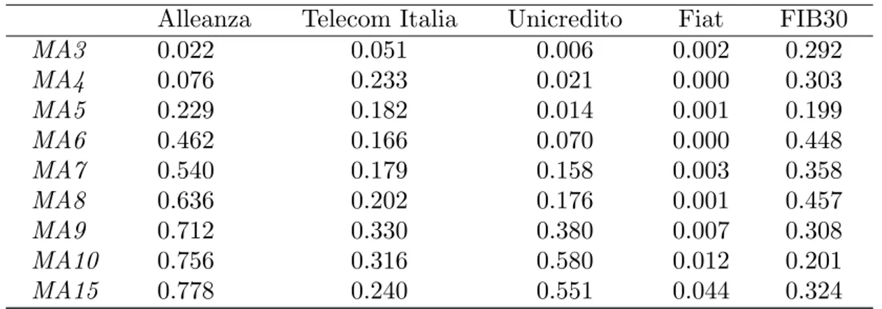
For our test we will use daily data of four of the most liquid Italian stocks: Alleanza, Telecom Italia, Unicredito and Fiat. The sample period is August 15, 1985 to January 6, 2003. We will also perform the calculations using data of the FIB30 index, i.e. the future on the MIB30 index; in this case the sample period is November 28, 1994 to August 5, 2003. The main reason for the inclusion in the analysis of the latter data is that dividends, which are ignored in the computations concerning individual stocks, are of no concern with futures data. All the data, here and in the following, were downloaded from Bloomberg. Standard descriptive statistics are shown in table 1; figures 1 and 3a show the histograms of daily returns, whereas figures 2 and 3b show the levels.
Table 1. Descriptive statistics. Numbers marked with∗ are significant at the 5% level.
Alleanza Telecom Italia Unicredito Fiat FIB30
# of obs. 4538 4538 4538 4538 2267 kurtosis 10.19 10.69 10.90 6.42 5.12 skewness −0.14 −0.41 0.79 0.13 −0.04 ACF(1) 0.041∗ 0.074∗ 0.089∗ 0.064∗ −0.015 ACF(2) 0.007 0.005 −0.003 −0.004 0.021 ACF(3) −0.054∗ −0.015 −0.008 0.027 −0.023 ACF(4) −0.015 0.029 −0.010 0.023 0.033
Unsurprisingly, from the table and the figures it turns out that the data show some serial correlation and are leptokurtic.
Finally, it is worth noting that dividends are ignored; this omission could lead to a few mistakes when computing the returns for the individual stocks, as the price of a stock drops after the dividend payment. However, usually dividends are rather small, so that this way of proceeding should not introduce any major bias.
2.2. Technical trading rules
An extremely large number of trading rules have been developed over the years (see Appendix A in Sullivan et al. 1999 for a review). As this paper also aims at taking into account what traders do in practical applications, we will focus on rules based on moving averages, which are indeed widely used and can be tested without being computationally cumbersome.
At time t, the moving average of length R is given by
M A(R)t = 1 R
R−1! i=0
Pt−i, t = R, R + 1, . . . , T.
The basic idea underlying the use of moving averages as trading signals is the following. Suppose that
Pt−1 < M A(R)t−1 and Pt ≥ MA
(R)
t ; (1)
in this case we assume that an upward trend has initiated, and therefore we take a long position. Similarly, if
we are confident that we are entering a downward trend, and we take a short position. Numerous modifications of (1) and (2) have been developed; we mention here the in-troduction of a band b > 0 around the moving average so that a long position is taken
when Pt ≥ MA(R)t + b · MA(R)t and closed when Ps < M A(R)s (s > t); similarly, a short
position is opened when Pt < M A(R)t − b · MA(R)t and closed when Ps ≥ MA(R)s (s > t);
the introduction of the band should help avoiding the so called “false signals”. According to these indications, a signal function can be defined as follows:
St = 1 if Pt ≥ MA(R)t + b · MA (R) t 0 if MA(R) t − b · MA (R) t ≤ Pt < M A(R)t + b · MA (R) t −1 if Pt < M A(R)t − b · MA (R) t , t = R, . . . , T . (3)
Notice that, if b = 0, St can only take value 1 or −1, i.e. the trader is always in the
market.
3 Testing Methodology
The classical way of testing the performance of trading rules consists in applying the rules to a long time series of returns of the traded security and defining a ranking based on the excess returns over a benchmark model, usually the Buy-and-Hold (B/H) strategy.
When tackling this problem, we are immediately confronted with a difficulty: trad-ing rules lack theoretical foundations. In principle, this implies that any mechanical rule could work and the set of rules to consider is infinite. This issue was first identified by Jensen and Bennington (1970, pag. 470): “given enough computer time, we are sure that we can find a mechanical trading rule which “works” on a table of random
numbers - provided of course that we are allowed to test the rule on the same table of
numbers which we used to discover the rule”. It is strictly related to what is currently known under the name of data-snooping (Brock et al. 1992, LeBaron 1996, Sullivan et
al. 1999). In essence, data-snooping means that the “best” trading rule is chosen on the
basis of the returns obtained from the application to an observed data series (that is, a single realization of the data generating process), and its superior performance could only hold for this realization.
Historically, in order to get around these difficulties, researchers have focused on two methodologies. The simplest solution consists of splitting the observed series in two periods; the first one (in-sample) is used to find the best trading rule, whereas the
second one (out-of-sample) checks whether the ranking of the rules found in the first period is preserved when the rules are applied to data from a different period.
The second methodology is based on the non-parametric bootstrap introduced by Efron (1979); in the context of testing the efficiency of technical trading rules, different variants were employed by Brock et al. (1992), LeBaron (1996) and Sullivan et al. (1999). The non-parametric bootstrap with iid observations is based on drawing with re-placement B samples from the data at hand, where B is a “large” number; more
for-mally, this means sampling from the empirical distribution function FN, which puts
probability 1/N on each observation; it can be shown that the empirical distribution obtained in this way converges to the true distribution. However, it is quite clear that the observations at hand are likely to be neither independent (because of serial corre-lation) nor identically distributed (because of time-varying volatility), so that the basic bootstrap might not be adequate.
To make things worse, when working with financial data a major difficulty arises: it is not appropriate to bootstrap directly the time series of prices. In fact, if we follow this way (see Maddala and Li 1996, pag. 466, for details), we do not perform any model specification testing before bootstrapping, so that we run the risk of bootstrapping the wrong model.
Over the years, this problem has been tackled in two ways. The first solution consists of fitting a model to the time series of prices, bootstrapping the residuals and generating bootstrap samples using the estimated parameters; this approach was implemented by Brock et al. 1992 on American stock indices, and then by Hudson et
al. (1996) on UK data and by Isakov and Hollistein (1999) on Swiss data. However, all
of them found that specifications like random walk, AR(1) and GARCH do not seem to work well, so that more complicated formulations would be called for.
The second solution (employed, for example, by LeBaron 1996) resamples the orig-inal return series and then reconstructs the price series according to a prespecified stochastic model for price evolution. Again, this is likely to be severely influenced by the choice of the DGP; if the assumed DGP is different from the true DGP, the method will produce wrong results.
As can be seen from these remarks, using the bootstrap with financial data is rather dangerous. Maddala and Li (1996) thoroughly summarize the results of early applica-tions: they point out that in many cases bootstrap methods were not applied correctly
and are thus likely to have produced spurious results. They also notice that, even though the final goal consists in checking profitability, model identification is crucial in order to get meaningful results. It follows that the method is much less appealing in this context than in the classical iid setup, where no distributional assumption is re-quired: the need for a specification of a parametric model for price evolution constitutes indeed a significant drawback. Moreover, a procedure which requires traders to carry out model identification and estimation and then implement bootstrap to finally obtain the desired result is clearly too laborious to be useful in practical applications.
A new approach has recently been developed by Sullivan et al. (1999) on the basis
of results obtained by White (2000) (1): it consists of resampling directly the returns
from the trading rules; the advantage of this solution is that model identification is
completely avoided. From a technical point of view, it has been shown by White (2000) that this way of proceeding has all the desirable properties of the standard bootstrap (for an accessible review of the results see appendix B of Sullivan et al. 1999).
To begin with the description of the methodology, let
¯f = n−1
T ! t=R
ft+1
be the “performance statistic”, where R is the length of the longest moving average and
n = T − R + 1 (starting the indexing from R just means that the first R data are only
used to compute the moving average). ft is a v × 1 vector, where v is the number of
trading rules and fit, the i-th element of ft, gives the time-t excess return from the i-th
trading rule:
fit = Sit· log(Pt+1/Pt) − S0t· log(Pt+1/Pt), i = 1, . . . , v; t = R, . . . , T.
Notice that S0t identifies the benchmark model, which in the following is given by the
B/H strategy. Sit is a signal function which takes values in the set {1, 0, −1}: for moving
average-based rules it has already been defined in (3). The values −1, 0 and 1 represent short, neutral and long positions respectively.
The null hypothesis we are interested in is that the technical trading rule’s perfor-mance is no better than the perforperfor-mance of the B/H strategy:
H0 : E(fi) ≤ 0, i = 1, . . . , v. (4)
(1) Careful readers are certainly thinking that (at least) one of these dates is wrong, but both of them are
indeed correct; nevertheless, for this sentence to make sense, we have to admit that White’s results must have been obtained before 2000...
In terms of profitability, we hope to be able reject H0; this would mean that the
differ-ence between the return from the trading rule and the return from the B/H strategy is statistically significant.
Sullivan et al. (1999) implicitly assume that every conceivable trading rule has the same chance of being the best one; according to this starting point, it is clear that the analysis has to test simultaneously all possible rules, because it could be that the most commonly used trading rules, which are typically the ones that historically have shown the best performance, have been considered “best” just because of data-snooping. They point out that these trading rules could have emerged as superior as the result of a “subtle survivorship bias”: historically, investors tried out numerous rules, but after a while they kept using only a small subset of them (the “best” rules). If these ones had emerged in virtue of data-snooping, then the only way of discovering it would consist in confronting them with the neglected rules as well.
This approach has the obvious drawback of being computationally cumbersome, because a huge number of trading rules needs to be considered; in addition, the require-ment of checking all possible rules seems to be very difficult to fulfill as the set of rules is in principle infinite. For these reasons we will introduce some modifications.
In our opinion it is unlikely for a rule to have arisen as a well-performing one only because of data-snooping: typically, these rules have indeed been checked independently by many researchers using different data and/or time horizons, so that we believe they do have some economic content. The bootstrap has a central role here: if a rule is not effective, the bootstrap will certainly allow us to discover it. In summary, we prefer to rely on the hypothesis (that we believe has an high probability of being true) that the most commonly used trading rules are also the “best” ones. Because of the bootstrap check, there is essentially no risk of making incorrect inferences about trading rules: if this assumption is not supported by the data, the bootstrap will reveal it. In this way the results are more easily interpreted and the computational burden is much smaller.
Thus, we apply the bootstrap to the observed values fi,R, fi,R+1, . . . , fi,T of the
returns from each trading rule and obtain B bootstrapped values of ¯fi, denoted by
¯
fi∗(j), where j indexes the B bootstrap samples. Finally, we compute the following
statistics:
¯
Vi =√n ¯fi; ¯
Vi∗ =√n( ¯fi∗− ¯fi).
To take into account the features of time series data, several extensions of the basic bootstrap have been developed (Davison and Hinkley 1997, chap. 8); all of them are based on the concept of block bootstrap. The simplest version of this technique
subdivides the data into k non-overlapping blocks of length l, z1 = (x1, . . . , xl), z2 =
(xl+1, . . . , x2l), . . . , zk = (xkl−l+1, . . . , xkl), where kl = N. Instead of resampling single
observations, each bootstrap replication resamples blocks of consecutive observations. In this way we try to preserve some of the dependence of the original data; in general we observe that the “proportion of dependency” captured by the series so reconstructed is positively related to l; obviously, with l = N the series will have the same dependency of the original series. The choice of the block length has therefore to consider two contrasting requirements: on one hand l should be large in order to preserve as much as possible of the dependency of the original series; on the other hand, one wants to have a large number of distinct bootstrap replications in order to reliably use the the asymptotic theory which underlies the bootstrap, and this would require many short blocks (that is, large k and small l).
Various modifications of the the block bootstrap have been considered; in the fol-lowing we will use the stationary bootstrap introduced by Politis and Romano (1994) and applied in the same context by Sullivan et al. (1999). This approach resamples from non-overlapping blocks of random length L, where L has a geometric distribution of parameter p = 1/l:
P (L = l) = (1− p)l−1p, l = 1, 2, . . . (5)
As shown by Politis and Romano (1994), series obtained by means of this approach are stationary.
It is hardly worth noting that a statistical test for the hypothesis (4) could be easily constructed, by means of standard arguments, under the assumption of normality (see, for example, Brock et al. 1992, pag. 1738); however this assumption is clearly violated here, so that we prefer to rely on the bootstrap approach only.
4 Empirical Results
4.1. Results for the mean return criterion
We first test the behavior of technical rules when the performance measure is the mean annualized return, i.e. the daily return multiplied by 261, the number of working
days in a year; as usual, daily returns are given by rt = log(Pt/Pt−1). Part A of figures 4 to 8 shows the results: the graphs report the mean annualized return for lengths of the moving average from 3 to 100 days. It is clear that using rules based on short moving averages gives larger returns: for the individual stocks the largest returns are obtained with the 3- and 4-days moving averages; only for the FIB30 index the best results are given by the 10-days moving average.
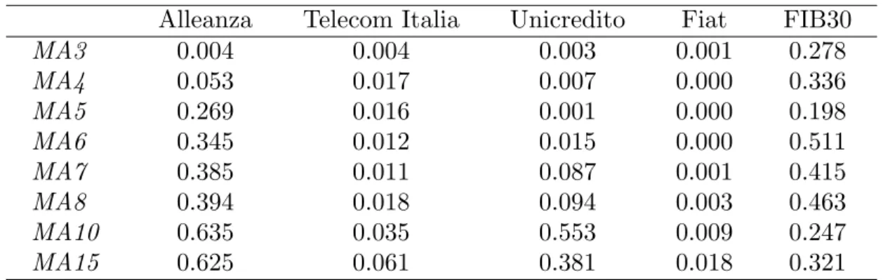
Overall, the returns shown in the figures are surprisingly large; to check whether they are significantly larger than the returns from the B/H strategy, we ran a bootstrap analysis, based on 1000 replications, for the rules which show the largest returns. In the implementation of the stationary bootstrap it is required to specify the parameter p in (5); from the properties of the geometric distribution, the mean block length is equal to 1/p. Given the low serial correlation of our data, we chose p = 0.1, which corresponds to a mean block length of 10. The results are given in table 2. As for p, we performed a small sensitivity analysis by trying out p = 0.01 and p = 0.5; the results obtained are nearly identical to the ones shown in table 2.
Table 2. Bootstrap analysis. The numbers in the table are p-values obtained by comparing V¯i to the
distribution ofV¯∗
i , computed withB=1000replications and lengths of the moving average from 3 to 15 days.
Alleanza Telecom Italia Unicredito Fiat FIB30
MA3 0.004 0.004 0.003 0.001 0.278 MA4 0.053 0.017 0.007 0.000 0.336 MA5 0.269 0.016 0.001 0.000 0.198 MA6 0.345 0.012 0.015 0.000 0.511 MA7 0.385 0.011 0.087 0.001 0.415 MA8 0.394 0.018 0.094 0.003 0.463 MA10 0.635 0.035 0.553 0.009 0.247 MA15 0.625 0.061 0.381 0.018 0.321
Here we observe a marked difference between the behavior of the rules for Telecom Italia, Unicredito and Fiat on one hand and for the FIB30 index on the other hand; in the latter case, excess return is never significant, whereas it is always significant for the three stocks, not only for the single best trading rule but also for the other well-performing strategies. As for Alleanza, empirical evidence is less clear-cut, with the best rule only being significant.
Another question deserves some investigation: is the choice of the trading rule sensitive to changing market conditions? To explore this issue, we follow a strategy
(sometimes called Cumulative Wealth Rule - CWR) which was first introduced by Lukac
et al. (1988). Suppose to have N years of data; in the first step, use the first three years
(in-sample) to find the best strategy, and use it over the fourth year (out-of-sample); in the second step use the second, third and fourth year (in-sample) to find the best strategy, and use it over the fifth year (out-of-sample). Proceed in this way until the final step, where the data of years N − 3, N − 2 and N − 1 are used in-sample and the data of the last year are used out-of-sample. The return from the strategy is finally given by the mean of the returns obtained in the out-of-sample periods.
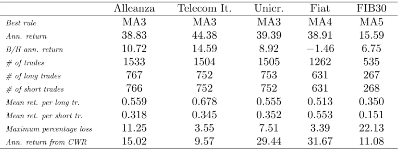
Table 3 provides the result of the CWR as well as some details about the best trading rules; as for the CWR, it outperforms the benchmark, with the exception of Telecom Italia, but its return is smaller than the profit from the best rule; this reflects the important fact that investors could not have known in advance the ex post best-performing strategy. As for the best rules, it is worth noting that, on average, profits from long trades are higher than profits from short trades. Both these findings are actually very similar to the ones obtained by Sullivan et al. (1999, pag. 1667-8).
For practical applications it is important to consider the temporal evolution of the
profit from the rules. It is indeed frequent that, at some time t∗ during the period under
investigation, the trader would lose some money by closing the position in t∗; as it is
quite common to use stop loss rules, it is relevant to quantify the maximum loss from the strategy in the period of application. The results are shown in table 3; it can be seen that using, for example, a 10% stop loss threshold, in two cases out of five (Alleanza and FIB30) we would close the trade before the end of the period.
Table 3. Detailed results for the best rules and returns from the cumulative wealth rule
Alleanza Telecom It. Unicr. Fiat FIB30
Best rule MA3 MA3 MA3 MA4 MA5
Ann. return 38.83 44.38 39.39 38.91 15.59 B/H ann. return 10.72 14.59 8.92 −1.46 6.75
# of trades 1533 1504 1505 1262 535
# of long trades 767 752 753 631 267
# of short trades 766 752 752 631 268 Mean ret. per long tr. 0.559 0.678 0.555 0.513 0.350 Mean ret. per short tr. 0.318 0.345 0.352 0.553 0.151 Maximum percentage loss 11.25 3.55 7.51 3.39 22.13 Ann. return from CWR 15.02 9.57 29.44 31.67 11.08
So far, transaction costs have been ignored; however, in practice, they are obviously important. Part B of figures 4 to 8 shows the number of trades for each strategy, and it can be seen that it is much larger for the rules based on short moving averages, so that it is likely that these rules are not the best ones after the introduction of transaction costs.
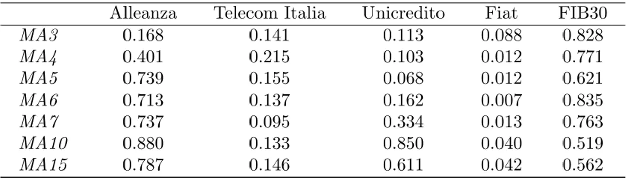
In order to check the impact of transaction costs we ran the same analysis assuming that to each trade is associated a cost c equal to 0.1%, 0.2% and 0.3% (this is supposed to include slippage costs as well). The results are shown in figures 9 to 12. Except for one case (Alleanza), as costs increase, the most profitable rule shifts from the 3-(Telecom Italia, Unicredito) or 4-days (Fiat) moving average to strategies based on longer moving averages. This is particularly apparent for Telecom Italia and for the FIB30 index: with c = 0.3%, the best rules become respectively the 14- and 35-days moving average. The reason is that, with longer moving averages, smaller profits are more than compensated by the decrease in costs determined by the reduced number of trades. However, the next important question is: do the best rules still provide us with a return significantly larger than the B/H strategy? Again, the bootstrap analysis gives us the answer; we show in table 4 the results obtained with c = 0.2%, which seems to be the approximate market level of the transaction costs.
Table 4. Bootstrap analysis. The numbers in the table are p-values obtained by comparing V¯i to the
distribution ofV¯∗
i , computed withB=1000replications and several lengths of the moving average; percentage
cost of a single transaction isc=0.2%.
Alleanza Telecom Italia Unicredito Fiat FIB30
MA3 0.168 0.141 0.113 0.088 0.828 MA4 0.401 0.215 0.103 0.012 0.771 MA5 0.739 0.155 0.068 0.012 0.621 MA6 0.713 0.137 0.162 0.007 0.835 MA7 0.737 0.095 0.334 0.013 0.763 MA10 0.880 0.133 0.850 0.040 0.519 MA15 0.787 0.146 0.611 0.042 0.562
From table 4 it can be seen that the difference between the returns from the trading rules and the B/H strategy is statistically significant only for Fiat (probably because the B/H strategy’s performance is particularly poor in this case).
Finally, we implemented trading rules based on moving averages with a band, as explained in section 2.2. We applied bands b equal to 0.001, 0.005, 0.01, 0.015, 0.02
and 0.03; to save space, results are not shown here but are available upon request. In general, as the band increases, both returns and number of trades get smaller; these rules could therefore be interesting only when transaction costs are high. However, with the costs considered so far, the reduction in the number of trades does not seem to be sufficiently large to guarantee a net profit larger than the one obtained from the moving average rules with no band used before.
4.1. Results for the Sharpe ratio criterion
When evaluating performance, it is of some importance to measure risk-adjusted profits; to this aim we will follow the literature (LeBaron 1996, Sullivan et al. 1999) in computing the Sharpe ratio, which gives the mean excess return per unit risk (see for example Campbell et al. 1997, pag. 188):
SRi =
µi− rf
σfi
, i = 1, . . . , v,
where rf is the risk-free rate. As a proxy of the risk-free interest rate, we use the 3-months Libor rate; due to data availability, here the sample period is January 1, 1989 to January 6, 2003. The null hypothesis of interest is now
H0 : g(E(hi)) ≤ g(E(h0)), i = 1, . . . , v,
where the components of the (3 × 1) vector hi,t+1 are given by
h1i,t+1 = rt+1Sit,
h2i,t+1= (rt+1Sit)2, h3i,t+1= rft+1,
and the function g(·) is defined as follows:
g(E(hi,t+1)) = E(h
1
i,t+1) − E(h3
i,t+1) &
E(h2i,t+1) − (E(h1
i,t+1))2
.
Tables 5 and 6 show respectively the Sharpe ratios computed with the observed data and the bootstrap p-values.
Table 5. Results for the Sharpe ratio criterion. This table reports the Sharpe ratio for the B/H strategy and for trading rules based on several lengths of the moving average.
Alleanza Telecom Italia Unicredito Fiat FIB30
B/H 0.307 0.463 0.224 −0.277 0.264 MA3 1.123 1.090 1.082 0.895 0.524 MA4 0.847 0.757 0.984 1.099 0.525 MA5 0.608 0.831 1.015 1.087 0.679 MA6 0.378 0.828 0.721 0.965 0.291 MA7 0.259 0.843 0.568 0.905 0.435 MA8 0.193 0.802 0.529 0.763 0.340 MA9 0.104 0.683 0.346 0.736 0.472 MA10 0.031 0.715 0.149 0.597 0.608 MA15 0.009 0.740 0.173 0.435 0.433
Table 6. Bootstrap Analysis. The numbers in the table arep-values obtained by applying the bootstrap to the observed values of the Sharpe ratio;B=1000replications.
Alleanza Telecom Italia Unicredito Fiat FIB30
MA3 0.022 0.051 0.006 0.002 0.292 MA4 0.076 0.233 0.021 0.000 0.303 MA5 0.229 0.182 0.014 0.001 0.199 MA6 0.462 0.166 0.070 0.000 0.448 MA7 0.540 0.179 0.158 0.003 0.358 MA8 0.636 0.202 0.176 0.001 0.457 MA9 0.712 0.330 0.380 0.007 0.308 MA10 0.756 0.316 0.580 0.012 0.201 MA15 0.778 0.240 0.551 0.044 0.324
These results essentially confirm (with the partial exception of Telecom Italia) the evi-dence obtained according to the mean return criterion, with the shortest averages being the best ones.
5 Concluding remarks
In this paper we have investigated the profitability of some simple technical trading rules in the Italian stock market. As a general conclusion, the rules seem to give good results: profits from these strategies are significantly larger than profits from the Buy-and-Hold strategy; in particular, short-term moving averages produce the best performances, and the significance of these performances has been confirmed by the bootstrap analysis. The only disturbing aspect is that the evidence is not homogeneous
across assets, as it is highly significant for Telecom Italia, Unicredito and Fiat, significant (but only in the case of the single best-performing rule) for Alleanza and non-significant for the FIB30 index. We do not have an explanation for this phenomenon, which seems to be an example of data-snooping.
Moreover, one should keep in mind that, in practice, it is unreasonable to assume that there are no transaction costs, and the introduction of transaction fees significantly reduces the trading rules’ excess return.
Overall, our findings are in line with the results obtained by other researchers using data from different stock markets. This seems to imply that the features of the most liquid stock markets are similar all over the world and there is thus room for generating significant profits by means of the tools of technical analysis.
References
Beber, A. (1999), “Il Dibattito su Dignit`a ed Efficacia dell’Analisi Tecnica nell’Eco-nomia Finanziaria”, Tech Report nr. 3, Alea, Centro di Ricerca sui Rischi Finanziari, Universit`a di Trento, marzo.
Brock, W., Lakonishok, J. and LeBaron, B. (1992), “Simple Technical Trading Rules and the Stochastic Properties of Stock Returns”, Journal of Finance, 47, 1731-1764.
Campbell, J.Y., Lo, A.W. and MacKinlay, A.C. (1997), The Econometrics of
Financial Markets, Princeton, Princeton University Press.
Davison, A.C., and Hinkley, D.V. (1997), Bootstrap Methods and their Application, Cambridge, Cambridge University Press.
Efron, B. (1979), “Bootstrap Methods: Another Look at the Jackknife”, Annals of
Statistics, 7, 1-26.
Hudson, R.M., Dempsey, M. and Keasey, K. (1996), “A Note on the Weak Form Efficiency of Capital Markets: the Application of Simple Technical Trading Rules to UK Stock Prices - 1935 to 1994”, Journal of Banking and Finance, 20, 1121-1132. Isakov, D. and Hollistein, M. (1999), “Application of Simple Technical Trading Rules to Swiss Stock Prices: Is It Profitable?”, Financial Markets and Portfolio
Man-agement, 13, 9-26.
Jensen, B.C. and Bennington, G.A. (1970), “Random Walk and Technical Theo-ries: Some Additional Evidence”, Journal of Finance, 25, 469-482.
Karolyi, G.A. and Kho, B.C. (1994), “Time-varying Risk Premia and the Returns to Buying Winners and Selling Losers: Caveat Emptor and Venditor”, working paper, Ohio State University.
Kavajecz, K.A. and Odders-White, E. (2003), “Technical Analysis and Liquidity Provision”, Review of Financial Studies, forthcoming.
Kim, B. (1994), “A Study of Risk Premiums in the Foreign Exchange Market”, Ph.D. dissertation, Ohio State University.
LeBaron, B. (1991), “Technical Trading Rules and Regime Shifts in Foreign Ex-change”, working paper, University of Wisconsin.
LeBaron, B. (1996), “Technical Trading Rule Profitability and Foreign Exchange In-tervention”, National Bureau of Economic Research, working paper # 5505.
Analy-sis: Computational Algorithms, Statistical Inference, and Empirical Implementation”,
Journal of Finance, 55, 1705-1765.
Lukac, L.P., Brorsen, B.W. and Irwin, S.H. (1988), “A Test of Futures Market Disequilibrium using Twelve Different Technical Trading Systems”, Applied Economics, 20, 623-639.
Maddala, G.S. and Li, H. (1996), “Bootstrap Based Tests in Financial Models”, in Maddala, G.S. and Rao, C.R. (eds.), Handbook of Statistics, vol. 14, “Statistical Methods in Finance”, Amsterdam, North-Holland.
Osler, C.L. (2003), “Currency Orders and Exchange Rate Dynamics: An Explanation for the Predictive Success of Technical Analysis”, Journal of Finance, forthcoming. Politis, D. and Romano, J. (1994), “The Stationary Bootstrap”, Journal of the
American Statistical Association, 89, 1303-1313.
Ready, M.J. (1997), “Profits from Technical Trading Rules”, working paper, University of Wisconsin-Madison.
Sullivan, R., Timmermann, A. and White, H. (1999), “Data-snooping, Technical Trading Rule Performance, and the Bootstrap”, Journal of Finance, 54, 1647-1691. White, H. (2000), “A Reality Check For Data Snooping”, Econometrica, 69, 1097-1127.
− 0.2 − 0.1 0 0.1 0.2 0 500 1 000 1 500
Figure 1a: Alleanza
− 0.2 − 0.1 0 0.1 0.2 0 500 1000 1500
Figure 1b: Telecom Italia
− 0.2 − 0.1 0 0.1 0.2 0 500 1 000 1 500 Figure 1c: Unicredito − 0.2 − 0.1 0 0.1 0.2 0 500 1000 1500 Figure 1d: Fiat
0 1000 2000 3000 4000 0 5 1 0 1 5 2 0
Figure 2a: Alleanza
0 1000 2000 3000 4000 0 5 10 15 20
Figure 2b: Telecom Italia
0 1000 2000 3000 4000 0 1 2 3 4 5 6 Figure 2c: Unicredito 0 1000 2000 3000 4000 0 10 20 30 40 50 Figure 2d: Fiat
−0.10 −0.08 −0.06 −0.04 −0.02 0 0.02 0.04 0.06 0.08 0.1 100 200 300 400 500 600
Figure 3a: FIB30
0 500 1000 1500 2000 2500 1 1.5 2 2.5 3 3.5 4 4.5 5 5.5x 10 4 Figure 3b: FIB30
0 10 20 30 40 50 60 70 80 90 100 −0.2 −0.1 0 0.1 0.2 0.3 0.4 0.5
Figure 4a: Alleanza − annualized mean return
0 10 20 30 40 50 60 70 80 90 100 200 400 600 800 1000 1200 1400 1600
0 10 20 30 40 50 60 70 80 90 100 0.15 0.2 0.25 0.3 0.35 0.4 0.45 0.5
Figure 5a: Telecom Italia − annualized mean return
0 10 20 30 40 50 60 70 80 90 100
0 500 1000 1500
0 10 20 30 40 50 60 70 80 90 100 0.05 0.1 0.15 0.2 0.25 0.3 0.35 0.4 0.45
Figure 6a: Unicredito − annualized mean return
0 10 20 30 40 50 60 70 80 90 100 200 400 600 800 1000 1200 1400 1600
0 10 20 30 40 50 60 70 80 90 100 0 0.05 0.1 0.15 0.2 0.25 0.3 0.35 0.4
Figure 7a: Fiat − annualized mean return
0 10 20 30 40 50 60 70 80 90 100 200 400 600 800 1000 1200 1400 1600
0 10 20 30 40 50 60 70 80 90 100 −0.05 0 0.05 0.1 0.15 0.2
Figure 8a − annualized mean return: FIB30
0 10 20 30 40 50 60 70 80 90 100 100 150 200 250 300 350 400 450 500 550
0 20 40 60 80 100 − 0.2 − 0.1 0 0.1 0.2 0.3
Figure 9a: Alleanza; c = 0.001
0 20 40 60 80 10 0 0.15 0.2 0.25 0.3 0.35 0.4
Figure 9b: Telecom Italia; c = 0.001
0 20 40 60 80 100 0 0 .05 0.1 0 .15 0.2 0 .25 0.3 0 .35 Figure 9c: Unicredito; c = 0.001 0 20 40 60 80 10 0 0 0.05 0.1 0.15 0.2 0.25 0.3 0.35
0 20 40 60 80 100 − 0.2 − 0.15 − 0.1 − 0.05 0 0.05 0.1 0.15 0.2 0.25
Figure 10a: Alleanza; c = 0.002
0 20 40 60 80 10 0 0.16 0.18 0.2 0.22 0.24 0.26 0.28 0.3
Figure 10b: Telecom Italia; c = 0.002
0 20 40 60 80 100 − 0.05 0 0.05 0.1 0.15 0.2 0.25 0.3 Figure 10c: Unicredito; c = 0.002 0 20 40 60 80 10 0 − 0.05 0 0.05 0.1 0.15 0.2 0.25 0.3 Figure 10d: Fiat; c = 0.002
0 20 40 60 80 100 − 0.2 − 0.15 − 0.1 − 0.05 0 0.05 0.1 0.15
Figure 11a: Alleanza; c = 0.003
0 20 40 60 80 10 0 0.14 0.16 0.18 0.2 0.22 0.24 0.26 0.28
Figure 11b: Telecom Italia; c = 0.003
0 20 40 60 80 100 − 0.1 − 0.05 0 0.05 0.1 0.15 0.2 0.25 Figure 11c: Unicredito; c = 0.003 0 20 40 60 80 10 0 − 0.05 0 0.05 0.1 0.15 0.2 0.25 0.3
0 10 20 30 40 50 60 70 80 90 100 −0.1 −0.05 0 0.05 0.1 0.15
Figure 12a: FIB30; c = 0.1%
0 10 20 30 40 50 60 70 80 90 100 −0.08 −0.06 −0.04 −0.02 0 0.02 0.04 0.06 0.08 Figure 12b: FIB30; c = 0.2% 0 10 20 30 40 50 60 70 80 90 100 −0.2 −0.15 −0.1 −0.05 0 0.05 Figure 12c: FIB30; c = 0.3%
Collana ALEA Tech Reports
Nr. 1 F. Sguera, Valutazione e copertura delle opzioni binarie e a barriera, Marzo 1999. Nr. 2 A. Beber, Introduzione all'analisi tecnica, Marzo 1999.
Nr. 3 A. Beber, Il dibattito su dignità ed efficacia dell'analisi tecnica nell'economia finanziaria, Marzo 1999.
Nr. 4 L. Erzegovesi, Capire la volatilità con il modello binomiale, Luglio 1999.
Nr. 5 G. Degasperi, La dinamica delle crisi finanziarie: i modelli di Minsky e Kindleberger, Agosto 1999
Nr. 6 L. Erzegovesi, Rischio e incertezza in finanza: classificazione e logiche di gestione, Settembre 1999
Nr. 7 G. Degasperi, L. Erzegovesi, I mercati finanziari come sistemi complessi: il modello di Vaga, Settembre 1999.
Nr. 8 A.Beber e L.Erzegovesi, Distribuzioni di probabilità implicite nei prezzi delle opzioni, Dicembre 1999.
Nr. 9 Marco Filagrana, Le obbligazioni strutturate nel mercato italiano: principali tipologie e problematiche di valutazione e di rischio, Marzo 2000.
Nr. 10 Alessandro Beber, Determinants of the implied volatility function on the Italian Stock Market, Marzo 2001.
Nr. 11 Flavio Bazzana, I modelli interni per la valutazione del rischio di mercato secondo l’approccio del Value at Risk, Giugno 2001.
Nr. 12 Marco Bee, Mixture models for VaR and stress testing, Giugno 2001.
Nr. 13 Marco Bee, Un modello per l’incorporazione del rischio specifico nel VaR, Gennaio 2002.
Nr. 14 Luca Erzegovesi, VaR and Liquidity Risk. Impact on Market Behaviour and Measurement Issues, Febbraio 2002.
Nr. 15 Marco Filagrana, Il model risk nella gestione dei rischi di mercato, Febbraio 2002. Nr. 16 Flavio Bazzana e Monica Potrich, Il risk management nelle medie imprese del Nord Est: i risultati di un’indagine, Novembre 2002.
Nr. 17 Flavio Bazzana e Francesca Debortoli, Il rischio sistemico in finanza: una rassegna dei recenti contributi in letteratura, Dicembre 2002.
I Tech Reports possono essere scaricati gratuitamente dal sito di ALEA: http://www.aleaweb.org. Dalla Home Page seguire il collegamento Tech Reports.