UNIVERSITY
OF TRENTO
DEPARTMENT OF INFORMATION AND COMMUNICATION TECHNOLOGY
38050 Povo – Trento (Italy), Via Sommarive 14
http://www.dit.unitn.it
Risk Modelling and Reasoning in Goal Models
Yudistira Asnar, Paolo Giorgini, and John Mylopoulos
February 2006
Risk Modelling and Reasoning in Goal Models
Yudistira Asnar
University of Trento, Italy
[email protected]
Paolo Giorgini
University of Trento, Italy
[email protected]
John Mylopoulos
University of Trento, Italy
University of Toronto, Canada
[email protected]
Abstract
In software engineering, risks are usually considered and analysed during, or even after, the design of the sys-tem. This approach can lead to the problem of accommo-dating necessary countermeasures in an existing design and possible to reconsider the initial requirements of the sys-tem. In this paper, we propose a goal-oriented approach for modelling and reasoning about risks at requirements level. Risks are introduced and analysed along the stakeholders’ goals and countermeasures are imposed as part of the re-quirements of the system-to-be. The proposed framework is based on the Tropos methodology and extends the for-mal framework with new concepts and qualitative reason-ing mechanisms to consider risks since the early phases of the requirements analysis. The risk analysis process is pre-sented and illustrated with some experimental results.
1
Introduction
Traditionally, in software engineering risk analysis is used to identify the high risk elements of the project and provide ways of documenting the impacts of risk mitiga-tion strategies [15]. Moreover, risk analysis has been shown important in the software design phase to evaluate critical-ity of the system [3]. Risks are analysed and necessary countermeasures are introduced as new functionality of the software. In order to accommodate these new functional-ity, the approach envisages the necessity of revising the en-tire design and possible the initial requirements of the sys-tem. This can introduce, however, new problems and then lead to system vulnerabilities. Considering risks since the early phases of the software development process can pre-vent such problems and, as effect, contain the costs of the project. In particular, analysing risks along the stakehold-ers’ needs and objectives, namely before the definition of the requirements of the software, can introduce good crite-ria for the analyst to evaluate and choose among different alternatives.
Goal-oriented requirement engineering is an emerging research area where the main idea is to put emphasis on why certain requirements are needed before analysing how they can be realised. This approach facilitates the analyst to understand the real goals of the stakeholders and so eval-uate the different alternatives for their satisfaction. Several methodologies and frameworks have been presented in lit-erature, such as KAOS [16], i* [19], GBRAM [2] and Tro-pos [4].
Tropos adopts the i* modelling framework for analysing requirements. During early requirements analysis, the re-quirements engineer identifies the domain stakeholders and models them as social actors, who depend on one another for goals to be fulfilled, tasks to be performed, and re-sources to be furnished. Through these dependencies, one can answer why questions, besides what and how, regard-ing system functionality. Answers to why questions ulti-mately link system functionality to stakeholder needs, pref-erences and objectives. The methodology analyses goals by a refinement process in which each goal is decomposed into subgoals and positive/negative contributions are estab-lished among goals. So for example, the goal of the pro-duction manager to reduce costs can be OR-decomposed in use raw materials effectively and reduce labour costs, and the goal to have an efficient vehicles production plan contributes positively to the satisfaction of the goal reduce costs.
Through goal models, the analyst can analyse alterna-tive solutions for the satisfaction of stakeholders’ goals and choose among them on the base on specific criteria (e.g., minimum-cost [8]). However, Tropos, as well as the other goal-oriented approaches, does not consider risks during the requirements analysis and it can happen that the cheapest alternative corresponds to the most risky one. For instance, suppose that in order to reduce labour costs the production manager can either buy more efficient machines or reduce salaries. Of course, buying new machines is costly for the company and reducing the salaries seems to be the best al-ternative. However, the reduction of the salaries closely de-pends on the labour regulation which is issued by the
gov-ernment and that, in some countries, can change frequently and prevent the possibility of the reduction.
In this paper we propose an extension of the Tropos re-quirements analysis phase to accommodate risk analysis. We extended the goal model formal framework introduc-ing a three layers model, where risks are related to goals and countermeasures to risks (Section 3). Risks can have an impact on goals and countermeasures produce an effect to the mitigation of the risks. A risk analysis process is also discussed and algorithms for the qualitative analysis are pre-sented (Section 4). The developed CASE tool is discussed and shown by experimental results (Section 5). We finally conclude the paper with related work (Section 6) and a final discussion (Section 7).
2
Tropos Goal Analysis
Tropos proposes a formal framework to do requirement analysis that results in a number of goal models repre-sented as graphs hG, Ri , where G are goals and R are relations (decomposition or contribution relations). If (G1, ..., Gn)
r
7−→ G is one of the goal relations in R , G1,. . . ,Gnare called as the source nodes and G is the target
node of relation r.
Each goal has two attributes SAT-Sat(G) and DEN -Den(G), which quantify the value of evidence for the goal being satisfied and denied, respectively. The values of the attributes are qualitatively divided in the range of {(F )ull, (P )artial, (N)one}. The attribute is indicated as goal label and is represented by 6 different satisfaction pred-icates:
• F S(G), F D(G): there is (at least) full evidence that goal G is satisfied (or denied);
• F S(G), P D(G): there is (at least) partial evidence that goal G is satisfied (or denied);
• NS(G), ND(G): there is none evidence that goal G is satisfied (or denied). They are the same with T predicate in [7]. It is not mandatory to write these predicates in formalisation; they could leave implic-itly.
The predicates state that there is at least a given level of evidence that the goal is satisfied (or denied), and we as-sume that F S(G) ≥ P S(G) ≥ NS(G) and F D(G) ≥ P D(G)≥ ND(G), with the intended meaning x ≥ y ↔ x→ y.
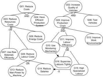
Qualitative goal analysis in Tropos starts with a num-ber of top goals and each of them is refined by decomposi-tion (AND or OR) into subgoals. For example, consider to model the strategic objectives of a production department in a vehicles company and suppose to have as main goals
Figure 1. Goal Model for the Vehicle Produc-tion Department
to reduce costs and to increase quality of vehicles (Fig. 1). The goal reduce costs (G1) is AND-decomposed into
re-duce resources costs (G3) and have efficient production
sys-tem (G4). Next, reduce resources costs (G3) can be
OR-decomposed into use raw materials effectively (G7), reduce
labour costs (G8), and reduce energy costs (G9), moreover
the goal reduce labour costs (G8) can be satisfied either by
reduce man-power (G13) or reduce salaries (G14). This
de-composition and refinements will continue until the goals are not considered tangible goals, i.e., when there is an ac-tor that can fulfil the goal.
Moreover, Tropos goal analysis allows us to model the influence of the satisfaction (denial) of a goal to the satisfac-tion (denial) of other goals. This influence can be positive or negative and is graphically indicated by “+/−” contribu-tion relacontribu-tions. Tropos also has “++” and “−−” to express strong positive contribution and strong negative contribu-tion, respectively. For example, the goal use monitoring mechanism (G10) in the production system will help in
en-forcing (“+” contribution) the goal of supervising labour (G16).
There are situations in which we need to model only the influence of the satisfaction of a goal on the denial (or the satisfaction) of another goal. For instance, having high spe-cialised labour (G15) impacts negatively to the satisfaction
of the goal reduce salaries (G14), but we cannot say
any-thing about what happen if the goal high specialised labour is denied. In other words we want to separate the effects ofSATandDENof the source node on theSATandDENof the target node. To model such situations, Tropos proposes to use different type of contribution links, namely−S,+S,
has partial evidence of being denied. Conversely, the denial of G15does not infer that G14will have partial evidence of
being satisfied.
The semantics of Tropos goal models is expressed by a set of basic axioms in [7]. For instance, the axioms state that full satisfiability (or deniability) implies partial satisfia-bility (or deniasatisfia-bility); for an “and” relation implies that the full and partial satisfiability of the target node require re-spectively the full and partial satisfiability of all the source nodes; for a “+S” relation, the axiom states that only the
partial satisfiability (but not the full satisfiability) propa-gates through a “+S” relation. Thus, e.g., an “and”
rela-tion propagates the minimum satisfiability value (and the maximum deniability one), while a “+S” relation
propa-gates at most a partial satisfiability value. To this extent, a “+S” relation can be seen as an “and” relation with an
unknown partially satisfiable goal. Similar considerations hold for the other relations. The axioms show also the rela-tions monotonically increase the values of satisfaction and denial among goals, namelySATandDENof sources nodes monotonically increaseSATandDENof target nodes. Max-imum function is used to combine different contributions.
Tropos provides also two forms of qualitative reasoning1
on goal models: forward [7] and backward [8] reasoning. Forward reasoning starts with assigning initial goal labels (SATandDEN) to a set of goals (typically leaf goals), then propagates the labels to the other goals of the model fol-lowing the relations of the axioms. This form of reasoning allow us to understand the effects of a particular goal as-signment over the whole model. It is useful for example to evaluate whether the assignment allows us to satisfy the stakeholders’ top goals or not. On the other hand, backward reasoning works in the opposite direction. The reasoning starts defining desired values of evidence for a number of goals (typically top goals) and constraints (i.e., the level of conflict that is accepted for the goal model, minimum evi-dence value of certain goal), then the reasoning tries to find an assignment for leaf goals (input goals) that can satisfy the desired values. The reasoning is enhanced by a number of criteria (e.g, minimum-cost [8]) to evaluate and choose among all the possible solutions. Backward reasoning is useful to find a possible assignment for leaf goals that satis-fies the stakeholders’ top goals.
3
Extending Goal Model for Risk
Manage-ment
As said, Tropos does not consider external events in the requirements analysis phase and it is not possible to analyse the effects of unpredictable situations on the stakeholders’
1Actually, Tropos proposes also quantitative reasoning mechanisms [7,
8]
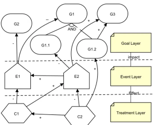
Figure 2. Extended Goal Model
goals. In this section, we extend the Tropos goal model in-troducing the new primitives event and treatment. Roughly, a risk is an event that has a negative impact on the satisfac-tion of a goal, while a treatment is a countermeasure that can be adopted in order to mitigate the effects of the risk.
In our framework we adopt the WordNet2 definition for
event:
• something that happens at a given place and time; • a special set of circumstances;
• a phenomenon located at a single point in space-time; • a consequence; i.e., a phenomenon that follows and is
caused by some previous phenomena.
An event becomes a risk when it produces a negative ef-fect, whereas it is an opportunity when it produces posi-tive effects. Probabilistic Risk Assessment (PRA) [12] has identified two mandatory properties for risk: likelihood and severity. Conversely, in our framework we consider like-lihood as a property of the event, whereas severity/impact is introduced as a contribution relation (negative/positive) between an event and a goal. This allows us to model situ-ations where a single event impacts on more than one goal. Adopting the idea of three-layers analysis of Defect De-tection and Prevention (DDP) [6], we consider three differ-ent layers in goal models Fig. 2. The strategic interests of the stakeholders are modelled in the first-layer (goal layer) using the classical Tropos goal model approach. Subse-quently, risks and opportunities that result relevant for the goal layer, are analysed in the second-layer (event layer), whereas countermeasures to mitigate risks are introduced and analysed in the third-layer (treatment layer). Graphi-cally, we represent an event as a pentagon (same representa-tion used in Fault Tree Analysis (FTA) [18]) and a treatment
2http://wordnet.princeton.edu/
as a task (no conceptual distinction between task [4] and treatment). As for goals, events and treatments can be de-composed in sub-events and sub-treatments and related by contribution relations to other goals, events, and treatments. Intra-layer and inter-layer relations [9] are fully adopted in the framework to capture all possible situations. The com-plete meta-model of the goal model is presented in Fig. 2
3.1
Event Layer
Based on the definitions in WordNet, we resume that an event can be a circumstance (e.g., “It rains”, “There is a war”), the outcome of the satisfaction of a goal or the out-come of the accomplishment of a task. In our framework, a risk is defined as an uncertain event with negative impact. This notion is slightly different from threat [13] in com-puter security and hazardous condition in reliability engi-neering [11], which are only defined as a potential circum-stance that could cause harm or loss and not specifying the notion of likelihood.
Events can be identified applying different approaches, such as obstacle analysis in KAOS [17], Taxonomy-base risk identification [5], or Risk in Finance [10]. Afterwards, an event is analysed by a decomposition into sub-events un-til each leaf event can be considered an independent event. Leaf events are used later to find proper countermeasures.
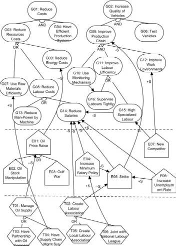
An event can influence more than one goal. So for ex-ample, in Fig. 3 the event strike (E5) obstructs the
satis-faction of reducing salaries (G14) because in this
circum-stance labours can demand an increment of the salary. On the other hand, it also obstructs the goal improve produc-tion chain (G5) since it can compromise and slow down the
production. An event can be considered as a risk for certain goals and at the same time an opportunity for other goals. For instance, the event have a new competitor (E7) is a risk
that obstructs the achievement of the goal high specialised labour (G15) because the competitor can offer better
con-ditions to the labour. However, the event can also be seen as an opportunity for the goal improve work environment (G12), because it gives more motivations to the employees
to compete with other companies.
As we already said an event can be characterised by two properties : likelihood and severity/impact. Likelihood is defined as how likely an event occurs [1]. In our frame-work, we represent likelihood by the level of evidence that supports and prevents the occurrence of the event (SATand
DEN). We adopt forSATandDENof an event the same Tro-pos meaning ofSATandDENfor a goal.
By impact, we mean the influence of an event to the goal fulfilment. This definition is similar to the definition given in DDP [6] and to the definition of severity in FMECA [1]. We classify impact as follows:
• Strong Positive(++) - the event occurrence gives a
strong contribution of the goal satisfaction;
• Positive(+) - the event occurrence gives a fair contri-bution of the goal satisfaction;
• Negative(−) - the event occurrence gives a fair con-tribution of the goal denial;
• Strong Negative(−−) - the event occurrence gives a strong contribution of the goal denial.
Since the effect of an event obstructs a goal only when it occurs (i.e., denial of an event does not give any impacts), in our model we use only rS relations, i.e., ++S, +S,−S,
and−−S, between an event and goals.
Figure 3. Extended Goal Model for the Vehicle Production Department
3.2
Treatment Layer
Once the events have been analysed, the analyst identi-fies and analyses the countermeasures to be adopted in order
to mitigate the risks. The mitigation of a risk can be realised in two different ways: reducing the likelihood or reducing the impact. However, in Tropos goal model it is not possi-ble to model a relation between a node and a relation (only between nodes), so in this paper we do not consider the re-duction of the impact as a possible mitigation. This will be part of our future work.
Similarly to goals and events, for countermeasures we useSATandDENto represent the evidence that supports and prevents the action. A countermeasure has effect on the event layer, and in particular over risks. We represent the effectof a countermeasure as a relation, where its strength is expressed by the sign of the contribution relations. As for events, we are interested to the propagation of the evidence for the success of a countermeasure (SAT) and therefore we limit the relations between countermeasures and events to rS relations. A countermeasure mitigates a risk when it
adds (propagates) evidence for its denial.
In our model we also allow for relations between the treatment layer and the goal layer. This is useful to model situations where a countermeasure adopted to mitigate a risk has also a contribution (especially negative) to some goals. For instance in Fig. 3, the countermeasure create a labour association (T2) can mitigate the likelihood of the
event strike (E5) – of course this is not always true.
How-ever, the association can have a better bargaining power w.r.t. the individual worker and obtain an increment of the salaries. This produces a negative effect on the satisfaction of the goal reduce salaries (G14).
3.3
Meta-model
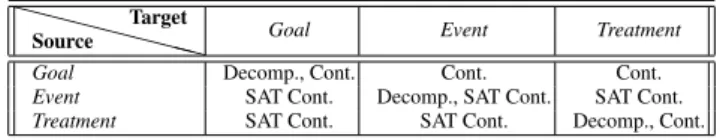
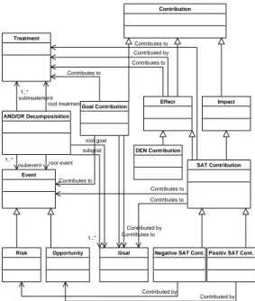
Table 1 resumes all the possible relations among goals, events, and treatments. For instance, the possible rela-tions form an event to other events are decomposition and
SAT contribution relations. Basically, all objects (Goal, Event, Treatment/Task) can be operated with all type of decomposition and contribution relations among the ob-jects in the same layer. Moreover, the only relation that can be used across the layers is the contribution relation. For events and treatments, there are limitations in the type of the contribution relations (only SAT-Relation; rS ∈
{++S, +S,−−S,−S}) as shown in the meta-model
rep-resented in Fig. 4. In the following we describe some situ-ations that could be modelled with cross layer contribution relations3:
goal→ event to model that a goal increases/reduces the occurrence of an event. For instance, the goal give big annual bonus can reduce the likelihood of strike; goal→ countermeasure to model that a goal
sup-ports/prevents the countermeasure accomplishment.
3Including impact-contribution and effect-contribution
XXXXXSource XX Target
Goal Event Treatment
Goal Decomp., Cont. Cont. Cont.
Event SAT Cont. Decomp., SAT Cont. SAT Cont.
Treatment SAT Cont. SAT Cont. Decomp., Cont.
Table 1. Relations in the Extended Goal Model
Decomposition r∈ {and, or}, Contribution r ∈ {++, +, −−, −}, SAT Contribution rS∈ {++S, +S,−−S,−S}
For instance, the achievement of the goal have a close partnership with the oil company helps to manage oil supply in the company;
event→ goal to model risk, namely the impact of event on the goal satisfaction. For instance, the event oil price raise can obstruct the satisfaction of the goal reduce energy costs;
event→ treatment to model the influence of the occur-rence of an event on the countermeasure accomplish-ment. For example, the event gulf war can make the oil very precious s.t. the oil company feels no need to have partnership with any end-customers;
treatment→ goal to model the side effect (negative or positive) of a countermeasure on the goal layer. For example, the countermeasure have a supply manage-ment system has a positive impact to the satisfaction of the goal use raw materials efficiently.
treatment→ event to model the effect of a countermea-sure to the mitigation of a risk. For example, having a good managing oil supply can mitigate the risk oil price raise;
4
Risk Analysis
As already discussed in the introduction, we intend to support the analyst in evaluating different requirements al-ternatives with respect to risk. In this section, we describe the methodological process and the qualitative reasoning mechanisms that are used in the different steps of the pro-cess.
The analysis process is described in the Algorithm 1 and consists of the following three steps:
1. find the alternative solutions (line 2-3),
2. evaluate each alternative against the relevant risks (line 8-10)
3. assess the countermeasures to mitigate the risks (line 11-16).
Goal Treatment Event Contribution AND/OR Decomposisition Opportunity Risk Impact Goal Contribution Effect
Positiv SAT Cont. DEN Contribution
Negative SAT Cont. SAT Contribution 1..* subtreatement root treatment 1..* subevent 1..* subgoal Contributes to Contributes to Contributes to root goal Contributes to Contributed by Contributed by Contributed by Contributed by Contributes to Contributes to Contributes to root event
Figure 4. Meta-model of the Extended Goal Model
The process starts taking in input the extended goal model and a set of desired values for top goals (i.e., sat-isfaction values-SATand acceptable risk values-DEN), and a number of goals as possible candidates for the final solution (input goals). For instance, we may desire to fully satisfy G1(Sat(G1)=F) without any risk (Den(G1)=N).
Backward Reasoning (line 2) generates a set of pos-sible assignment values for the input goals that can satisfy the desired values. We use the standard Tropos backward reasoning limited to the goal layer (i.e., not considering the relations with the other two layers) and not considering any constraints. So for instance, in order to fully satisfy G1we
can either fully satisfy{G7, G4}, {G13, G4} or {G14, G4}.
The analyst chooses a subset of the alternatives on the basis of a certain criteria (i.e., minimum-cost [8], softgoals) called candidate solution (line 3). The rest of the process will be limited to the analysis of this subset. For instance, the analyst can decide to choose the alternatives{G13, G4}
and{G14, G4} considering the goal use raw materials (G7)
is too expensive.
Each candidate solution is now evaluated against risks and then necessary countermeasures are intro-duced (line 4-18). First, the analyst checks whether the candidate solution needs countermeasures to ob-tain the desired values in the top goals. If not the candidate solution is added directly to the solution and its cost is calculated (line 6). Otherwise, countermeasures must be introduced in the candidate solution (line 8-16).
So for example, evaluating{G13, G4} we see from Fig. 3
that there is no risk associated to them so we do not need any countermeasure. It is different for{G14, G4}.
In order to define the countermeasures, we first need to calculate the risk values that are acceptable for the stakeholders. In other words, we need to find the maxi-mum assignable values of risk that produce an acceptable
DEN value for top goals. So for example, in our exam-ple we need to find a set of countermeasures able to mit-igate risks s.t. Den(G1)=N. To do this we need to
con-sider only the relevant risks for the candidate solution, namely risks that have an impact on the input goals and goals reachable from them by decomposition (“re-lated goals”). For instance, since the related goals of {G14, G4} are {G14, G8, G3, G4, G1} we consider only the
risks{E4, E5}.
Algorithm 1Risk Analysis Process
Ensure: analyse risk for each alternative solutions and find necessary
countermeasures to ensure the satisfaction of top goals.
Require: goal model hG, Ri , label array top goals, node array
in-put goals, label array events
1: solution array solution{solution that has already encompassed risks
and necessary countermeasures}
2: alt solution←Backward Reasoning(hG, Ri , nil,
top goals, input goals)
3: candidate solution←Select Can Solution(candidate solution)
{alt solution ⊆ candidate solution}
4: for all Si∈ candidate solution do
5: if Satisf y(hG, Ri , top goals, hSi, events, nili) then
6: add(solution,hSi, nill, Calc Cost(Si, nil)i)
7: else
8: boolean array Related Goals←
Related Goals(hG, Ri , Si)
9: labels←Standard F orward Reasoning(hG, Ri , Si)
10: acc events←Calc Event(labels, related goals, events)
11: nec treatment←Backward Reasoning(hG, Ri , events,
acc events, avail treatment)
12: for all Tj∈ nec treatment do
13: if Satisf y(hG, Ri , top goals, hSi, events, Tji) then
14: add(solution,hSi, Tj, Calc Cost(Si, Tj)i)
15: end if
16: end for
17: end if
18: end for
Standard F orward Reasoning (line 9) is used to propagate the input values of the candidate solution in the model and so evaluate the impact of the risk. Once we have an assignment for all the goals of the model we can cal-culate the acceptable values for the event (i.e., values that can still satisfy the desired top goals). This is done by the Calc Event Algorithm 5. We illustrate it later.
Backward reasoning is again applied (line 11) to find possible treatments that can guarantee the acceptable risk (acc event). Of course, we can have more than one pos-sible combination of treatments. For instance, defining Sat(E4)=P, Den(E4)=F and Sat(E5)=F, Den(E5)=F as
hhhhhhhhSat(E)
Den(E) Full Partial
Full Sat(E) = N, Den(E) = N Sat(E) = P, Den(E) = N
Partial Sat(E) = N, Den(E) = P Sat(E) = N, Den(E) = N
Table 2. Conflict Resolution for Events
or{T6} as possible treatments.
Finally (line 12-16), each set of treatments are evaluated with respect to the initial desired values (indeed, there could be the case that a treatment has negative contribution di-rectly to the goal layer) and the affordable costs. To do this we use again the Satisf y algorithm (line 13) that basically consists of the following three steps:
1. the input values for goal, events and treatments are propagated over the whole model;
2. conflicts in the event layer are solved ;
3. the input values for goals, treatments, events (as results of step 2) are propagated excluding incoming relations to events.
For the three steps, we use the N ew F orward Reasoning (Algorithm 2), which is a revised version of the algorithm presented in [7]. The main difference is that here we extend the propagation to the event and the treatment layer and we introduce the conflict resolution step. As discussed in the previous section, the influence of a risk on a goal depends on the
SAT value of the risk and a mitigation corresponds to the increment of the level of the DEN. For example, the impact of E5 on the goal G14 depends on the SATvalue
(e.g.,Sat(E5)=F), and the effect of T5on G14is to increase
theDENvalue of E5(e.g., Den(E5)=F). A countermeasure
is effective when it is able to generate a conflict between
SATandDENin the risk. For example, after taking T5there
is a conflict in E5(i.e., Sat(E5)=F and Den(E5)=F). The
conflict resolution step allows us to separate the effects of the countermeasures on the goal layer from the impact of the risks. Table 2 presents the conflict resolution rules we adopted.
Algorithm 2New Forward Reasoning
Ensure: propagate evidence to the goal model
Require: goal modelhG, Ri , label array initial
1: resolution←false
2: pre res←
Label P ropagation(hG, Ri , initial, resolution)
3: post res←Resolve Conflict(hG, Ri , initial, pre res)
4: resolution←true
5: result←Label P ropagation(hG, Ri , post res, resolution)
6: return result
Calc Event algorithm (Algorithm 5) basically does the reverse of conflict resolution and distinguishes between risk
Algorithm 3Label Propagation
Require: goal modelhG, Ri , label array initial, boolean resolution
1: label array current, old 2: current = initial
3: while old6= current do
4: old←current
5: for all Ni∈ G do
6: if not (resolution and Is Event(Ni)) then {checking
whether conflict resolution has already applied at events or not}
7: current[i]←Update Label(i, hG, Ri , old)
8: end if
9: end for
10: end while 11: return current
Algorithm 4Update Label
Require: int i, goal modelhG, Ri , label array old
1: for all Rj∈ R s.t. target(Rj) = Nido
2: satij= Apply Rules Sat(Ni, Rj, Old)
3: denij= Apply Rules Den(Ni, Rj, Old)
4: end for
5: return {max(max array(satij), Old[i].sat),
max(max array(denij), Old[i].den)}
Algorithm 5Calc Event
Ensure: calculate acceptable value of risks s.t the input goals can satisfy top goals
Require: label array goals, label array events, boolean array
re-lated goals
1: acceptable events←events
2: for all Bi∈ related goals do
3: if Bithen
4: for all (Rj ∈ R s.t. target(Rj) = goalsi) and
Is Event(source(Rj)) do 5: node←source(Rj)
6: k←Node Index(source(Rj))
7: if (Rj∈ {−S,−−S}) and goalsi.den < node.sat then
{risk}
8: if goalsi.den = N and node.sat = F then
9: acceptable eventsk.den←F
10: else if (goalsi.den = N and node.sat = P ) or
(goalsi.den = P and node.sat = F ) then
11: acceptable eventsk.den←P
12: end if
13: else if (Rj ∈ {+S, ++S}) and goalsi.sat > node.sat
then{opportunity}
14: if goalsi.sat = P and node.sat = N then
15: acceptable eventsk.sat←P
16: else if goalsi.sat = F then
17: acceptable eventsk.sat←F
18: end if
19: end if
20: end for
21: end if
22: end for
23: return acceptable events
Figure 5. Risk Analysis Tool
and opportunity events, line (8-12) and line(14-18), re-spectively. For example, since we want no risk on G14
(Den(G14)=N) but E4andE5produce a partial denial, we
need to introduce countermeasures so create a conflict s.t. E4and E5do not impact on G14. In this case, Calc Event
produces the acceptable values of risk Den(E4)=P and
Den(E5)=F to neutralise the Sat(E4)=P and Sat(E5)=F.
As final result of the process we obtain all the possible solutions (among the candidate solution) that can satisfy the initial requirements and costs associated to them. Now, the analyst can decide which solution to adopt.
5
Tool and Experimental Results
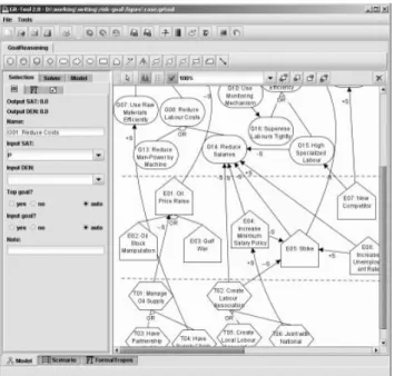
In this section, we briefly present the tool we have devel-oped and some experimental results obtained with it.
The tool is an extension of the Goal Reasoning Tool4
(GR-Tool) developed within the Tropos project. Basically, the tool (Fig. 5) is graphical tool in which it is possible to draw the extended goal models and run the algorithms and tools for (standard and new) forward and backward rea-soning. The algorithms presented in Section 4 have been fully developed in JAVA and are embedded in the tool. For their implementation we started from the GR-Tool reason-ing mechanisms and we have re-implemented them intro-ducing the necessary modifications as described in Sec-tion 4. For more details about the GR-Tool and its extension we suggest to visit the Tropos web page.
4http://sesa.dit.unitn.it/goaleditor/
Input Goal Cost S1 S2 S3 S4 S5 S6 S7 S8 G04: Have Eff. Prod. Sys. 6 X X X X X X X X G06: Test Vehicles 4 X X X X X X X X G07: Use Raw Materials Eff. 4.5 X X G09: Reduce Energy Costs 3 X X
G10: Use Mon. Mechanism 5 X X X X X X X X G12: Improve Work Env. 6 X X X X X X X X G13: Reduce Man-Pow. by Mach. 9 X X G14: Reduce Salaries 3.5 X X
G15: High Specialized Lab. 7 X X X X G16: Supervise Lab. Tightly 3.5 X X X X
Total Cost 27.5 28 29 31 31.5 32.5 33.5 37
Table 3. Cost of Alternative Solutions
To test our approach and its implementation we run a number of experiments for the case of the Production De-partment of a Vehicles Company presented in Fig. 3.
Table 3-5 summarise an example of these results. Sup-pose we want to obtain a partial satisfaction of goal G1
(re-ducing cost), a fully satisfaction of G2 (increasing quality
of vehicles), and avoid any risk on them. So we have as in-put{Sat(G1)=P, Sat(G2)=F, Den(G1)=N, Den(G2)=N}.
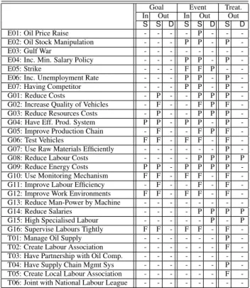
Executing Backward Reasoning we find a set of possi-ble solutions (as reported in Tapossi-ble 3) and we select among them the cheapest one S1. The total cost of each solution is calculated summing up the costs of the single input goals. Of course, other criteria can be adopted for the selection of the solution. As discussed in [8], for instance we could also evaluate the effects of the solution over some qualities (softgoals). Forward reasoning is applied then to calculate the effects of the selected solution to the other goals of the model (column “Goal-Out” Table 4).
Now, let suppose we have evidence about the occurrence of some of the events and want to see the impact of them on the goal layer. For example, considering the event as-signment reported in column “Event-In” (i.e., Sat(E2)=P,
Sat(E4)=P, Sat(E5)=F, Sat(E6)=P, Sat(E7)=P), we
ob-tain that (“Event-Out”) top goals G1and G2 are both
par-tially satisfied and denied. In order to re-obtain the desider-ate values for top goals we need to find necessary treatments able to mitigate the risks. There are four possible counter-measure sets that could be taken to mitigate the risks (see Table 5) and the total cost of countermeasures can be cal-culated summing up the single cost of input treatments. In this experiment, we adopt C2 (i.e., Sat(T4)=P, Sat(T5)=F)
based on their costs and their side effects. Even C2 is the most expensive, it is worth enough compared with T4
pos-itive contribution to G7 and both treatments do no agitate
the risks (conversely, T6triggers the risk E4). Finally, the
tool generates the final configuration with input S1 and C2 (in column ”Treatment-Out”) where our desired values for top goals are again obtained.
Let suppose we take the second cheapest solution S2. The “relevant-risks” for this alternative solution are E4, E5,
Goal Event Treat. In Out In Out Out S S D S S D S D E01: Oil Price Raise - - - - P - - -E02: Oil Stock Manipulation - - - P P - P -E03: Gulf War - - - -E04: Inc. Min. Salary Policy - - - P P - P
-E05: Strike - - - F F P -
-E06: Inc. Unemployment Rate - - - P P - P -E07: Having Competitor - - - P P - P -G01: Reduce Costs - P - - P P P -G02: Increase Quality of Vehicles - F - - F P F -G03: Reduce Resources Costs - P - - P P P -G04: Have Eff. Prod. System P P - P P - P -G05: Improve Production Chain - F - - F P F -G06: Test Vehicles F F - F F - F -G07: Use Raw Materials Efficiently - - - P -G08: Reduce Labour Costs - - - - P P P P G09: Reduce Energy Costs P P - P P P P -G10: Use Monitoring Mechanism F F - F F - F -G11: Improve Labour Efficiency - F - - F - F -G12: Improve Work Environments F F - F F - F -G13: Reduce Man-Power by Machine - - - -G14: Reduce Salaries - - - - P P P P G15: High Specialised Labour - - - P - P G16: Supervise Labours Tightly F F - F F - F -T01: Manage Oil Supply - - - P -T02: Create Labour Association - - - F -T03: Have Partnership with Oil Comp. - - - -T04: Have Supply Chain Mgmt Sys - - - P -T05: Create Local Labour Association - - - F -T06: Joint with National Labour League - - -
-Table 4.SAT-DENvalues in Risk Analysis of S1 Treatment Input Cost S1 S2
C1 C2 C3 C4 C5 C6 T03: Have Partnership with Oil Comp. 6 X X
T04: Have Supply Chain Mgmt Sys 8 X X T05: Create Local Labour Association 6 X X X T06: Joint with National Labour League 5 X X X
Total Cost 12 14 11 13 6 5 Table 5. Cost of Possible Treatments
necessary to be taken are T5or T6. Among the two, even if
more costly, T5results to be better than T6since it does not
have any effects on the events’ occurrence (T6 has a “+S”
contribution on E4). Comparing the alternatives, we can
conclude taking S2 and C5 is cheaper than S1 and C2 and moreover S2 is less risky than S1 (i.e., the risks of S2⊂ the risks of S1). Similar consideration can be done for the other solutions.
6
Related Work
The most relevant works in literature that have similar-ities with our approach are KAOS and DDP . We briefly discuss them in the following.
KAOS [16] is the methodology that provides a specifica-tion by capturing why, who, and when aspects in addispecifica-tion to what aspect in requirements. KAOS, moreover, has already been extended beyond goals, by defining obstacles which can be seen as boundaries in requirement analysis. An
ob-stacle is defined as an undesirable behaviour to the strate-gic interests of stakeholders which can be used to model the risk. In [16], they demonstrate how to derive the ob-stacles from the goal structure and to ensure the complete-ness of obstacles with respect to the goal structure and its domain. This technique assumes a complete knowledge to define the domain of the goal, which is hardly to meet in the reality. Conversely, Tropos defines the axioms as “at least” premises which assume there are not complete knowledge to define the number of evidence. The methodology, also, introduces the guidance for defining obstacle resolution to mitigate and, possibly, eliminate the obstacle. Though we can represent a risk as an obstacle, two mandatory proper-ties of risk (likelihood and severity) are still missing. How-ever, the obstacle concept and all related analysis (obstacle identification, obstacle resolution) could be used as a basis for the further enhancement of our framework.
DDP [6] is a model that is developed and applied in Jet Propulsion Lab. and NASA. DDP consists of three layers model (Objectives, Risks, Mitigation). In this model, each objective has a weight to represent its importance. A risk has a likelihood of occurrence and a mitigation has a cost for accomplishment (namely resource consumption). Severity of the risk is represented by impact relation between objec-tive and risk. Moreover, DDP model specifies how to com-pute the level of objectives achievement and the cost of mit-igation5from a set of taken mitigation. This calculation
al-lows us to evaluate the impact of taken countermeasures and thus supports the decision making process. The DDP model also allows us to work together with other quantitative tools (FMECA [1], FTA [18]) to model and assess risk/failure. In [6], they demonstrate how to integrate FMECA and FTA into DPP model. There are some differences between the concept of objective [6] and the concept of goal in oriented requirement engineering [4, 16, 19, 2]. In goal-oriented, the goal has a structure (e.g., tree, graph). Con-versely, DDP depicts objective (also risk and mitigation) as a solitary object (i.e., there is no relation among objects in the same layer). This feature could limit in modelling sit-uations (e.g., domino effect [14]) in which the occurrence of a risk can increase/decrease the likelihood of other risks. DDP model allows us only to establish relations between layers (i.e., risks to goals, mitigation to risk) which is not enough to represent all possible situations. For example, there could be cases where a treatment affect also the sat-isfaction of some objective. Our framework adopts and en-hances the idea of three-layers model.
7
Conclusions and Future Work
In this paper, we have presented a framework to model and reason about risk within the requirements engineering
5objective restoration categories as one kind of mitigation action
process. We have adopt and extended the Tropos goal mod-elling framework and proposed qualitative reasoning algo-rithms to analyse risk during the process of evaluation and selection of alternatives. However, our approach has some limitations that we want to overcome as part of our fu-ture work. Specifically, as discussed in the paper our mod-elling framework supports only relationships between nodes (goals, events, tasks) and this could be a limitation when we want to model situations where a treatment mitigates the risk reducing its impact on the goal layer. In other words, we need to extend the framework introducing the possibility to establish relations also between nodes and arcs. Another limitation is related to the fact that in our framework the val-ues forSATandDENcan only increase monotonically and it is not possible to model the fact that an event decreases the evidence for the satisfaction of a goal. Finally, as done for goal models we want to propose also quantitative reasoning mechanisms where evidence is expressed in term of proba-bility.
Acknowledgement
This work has been partly supported by the projects EU-SENSORIA, EU-SERENITY, FIRB-ASTRO, PAT-MOSTRO, PAT-STAMPS.
References
[1] Military Standard, Procedures for Performing a Failure
Mode, Effects, and Critical Analysis (MIL-STD-1692A). US
Department of Defense, 1980.
[2] A. I. Anton. Goal-Based Requirements Analysis. In
ICRE ’96: Proceedings of the 2nd International Conference on Requirements Engineering, page 136, Washington, DC,
USA, 1996. IEEE Computer Society.
[3] B. W. Boehm. Software Risk Management: Principles and Practices. IEEE Software, 8(1):32–41, 1991.
[4] P. Bresciani, A. Perini, P. Giorgini, F. Giunchiglia, and J. Mylopoulos. Tropos: An Agent-Oriented Software Devel-opment Methodology. Autonomous Agents and Multi-Agent
Systems, 8(3):203–236, 2004.
[5] M. J. Carr, S. L. Konda, I. Monarch, and F. C. Ulrich.
Taxonomy-Based Risk Identification. Technical Report
CMU/SEI-93-TR-6, ESC-TR-93-183, Software Engineer-ing Institute, Carnegie Mellon University, June 1993. [6] M. S. Feather. Towards a Unified Approach to the
Repre-sentation of, and Reasoning with, Probabilistic Risk Infor-mation about Software and its System Interface. In 15th
IEEE International Symposium on Software Reliability En-gineering, pages 391–402. IEEE Computer Society,
Novem-ber 2004.
[7] P. Giorgini, J. Mylopoulos, E. Nicchiarelli, and R. Sebas-tiani. Formal Reasoning Techniques for Goal Models.
Jour-nal of Data Semantics, October 2003.
[8] P. Giorgini, J. Mylopoulos, and R. Sebastiani. Simple and Minimum-Cost Satisfiability for Goal Models. In CAISE
’04: In Proceedings International Conference on Advanced Information Systems Engineering, volume 3084, pages 20–
33. Springer, June 2004.
[9] P. Giorgini, J. Mylopoulos, and R. Sebastiani. Goal-Oriented Requirements Analysis and Reasoning in the Tro-pos Methodology. Engineering Applications of Artifcial
In-telligence, 18(2):159–171, March 2005.
[10] G. A. Holton. Defining Risk. Financial Analyst Journal, 60(6):1925, 2004.
[11] R. R. Lutz and R. M. Woodhouse. Requirements Analysis Using Forward and Backward Search. Annals Software
En-gineering, 3:459–475, 1997.
[12] NASA. Probabilistic Risk Assessment
Proce-dures Guide for NASA Managers and Practitioners. http://www.hq.nasa.gov/office/codeq/, August 2002. [13] C. P. Pfleeger and S. L. Pfleeger. Security in Computing.
Prentice Hall PTR, 3rd edition, 2002.
[14] G. Reniers, W.Dullaert, and K. Soudan. A domino effect evaluation model. Working papers, University of Antwerp, Faculty of Applied Economics, December 2004.
[15] G. G. Roy and T. L. Woodings. A framework for risk analy-sis in software engineering. In APSEC ’00: Proceedings of
the Seventh Asia-Pacific Software Engineering Conference,
page 441, Washington, DC, USA, 2000. IEEE Computer So-ciety.
[16] A. van Lamsweerde and E. Letier. Handling Obstacles in Goal-Oriented Requirements Engineering. IEEE
Transac-tion Software Engineering, 26(10):978–1005, 2000.
[17] A. van Lamsweerde, E. Letier, and R. Darimont. Managing Conflicts in Goal-Driven Requirements Engineering. IEEE
Transaction Software Engineering, 24(11):908–926, 1998.
[18] W. Vesely, F. Goldberg, N. Roberts, and D. Haasl. Fault Tree
Handbook. U.S Nuclear Regulatory Commission, 1981.
[19] E. Yu. Modelling Strategic Relationships for Process
Engi-neering. PhD thesis, University of Toronto, Department of