UNIVERSITY
OF TRENTO
DEPARTMENT OF INFORMATION AND COMMUNICATION TECHNOLOGY
38050 Povo – Trento (Italy), Via Sommarive 14
http://www.dit.unitn.it
A NEW SEARCH ALGORITHM FOR FEATURE SELECTION IN
HYPERSPECTRAL REMOTE SENSING IMAGES
Sebastiano B. Serpico and Lorenzo Bruzzone
2001
A New Search Algorithm for Feature Selection in
Hyperspectral Remote Sensing Images
Sebastiano B. Serpico(*), Senior Member, IEEE, andLorenzo Bruzzone(o),Member, IEEE (*) Dept. of Biophysical and Electronic Engineering, University of Genoa
Via Opera Pia, 11 A, I-16145, Genova, Italy E-mail: [email protected]
(o) Dept. of Information and Communication Technologies, University of Trento
Via Sommarive, 14, I-38050, Trento, Italy E-mail: [email protected]
Abstract - A new suboptimal search strategy suitable for feature selection in very high-dimensional remote-sensing images (e.g. those acquired by hyperspectral sensors) is proposed. Each solution of the feature selection problem is represented as a binary string that indicates which features are selected and which are disregarded. In turn, each binary string corresponds to a point of a multidimensional binary space. Given a criterion function to evaluate the effectiveness of a selected solution, the proposed strategy is based on the search for constrained local extremes of such a function in the above-defined binary space. In particular, two different algorithms are presented that explore the space of solutions in different ways. These algorithms are compared with the classical sequential forward selection and sequential forward
floating selection suboptimal
techniques, using hyperspectral remote-sensing images (acquired by the AVIRIS
sensor) as a data set. Experimental results point out the effectiveness of both
algorithms, which can be regarded as valid alternatives to classical methods, as
they allow interesting tradeoffs between the qualities of selected feature subsets
and computational cost.
Keywords: feature selection, hyperspectral data, search algorithms, remote sensing.
I. I
NTRODUCTIONThe recent development of hyperspectral sensors has opened new vistas for the monitoring of the earth’s surface by using remote sensing images. In particular, hyperspectral sensors provide a dense sampling of spectral signatures of land covers, thus allowing a better discrimination among similar ground cover classes than traditional multispectral scanners [1]. However, at present, a major limitation on the use of hyperspectral images lies in the lack of reliable and effective techniques for processing the large amount of data involved. In this context, an important issue concerns the selection of the most informative spectral channels to be used for the classification of hyperspectral images. As hyperspectral sensors acquire images in very close spectral bands, the resulting high-dimensional feature sets contain redundant information. Consequently, the number of features given as input to a classifier can be reduced without a considerable loss of information [2]. Such reduction obviously leads to a sharp decrease in the processing time required by the classification process. In addition, it may also provide an improvement in classification accuracy. In particular, when a supervised classifier is applied to problems in high-dimensional feature spaces, the Hughes effect [3] can be observed, that is, a decrease in classification accuracy when the number of features exceeds a given limit, for a fixed training-sample size. A reduction in the number of features overcomes this problem, thus improving classification accuracy.
Feature selection techniques generally involve both a search algorithm and a criterion function [2],[4],[5]. The search algorithm generates and compares possible “solutions”
of the feature selection problem (i.e. subsets of features) by applying the criterion function as a measure of the effectiveness of each considered feature subset. The best feature subset found in this way is the output of the feature selection algorithm. In this paper, attention is focused on search algorithms; we refer the reader to other papers [2],[4],[6],[7] for more details on criterion functions.
In the literature, several optimal and suboptimal search algorithms have been proposed [8]-[16]. Optimal search algorithms identify the subset that contains a prefixed number of features and is the best in terms of the adopted criterion function, whereas suboptimal search algorithms select a good subset that contains a prefixed number of features but that is not necessarily the best one. Due to their combinatorial complexity, optimal search algorithms cannot be used when the number of features is larger than a few tens. In these cases (which obviously include hyperspectral data), suboptimal algorithms are mandatory.
In this paper, a new suboptimal search strategy suitable for hyperdimensional feature selection problems is proposed. This strategy is based on the search for constrained local extremes in a discrete binary space. In particular, two different algorithms are presented that allow different tradeoffs between the effectiveness of selected features and the computational time required to find a solution. Such algorithms have been compared with other suboptimal algorithms (described in the literature) by using hyperspectral remotely sensed images acquired by the Airborne Visible/Infrared Imaging Spectrometer (AVIRIS). Results point out that the proposed algorithms represent valid alternatives to classical algorithms as they allow different tradeoffs between the qualities of selected feature subsets and computational cost.
The paper is organized into five sections. Section 2 presents a literature survey on search algorithms for feature selection. Sections 3 and 4 describe the proposed search
strategy and the two related algorithms. In Section 5, the AVIRIS data used for experiments are described and results are reported. Finally, in Section 6, a discussion of the obtained results is provided and conclusions are drawn.
II. P
REVIOUSW
ORKThe problem of developing effective search strategies for feature selection algorithms has been extensively investigated in pattern recognition literature [2],[5],[9], and several optimal and suboptimal strategies have been proposed.
When dealing with data acquired by hyperspectral sensors, optimal strategies cannot be used due to the huge computation time they require. As is well-known from the literature [2],[5], an exhaustive search for the optimal solution is prohibitive from a computational viewpoint, even for moderate values of the number of features. Not even the faster and widely used branch and bound method proposed by Narendra and Fukunaga [2],[8] makes it feasible to search for the optimal solution when high-dimensional data are considered. Hence, in the case of feature selection for hyperspectral data classification, only a suboptimal solution can be attained.
In the literature, several suboptimal approaches for feature selection have been proposed. The simplest suboptimal search strategies are the sequential forward selection
(SFS) and sequential backward selection (SBS) techniques [5],[9]. These techniques identify the best feature subset that can be obtained by adding to, or removing from, the current feature subset one feature at a time. In particular, the SFS algorithm carries out a “bottom-up” search strategy that, starting from an empty feature subset and adding one feature at a time, achieves a feature subset with the desired cardinality. On the contrary, the SBS algorithm exploits a “top-down” search strategy that starts from a complete set of features and removes one feature at a time until a feature subset with the desired
cardinality is obtained. Unfortunately, both algorithms exhibit a serious drawback. In the case of the SFS algorithm, once the features have been selected, they cannot be discarded; analogously, in the case of the SBS search technique, once the features have been discarded, they cannot be re-selected.
The plus-l-minus-r method [10] employs a more complex sequential search approach to overcome this drawback. The main limitation on this technique is that there is no theoretical criterion for selecting the values of l and r to obtain the best feature set.
A computationally appealing method is the max-min algorithm [11]. It applies a sequential forward selection strategy based on the computation of individual and pairwise merits of features. Unfortunately, the performances of such a method are not satisfactory, as confirmed by the comparative study reported in [5]. In addition, Pudil. et al. [12] showed that the theoretical premise providing the basis for the max-min approach is not necessarily valid.
The two most promising sequential search methods are those proposed by Pudil et al. [13], namely, the sequential forward floating selection (SFFS) method and the sequential backward floating selection (SBFS) method. They improve the standard SFS and SBS techniques by dynamically changing the number of features included (SFFS) or removed (SBFS) at each step and by allowing the reconsideration of the features included or removed at the previous steps.
The representation of the space of feature subsets as a graph (“feature selection lattice”) allows the application of standard graph-searching algorithms to solve the feature selection problem [14]. Even though this way of facing the problem seems to be interesting, it is not widespread in the literature.
The application of genetic algorithms was proposed in [15]. In these algorithms, a solution (i.e. a feature subset) corresponds to a “chromosome” and is represented by a
binary string whose length is equal to the number of starting features. In the binary string, a zero corresponds to a discarded feature and a one corresponds to a selected feature. Satisfactory performances were demonstrated on both a synthetic 24-dimensional data set and a real 30-24-dimensional data set. However, the comparative study in [16] showed that the performances of genetic algorithms, though good for medium-sized problems, degrade as the problem dimensionality increases.
Finally, we recall that also the possibility of applying simulated annealing to the feature selection problem has been explored [17].
According to the comparisons made in the literature, the sequential floating search methods (SFFS and SBFS) can be regarded as being the most effective ones, when one deals with very high-dimensional feature spaces [5]. In particular, these methods are able to provide optimal or quasi-optimal solutions, while requiring much less computation time than most of the other strategies considered [5],[13]. The investigation reported in [16] for data sets with up to 360 features shows that these methods are very suitable even for very high-dimensional problems.
III. T
HES
TEEPEST-A
SCENTS
EARCHS
TRATEGYLet us consider a classification problem in which a set X of n features is available to characterize each pattern:
X=
{
x1, …, xn}
. (1)The objective of feature selection is to reduce the number of features utilized to characterize patterns by selecting, through the optimization of a criterion function J (e.g. maximization of a separability index or minimization of an error bound), a good subset S
S=
{
s1, …, sm: si∈
X, i=1,..,m}
. (2)
The criterion function is computed by using a preclassified reference set of patterns (i.e. a training set); the value of J depends on the features included in the subset S (i.e.
J=J(S)).
The entire set of all feature subsets can be represented by considering a discrete binary space B. Each point b in this space is a vector with n binary components. The value 0 in the k-th position indicates that the k-th feature is not included in the corresponding feature subset; the value 1 in the j-th position indicates that the j-th feature is included in the corresponding feature subset. For example, in a simple case with m=4 features, the binary vector b=(0, 1, 0, 1) indicates the feature subset that includes only the second and fourth features:
b=(0, 1, 0, 1)
⇔
S={
x2, x4}
. (3)The criterion function J can be regarded as a scalar function defined in the aforesaid discrete binary space. Let us consider, without loss of generality, the case in which the criterion function has to be maximized. In this case, the optimal search for the best solution to the problem of selecting m out of n features corresponds to the problem of finding the global constrained maximum of the criterion function, where the constraint is defined as the requirement that the number of selected features be exactly m (in other words, the solution must correspond to a vector b with m components equal to 1 and (n-m) components equal to 0).
With reference to the above description of the feature selection problem, we propose to search for suboptimal solutions that are constrained local maxima of the criterion function. According to our method, we start from a point b0 corresponding to an initial
features which allow the value of the criterion function to be progressively increased. This strategy differs from most search algorithms for feature selection, which usually progressively increase (e.g. SFS) or decrease (e.g. SBS) the number of features in S, with possible “backtracking” (e.g. SFFS and SFBS).
We now need to give a precise definition of local maxima in the previously described discrete space B. To this end, let us consider the neighborhood of a vector b that includes all vectors that differ from b in no more than two components. We say that a vector b is a local maximum of the criterion function J in such a neighborhood if the value of the criterion function in b is greater than or equal to the value the criterion function takes on any other point of the neighborhood of b. We note that the neighborhood of any vector b
is made up of n vectors that differ only in one component, and of n
×
(n-1)/2 vectors that differ in two components. However, if b satisfies the constraint, only m×
(n-m) vectors included in the neighborhood of b still satisfy the constraint. Constrained local maxima are defined with respect to this subset of the neighborhood.The Steepest Ascent Algorithm
Symbol definitions
J(S) value of the feature selection criterion function computed for the feature subset S;
S0 feature subset utilized for the initialization;
Si best feature subset selected at the i-th iteration (i>0);
B discrete binary space representing the entire set of all feature subsets;
bi vector of n binary components that represents Si in the space B; Di set of features discarded by the search algorithm at the i-th iteration;
satisfies the constraint on the number of features to be selected;
Jmax maximum value of J found by the search algorithm by exploring
Ω
i-1 .Initialization
An initial feature subset S0, composed of m features selected from the set X of n
available features, is considered. The corresponding starting vector b0 in B can be easily obtained starting from S0. The discarded (n-m) features are included in the
complementary set D0:
D0=
{
si: si∈
X, si∉
So}
. (4)The value J(So) of the criterion function is computed for the initial subset So.
i-th Iteration
At the i-th iteration of the algorithm, all possible exchanges of one feature belonging to Si-1 for another feature belonging to Di-1 are considered and the
corresponding values of J are computed. This is equivalent to evaluating J in the set of vectors
Ω
i-1 corresponding to the portion of the neighborhood of bi-1 thatsatisfies the constraint. The maximum value obtained in this way is considered:
Jmax = max
{
J(S)}
S∈
Ω
i-1. (5)If the following relation holds:
Jmax > J(Si -1) (6)
then the feature exchange that results in Jmax is accepted and the subsets of features
Stop Criterion
When the condition
Jmax
≤
J(Si -1) (7)holds, it means that a local maximum has been reached; then the algorithm is stopped. Finally, Si is set to Si-1.
The name “steepest ascent” (SA) search algorithm derives from the fact that, at each iteration, a step in the direction of the steepest ascent of J, in the set
Ω
i-1, is taken. Thealgorithm is iterated as long as it is possible to increase the value of the criterion function. Convergence to a local maximum in a finite number of iterations is guaranteed. At convergence, Si contains the solution, that is, the selected subset of m features. The
algorithm can be run several times with random initializations (i.e. starting from different randomly generated feature subsets S0) in order to better explore the space of solutions (a
different local maximum may be obtained at each run). An alternative strategy lies in considering only one “good” starting point S0 generated by another search algorithm (e.g.
the basic SFS technique); in this case, only one run of the algorithm is carried out.
IV. A Fast Algorithm for a Constrained Search
We have also investigated other algorithms aimed at a constrained search for local maxima, in order to reduce the computational load required by the proposed technique. For the sake of brevity, we shall consider here only one of such search algorithms. To get an idea of the computational load of SA, we note that, at each iteration, the previously defined set of vectors
Ω
i-1 is explored to check if a local maximum has been reachedm
×
(n-m) points; the value of J is computed for each of them. Globally, the number of times required to evaluate J is:k
×
m×
(n-m) (8)where k is the number of iterations required. The fastest search algorithm among those we have experimented is the following “fast constrained search” (FCS) algorithm. This algorithm is based on a loop whose number of iterations is deterministic. For simplicity, we present it in the form of a pseudocode.
The Fast Constrained Search Algorithm
START from an initial feature subset S0 composed of m features selected from X
Set the current feature subset Sk to S0
Compute the complementary subset Dk of Sk
FOR each element si
∈
S0 FOR each element sj∈
DkGenerate Sij by exchanging si for sj in Sk
Compute the value J(Sij) of the criterion function CONTINUE
Set Ji,max to the maximum of J(Sij) obtained by exchanging si for any possible sj
IFJi,max>J(Sk), THEN update Sk by the exchange si
←
sj that provided Ji,maxCompute the complementary subset Dk of Sk ELSE leave Sk unchanged
CONTINUE
computational load equivalent to that of one iteration of the SA algorithm. By contrast,
the result is not equivalent, as, in this case, the number of moves in B can range from 1
to m (each of the features in
S0can be exchanged only once or left in
S0), whereas SA
performs just one move per iteration. However, it is not true any more that each move in
the space B is performed in the direction of the steepest ascent. We expect this
algorithm to be less effective in terms of the goodness of the solution found, but it is
always faster than or as fast as the SA algorithm. In addition, as the number of iterations
required by FCS is a priori known, the computational load is deterministic. Obviously,
for this algorithm the same initialization strategies as for SA can be adopted.
V. E
XPERIMENTALR
ESULTSA. Data Set Description
Experiments using various data sets were carried out to validate our search algorithms. In the following, we shall focus on the experiments performed with the most interesting data set, that is, a hyperspectral data set. In particular, we investigated the effectivenesses of SA and FCS in the related high-dimensional space and we made comparisons with other suboptimal techniques (i.e., SFS and SFFS).
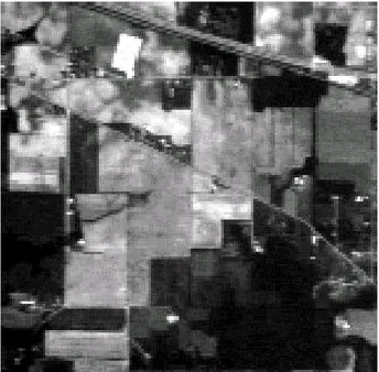
The considered data set referred to the agricultural area of Indian Pine in the northern part of Indiana (USA) [18]. Images were acquired by an Airborne Visible/Infrared Imaging Spectrometer (AVIRIS) in June 1992. The data set was composed of 220 spectral channels (spaced at about 10 nm) acquired in the 0.4-2.5
µ
m region. A scene 145x145 pixels in size was selected for our experiments (Figure 1 shows channel 12 of the sensor). The available ground truth covered almost all the scene. For our experiments, we considered the nine numerically most representative land-cover classes (see Table 1). The crop canopies were about a 5% cover, the rest being soil covered withthe residues of the previous year’s crops. No till, a minimum till, and a clean till were the three different levels of tillage, indicating a large, moderate, and small amount of residue, respectively [18].
Overall, 9345 pixels were selected to form a training set. Each pixel was characterized by the 220 features related to the channels of the sensor. All the features were normalized to the range from 0 to 1.
B. Results
Experiments were carried out to assess the performances of the proposed algorithms and to compare them with those of the SFS and SFFS algorithms in terms of both the solution quality and the computational load. SFS was selected for the comparison because it is well-known and widely used (thanks to its simplicity); SFFS was considered as it is very effective for the selection of features from large feature sets, and allows a good tradeoff between execution time and solution quality [5],[13].
As a criterion function, we adopted the average Jeffries-Matusita (JM) distance [4],[6],[7], as it is one of the best-known distance measures utilized by the remote sensing community for feature selection in multiclass problems:
h k hk c h c h k
JM
P
P
JM
∑∑
= >=
12
(9))
1
(
2
e
JM
b hk=
−
− hk (10)( )
(
)
+
+
−
+
=
−
−C k
C h
C
C
M
M
C
C
M
M
b
k h k h k h k h T hk2
ln
2
1
2
)
(
8
1
1 (11)the i-th class, bhk is the Bhattacharyya distance between the h-th and k-th classes, Mi and Ci are the mean vector and the covariance matrix of the i-th class, respectively. The
assumption of Gaussian class distributions was made in order to simplify the computation of the Bhattacharyya distance according to (11). As JM is a distance measure, the larger the obtained distance, the better the solution (in terms of class separability).
To better point out the differences in the performances of the above algorithms, we used the results of SFS as reference ones, that is, we plotted the values of the criterion function computed on the subsets provided by SA, FCS and SFFS, after dividing them by the corresponding values obtained by SFS (Fig. 2). For example, a value equal to 1 on the curve indicated as SFFS/SFS means that SFFS and SFS provided identical values of the JM distance. For the initializations of SA and FCS, we adopted the strategy of performing only one run, starting from the feature subset provided by SFS.
As can be observed from Figure 2, the use of SFFS and of the proposed SA and FCS algorithms resulted in some improvements over SFS for numbers of selected features below 20, whereas, for larger numbers of features, differences are negligible. The improvement obtained for 6 selected features is the most significant. Comparing the results of SA and FCS with those of SFFS on the considered data set, one can notice that the first two algorithms allowed greater improvements than the third (about two times greater, in many cases). Finally, a comparison between the two proposed algorithms shows that SA usually (but not always) provided better or equal results than/to those yielded by the FCS algorithm; however, differences are negligible (the related curves are almost completely overlapped in Fig.2).
In order to check if numbers of selected features smaller than 20 are sufficient to distinguish the different classes of the considered data set, we selected, as interesting
examples, the numbers 6, 9 and 17 (see Fig. 2). In order to assess the classification accuracy, the set of labeled samples was randomly subdivided into a training set and a test set, each containing approximately half the available samples. Under the hypothesis of Gaussian class distributions, the training set was used to estimate the mean vectors, the covariance matrices and the prior class probabilities; the Bayes rule for the minimum error [2] was applied to classify the test set. Overall classification accuracies equal to 78.6%, 81.4% and 85.3% were obtained for the feature subsets provided by the SA algorithm and numbers of selected features equal to 6, 9 and 17, respectively. The error matrix and the accuracy for each class in the case of 17 features are given in Table II. The inspection of the confusion matrix confirms that the most critical classes to separate are corn-no till, corn-min till, no till, min till and soybean-clean till; this situation was expected, as the spectral behaviors of such classes are quite similar. The above classification accuracies may be considered satisfactory or not, depending on the application requirements.
The other important characteristics to be compared are the computational loads of the selection algorithms, as not only the optimal search techniques, but also some sophisticated sub-optimal algorithms (e.g., generalized sequential methods [5]) exhibit good performances, though at the cost of long execution times.
For all the methods used in our experiments, the most time-consuming operations were the calculations of the inverse matrices and of the matrix determinants (the latter being required for the computation of the Jeffries-Matusita distance). Therefore, to reduce the number of operations to be performed, we adopted the method devised by Cholesky [19],[20]. In Fig.3, we give the execution times for SFS, SFFS, SA and FCS. All the experiments were performed on a SUN SPARC station 20.
proposed SA algorithm is the slowest. In the most interesting range of features (2 to 20), SFFS is faster even than the proposed FCS algorithm; it is slower for more than 25 selected features. In general, we can say that all the computations presented in Fig.3 are reasonable, as also the longest one (i.e. the selection of 50 out of 220 features by SA) took less than one hour. In the range 2 to 20 features, the SA algorithm took, on average, 5 times more than SFFS; the FCS algorithm took, on average, about 1.5 times more than SFFS. In particular, the selection of 20 features by the SA algorithm required about 3 minutes, i.e., 5.8 times more than SFFS; for the same task, FCS took about 1.6 times more than SFFS.
Finally, an experiment was carried out to assess, at least for the considered hyperspectral data set, how sensitive the SA algorithm is to the initial point, that is, if starting from random points involves a high risk of converging to local maxima associated with low-performance feature subsets. At the same time, this experiment allowed us to evaluate if adopting the solution provided by SFS as the starting point can be regarded as an effective initialization strategy. To this end, the number of features to be selected ranged from 1 to 20 out of the 220 available features. In each case, 100 different starting points were randomly generated to initialize the SA algorithm. The value of JM was computed for each of the 100 solutions; the minimum and the maximum of such JM values were determined, as well as the number of times the maximum occurred. For a comparative analysis, the minimum and maximum JM values are given in Fig.4 in the same way as in Fig.2, i.e., by using as reference values the corresponding JM values of the solutions provided by the SFS algorithm. In the same diagram, we show again the performances of the SFFS algorithm. As one can observe, with the 100 random initializations, even the worst performance (Min/SFS curve) can be considered good for all the numbers of selected features except 13 and 14. For these two numbers, considering only one random
starting point would be risky. To overcome this problem, one should run the SA algorithm a few times, starting from different random points. For example, with 5 or more random initializations, one would be very likely to obtain at least one good solution, even for 13 features to be selected. In fact, in our experiment, for 13 features to be selected, we obtained the maximum in 45 cases out of 100.
If one compares the diagram Min/SFS (Fig.4) with the SA/SFS one (Fig.2), one can deduce that the strategy that considers only the solution provided by the SFS algorithm represents a good tradeoff between limiting the computation time (by using only one starting point) and obtaining solutions of good quality. In particular, in only one case (four features to be selected), the solution obtained by this strategy was significantly worse than that reached by the strategy based on multiple random initializations. In addition, thanks to the way the SA algorithm operates, one can be sure that the final solution will be better than or equal to the starting point. Therefore, starting from the solution provided by SFS is certainly more reliable than starting from a single random point.
VI. D
ISCUSSION ANDC
ONCLUSIONSA new search strategy for feature selection from hyperspectral remote-sensing images has been proposed that is based on the representation of the problem solution by a discrete binary space and on the search for constrained local extremes of a criterion function in such a space. According to this strategy, an algorithm (SA) applying the concept of “steepest ascent” has been defined. In addition, a faster algorithm (FCS) has also been proposed that resembles the SA algorithn, but that makes only a prefixed number of attempts to improve the solution, no matter if a local extreme has been reached or not. The proposed SA and FCS algorithms have been evaluated and compared with the SFS and SFFS ones on a hyperspectral data set acquired by the
AVIRIS sensor (220 spectral bands). Experimental results have shown that, considering the most significant range of selected features (from 1 up to 20), the proposed methods provide better solutions (i.e. better feature subsets) than SFS and SFFS, though at the cost of an increase in execution times. However, in spite of this increase, the execution times of both proposed algorithms remain quite short, as compared with the overall time that may be required by the classification of a remote sensing image. For a comparison between the two proposed algorithms, we note that the FCS algorithm allows a better tradeoff between solution quality and execution time than the SA algorithm, as it is much faster and requires a deterministic execution time, whereas the solution qualities are almost identical. In comparison with SFFS, the FCS algorithm provides better solutions at the cost of an execution time that, on average, is about 1.5 times longer. For a larger number of selected features (more than 20), all the considered selection procedures provide solutions of similar qualities.
We have proposed two strategies for the initialization of the SA and FCS algorithms, that is, initialization with the results of SFS and initialization with multiple random feature subsets. Our experiments performed by the SA algorithm pointed out that the former strategy provides a better tradeoff between solution quality and computation time. However, the strategy based on multiple trials, which obviously takes a longer execution time, may yield better results. For the considered hyperspectral data set, when there was a significant difference of quality between the best and the worst solutions with 100 trials, the best solution was always obtained in a good share of the cases (at least 45 out of 100). Consequently, for this data set, the number of random initializations required would not be large (e.g., 5 different starting points would be enough).
According to the results obtained by the experiments, in our opinion, the proposed search strategy and the related algorithms represent a good alternative to the standard SFFS and
SFS methods for feature selection from hyperspectral data. In particular, different algorithms and different initialization strategies allow one to obtain different tradeoffs between the effectiveness of the selected feature subset and the required computation time; the choice should be driven by the constraints on the specific problem considered.
ACKNOWLEDGMENTS
The authors wish to thank Prof. D. Landgrebe of Purdue University (West Lafayette, Indiana, USA) for providing the AVIRIS data set and the related ground truth.
REFERENCES
[1] C. Lee and D.A. Landgrebe, “Analyzing high-dimensional multispectral data,”
IEEE Transactions on Geoscience and Remote Sensing, vol. 31, pp. 792-800, 1993.
[2] K. Fukunaga, Introduction to statistical pattern recognition. New York: Academic Press, 2nd edition, 1990.
[3] G.F.Hughes, “On the mean accuracy of statistical pattern recognizers,” IEEE Transactions on Information Theory, vol. IT-14, pp. 55-63, 1968.
[4] P.H. Swain and S.M. Davis, Remote sensing: the quantitative approach. New York:McGraw-Hill, 1978.
[5] A. Jain and D. Zongker, “Feature selection: evaluation, application, and small sample performance,” IEEE Transactions on Pattern Analysis and Machine Intelligence, vol. 19, pp. 153-158, 1997.
[6] L. Bruzzone, F. Roli, and S.B. Serpico, “An extension to multiclass cases of the Jeffreys-Matusita distance,” IEEE Transactions on Geoscience and Remote Sensing, vol. 33, pp. 1318-1321, 1995.
[7] L. Bruzzone and S.B. Serpico, “A tecnique for feature selection in multiclass cases,” International Journal of Remote Sensing, vol. 21, pp. 549-563, 2000.
[8] P.M. Narendra and K. Fukunaga, “A branch and bound algorithm for feature subset selection,” IEEE Transactions on Computers, vol. 31, pp. 917-922, 1977.
[9] J.Kittler, “Feature set search algorithm, “in C.H.Chen, Ed., Pattern Recognition and Signal Processing, Sijthoff and Noordhoff, Alphen aan den Rijn, Netherlands, 1978, pp.41-60.
Pattern Recognition, Coronado (CA), 1976, pp.71-75.
[11] E.Backer, and J.A.D.Schipper, “On the max-min approach for feature ordering and selection”, in The Seminar on Pattern Recognition, Liège University, Sart-Tilman, Belgium, p.2.4.1.
[12] P. Pudil, J. Novovicova, N. Choakjarernwanit and J. Kittler, “An analysis of the Max-Min approach to feature selection and ordering,” Pattern Recognition Letters, vol. 14, pp. 841-847, 1993.
[13] P. Pudil, J. Novovicova, and J. Kittler, “Floating search methods in feature selection,” Pattern Recognition Letters, vol. 15, pp. 1119-1125, 1994.
[14] M. Ichino, and J. Sklansky, “Optimum feature selection by zero-one integer programming,” IEEE Transactions on Systems, Man and Cybernetics, vol.14, pp. 737-746, 1984.
[15] W. Siedlecki and J Sklansky, “A note on genetic algorithms for large-scale feature selection,” Pattern Recognition Letters, vol. 10, pp. 335-347, 1989.
[16] F. Ferri, P. Pudil, M. Hatef, and J. Kittler, “Comparative Study of Techniques for Large Scale Feature Selection,” Pattern Recognition in Practice IV, E. Gelsema and L. Kanal , eds., pp. 403-413, Elsevier Science B.V., 1994.
[17] W. Siedlecki and J Sklansky,”On automatic feature selection,” Int. J. Of Pattern Recognition and Artificial Intelligence, vol.2, pp.197-220, 1988.
[18] P.F. Hsieh and D. Landgrebe, Classification of high dimensional data. Ph.D. Thesis, School of Electrical and Computer Engineering, Purdue University, West Lafayette, Indiana, TR-ECE 98-4, 1998.
[19] C.H. Chen and T.M. Tu, “Computation reduction of the maximum likelihood classifier using the Winograd identity,” Pattern Recognition, vol. 29, pp. 1213-1220, 1996.
[20] T.M. Tu, C.H. Chen, J.L. Wu, and C.I. Chang, “A fast two-stage classification method for high-dimensional remote-sensing data,” IEEE Transactions on Geoscience and Remote Sensing, vol. 36, pp. 182-191, 1998.
FIGURE AND TABLE CAPTIONS
Figure 1. Band 12 (wavelength range between about 0.51 and 0.52 [
µ
m]) of the hyperspectral image utilized in the experiments.Figure 2. Computed values of the criterion function for the feature subsets selected by the different search algorithms versus number of selected features. The values of the criterion function obtained by the proposed SA and FCS algorithms and by SFFS have been divided by the corresponding values provided by SFS.
Figure 3. Execution times required by the considered search algorithms versus number of selected features.
Figure 4. Performances of the SA algorithm with multiple random starts. The plot shows the minimum and maximum values of the criterion function obtained with 100 random starts versus number of selected features. For a comparison, the performances of SFS are used as reference values; the performances of SFFS are also given.
Table I. Land-cover classes and related numbers of pixels considered in the experiments.
Table II. Error matrix and class accuracies for the test-set classification based on the 17 features selected by the SA algorithm. Classes are listed in the same order as in Table I.
Figure 1 0,998 1 1,002 1,004 1,006 1,008 1,01 1,012 1,014 1,016 1 4 7 10 13 16 19 22 25 28 31 34 37 40 43 46 49 Number of features Ratio of JM distances SFFS/SFS SA/SFS FCS/SFS Figure 2
100 1.000 10.000 100.000 1.000.000 10.000.000 1 4 7 10 13 16 19 22 25 28 31 34 37 40 43 46 49 Number of features
Execution time (msec)
SFS SFFS SA FCS
0,996 0,998 1 1,002 1,004 1,006 1,008 1,01 1,012 1,014 1,016 1 3 5 7 9 11 13 15 17 19 Number of Features
Figure 4
ratio of JM distances 100 100 100 93 67 100 90 74 94 94 91 18 45 80 77 11 10 18 35 15Number of occurrencies of the Max
Max/SFS Min/SFS SFFS/SFS
TABLE I
Land-cover classes Number of training pixels C1. Corn-no till 1434 C2. Corn-min till 834 C3. Grass/Pasture 497 C4. Grass/Trees 747 C5. Hay-windrowed 489 C6. Soybean-no till 968 C7. Soybean-min till 2468 C8. Soybean-clean till 614 C9. Woods 1294 Overall 9345 TABLE II Ground Truth C1 C2 C3 C4 C5 C6 C7 C8 C9 Class Accuracy C1 584 9 0 4 0 24 65 6 0 84.4% C2 25 286 0 0 0 2 65 14 0 73.0% C3 0 0 223 4 0 0 5 4 1 94.1% C4 0 0 3 352 0 2 0 0 1 98.3% C5 0 0 0 0 253 0 0 0 0 100.0% C6 33 5 2 1 0 368 70 2 0 76.5% C7 99 44 10 1 0 58 949 62 0 77.6% C8 1 14 0 0 0 2 25 267 0 86.4% Classification C9 0 0 7 2 0 0 0 0 634 98.6%