A note on planar real Cremona transformations

-

-UNIVERSITAT DE BARCELONA

FACULTAT DE MATEMÁTIQUES

A NOTE ON PLANAR REAL

CREMONA TRANSFORMATIONS

A NOTE ON PLANAR REAL CREMONA TRANSFORHATIONS by

Jaume Llibre(*) and Carles Sim6(**)

(*) Secci6 de Matematiques, Facultat de Ciencies, Universitat Autonoma de Barcelona, Bellaterra, Barcelona, Spain.

(**) Facultat de Matematiques, Universitat de Barcelona, Barcelona, Spain.

Abstract. In th,U no.te we. p1tove. .tlta,t a polynomilll ma.pping T in .two

!te.al valtiabtu .6ueh .tlta,t i l i jaMbian i-6 eon-6.tan.t (.the. 60 eatte.d planM !te.al C1te.mona map-6I i-6 a b.i.je.dion be..twe.e.n R2 and R2. le..t IF,GI be. .the. polynomla.l eompone.n.t-6 06 T. We g.i.ve a complete global pic.tulte 06 .the 6amillf 06 cUltvU F = coM.tan.t and G = con-6.tan.t.

1 Introduction

The main purpose of this note is to prove the following theorem.

Theorem A. le..t F = F(~₁,x₂) and G = G(x₁,x₂

J

be .two 1te.al polynom.i.al-6 in .the .two !te.al valtiablu x

1,x2 .6Uch .tha.t i l i jacobian J = de..t(a(F,Gl/a(x1,x2

I I

i-6 a nonze1to con-6.tan.t. Then .the polynomilll ma.p ( F, G) : R2 - - R2 i-6 bijedive.

The key point in the proof of the injectivity of Theorem A is that the algebraic curves F(xl'x₂) = constant and G(x₁,x₂) constant are solutions of systems of ordinary differential equations of Hamiltonian type (with Hamiltonians F and G, of course). These systems have only a singularity of index two at the infinity point which consists of two elliptic sectors

For the proof of the onto character we analyze the Newton polygon of F and G. In order to make this analy~is easier we

p· note that using triangular maps of the type (x

1,x2)---+ (x1,x2+bx1), where b is a nonzero real number and p an integer such that p > 1, we obtain another Cremona map of the type

(1) where degree

F

< m and degree

G

< n. When F and G have the forro (1) the only possible diffeomorphic qualitative global pictures of the flow (for the Hamiltonians F or G) are given in Figure 1.a and Figure l.b (see section 2). In any case the global picture is homeomorphic to one of these two figures (see, again, section 2) where we have used the usual compactification of the plane adding one point p at infinity.

Figure 1 here

As a consequence of the onto character of T the flows with Hamiltonian F and G do not reach the infinity in finite time

(see section 3).

Remark l. The assumption that F and G are polynomials is necessary in Theorem A. The result is not true for analytical maps. For instance, if F(x₁,x₂)

=

-exp(x₂)cos(x₁exp(-2x₂)l and G(xl'x₂) = exp(x₂)sin(x

1exp(-2x2)) then J=l but the map

2 2

(F,G): R - - , . R is clearly not injective.

Remark 2. There is no restriction putting J = 1 because, if -1

J = a ,t. O, we can consider the map (a F ,G) instead of (F ,G).

Remark 3. A theorem similar to Theorem A for complex polynomials in two complex variables would prove the jacobian conjecture for two variables, that is, the inversemap is also polynomial (see [2],

[6J

and [7, Theorems 38 and

46] ).

In fact for the validity of the jacobian conjecture i t is enough to prove the injectivity. Remark 4. To prove the injectivity for a mapping T= (F,G):

c

2 - +

c

2, F and G complex polynomials with J= 1, we claim that it is enough to prove the injectivity for complex valued polynomials maps T' = (P,Q): R2 __..

c

2 in two real variables with J= 1. Suppose T

2

is not injective. Then there exist z,w E e such that Tz = Tw. Using translation, scaling and rotation we can assume that z and

w

are (0,0) and (1,0). Let T" be the map obtained from T by these changes of variables. The restriction of T" to R2 is of type T' and the claim is proved. Note thát T' is of type T' = (P

1 +iP2, Q₁ +iQ₂) where P₁, P₂,

o

1, Q2 are real valued polynomials. From Theorem A follows easely that if sorne of these four polynomials is identically zero T' is injective.

The authors would like to express their gratitude to Prof. P. Menal and Prof. C. Perell6 for his interest in the present work.

2 Proof of the injectivity

Let F and G be two polynomials in the hypotheses of Theorem A. This implies that the analytical Hamiltonian system XF given by

dx 1 3F F dt _{ax 2} x2 dx₂ 3F =-F dt ax X 1 1

has no critica! points. Of course F is a first integral of this system.

Lemma l. Fo1t ea.ch

IJ

E

r/

theJLe iA a un.ique Mlu.tlon

cj,)IJI

= _{(x 1} (.ti ,x 2(.tll 06 XF Ullth cp

0(yl = y de.6..úted on a rrr:tumal. open ..út.teJr.val (a,61

e

R 6uch .tha,t

llcf>.t(ylll-+<»

a6 .t + a olt .t + 6 wheJLe

11 11

deno.tu .the. EucUdea.n no!Un.

l.t iA poMi.ble a

= _, ,

6

=

+00 Olt bo.th.

For a proof of this lemma see [4,p.210].

Next we introduce the Poincar~ compactification far polynomial vector fields X(x) in the plane (see

[5)).

We consider in

R

3 the

-2 3 2 2 2

sphere S

=

{(x

1,x2,x3) E R x1 +x2+x3

=

1 and the plane

- 3

-P = {(x

1,x2,x3) E R : x3 1 }. For each point x of P of type -2

(x₁

,x

₂,1) we define the map f+:·P--+ S given by f+(x) =

2 2 1/2

(x

1,x2,1)/d(x) = (y1,y2,y3) = y where d(x) = (x1 +x2 +1) .

-

~

The image of P under f+ is the upper hemisphere H+ of S • Then f+ induces a field on H+: X(y) = Df+•X(x).

Let X= (P ,Q) a polynomial vector field on

P

of degree n = n-1

max (deg P , deg Q ) • Let r (y) = y

3 Then we claim that the field rX can be extended analytically to a vector field on H+

U

s

1

1 -2 where S = S

n

{y

3 = O} , the equator of the sphere.

In order to prove the claim (see [5] for details) we use five local carts (Ui ,cj,i) i=l,2,3, (Vi,lj,i) i=l,2 where

ui {y E

s2

: Y1 > O } ; _vi= {y E -2 S _{: Yi < O} } ;

cj,i

y

1 (yj,yk) j < k i ;,! j ,k; i

lj,i Y1 (yj,yk) 1 j < k i ;,! j ,k. Let y E

u

1nH+ and z=cp1(y). Then (z1,z2) = (y2,y3)/y1

=

(x2,1J/x1 . The vector field rX is expressed in the z coordinates as

n z2 ( -z lp ( 1 zl ) + Q( 1 zl ) -z₂P( 1 zl ) ) d(z)n-1

z ,

₂ z2

-

z2

,

z2

,

z/

z2 IQ

u

₂ we get n z2 ( P( zl 1 zl 1 n 1 z '

z

J -zlQ ( · ' -z ) d(z) - 2 2 z2 2

Furthermore the expressions of rX on

v

1,

v

2 are the ones of rX n-1

on

u

₁,

u

₂, respectively, multiplied by (-1) • In

u

3 the expression obtained is

It is easy to check that the different expressions of rX are analytical and compatible. Hence rX is extended to

"+

U

s

1 and

s1 is clearly invariant under the flow.

where Pj , Qj are homogenous polynomials of degree j. The field on

s

1 ('\

u

₁ ,

s

1 ('\

u

₂ is given by

respectively. In

s

1

nv

₁ ,

s

1

0

v

₂ we have the same expressions

times (-l)n-l.

On the other hand, let

s

2 be the sphere of R3 defined by

3 2 2 2 2

{ (yl'y

2 ,y3J E R : y1 + y2 + (y3 - 1/2) = 1/4 } . The plane R may be identified with the sphere

s

2 with the "north pole" p=(0,0,1) removed by means of the stereographic projection which assigns to each point

(x

₁

,x

₂) E R2 the point (y

1,y2,y3) E

s

2 through the relations x

1 = y1/(1-y3) , x2 = y2/(1-y3J,

' 2

where

If the degree of F, m, is greater than 2, this system is not defined at p, but i t can be extended by a change of the time scale. In any case we introduce a new variable u via

Then XF becomes dyl du dy2 du (2) 2

This system extends analytically the flow of XF from S - { p} to

s

2 (at least in a neighbohood of p). Note that the point p i s the unique critica! point of the new flow.

Lemma 2. In .the hypo.thuu 06 TheOJr.em A .the local phMe-p1w.tJi.lLlt 06 l>yl>.tem

(2)

Mound .the CJLUlcal poin.t p coM.Uü 06 .tJ.oo elüp.tic .sec.tou and .the Jr.u.t 6anl>

1

l>ee ~.p.219] 6°"- de6.ini.tionl>).

Proof. By the Poincar~-Hopf Index Theorem (see [3,p.366]) the index of p i s equal to two. Now we use the compactification of Poincar~. As we noted in section 1 we can always suppose that

F(x

1,x2) e x~

+

F(x1

,x

2), degF < m. Therefore P(x1

,x

2)

,.fx

2

,

m-1 Q(x

1,x2) = -mx1 - F _xl . The vector field (P,Q) on the parts of s1 which are in the carts

u

₁,

v

1,

u

2 and

v

2 (see Figure 2)

, m-1 m is given by R(z₁) = -m, R(z 1) = (..;1)· m, S(z1) = mz1 and m-2 lll S ( z 1) = ( -1 ) mz 1 , 2 2 { (yl,y2) E R : Y1 respectively. If we look at

s

1 as 2

+ Y2 1 }, then the only critica! points 1

are (0,1), (0,-1). We can visualize

"+

U

s as a closed disc bounded by

s

1. The flow on i t (recall that there are no critica! points inside and use Lemma 1) has the two qualitative possibilities given in Figure 3. When we glue the s1 into a point (and obtain

s

2) the respective pictures of Figure 3 become the ones given in Figure 1.a and l.b. This proves Lemma 2.

//

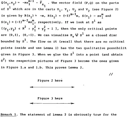
Figure 2 here

Figure 3 here

Remark l. The statement of Lemma 2 is obviously true for the analytical Hamiltonian system XG.

Remark 2. In the proof of Lemma 2 we strongly rely on the existence of the polynomial G such that the jacobian of (F,G) with respect to (x₁,x₂) is equal l. In fact for a general analytic Hamiltonian system XF without proper critica! points the stat~ ment is false. A counterexample is displayed by F(x

1,x2)=x2(x1x2-1) which has two hyperbolic sectors and four elliptic sectors at the infinity.

Lemma 3. (,l) The global 6low

06 XF

on

R

2

.l6 cli66eomOJtplúc, to the 6low g{ven

m

F{guJte

4.

(U) 16

the algebJuúe

euJtve F(x

₁

,x

₂

J = eow,ta.nt on

R2

,u: noneinpty₁ then

f t luu, only one eonneeted eomponent. Tlú6 eomponent .l6 cli66eomo1tplúe to R.

(ilil FoJt al! i e

R2 the cú'.gebJuúe

etlflve F(x)

=

F{i)

and the .tJto..jeetoJtq

<Pt(i) 06

XF

1tep1tuent the

~ame eWtve

in R2•

Proof. (i) follows from Figure 3.

(ii) The curves F(x)

=

constant on R2 have only one connected component. Otherwise, between two curves with the same value of F there would be a curve where F is a extremum and hence i t would be composed of critical points.

(iii) follows immediately from the Hamiltonian character and {ii).

Figure 4 here

Proof of the injectiviti of T. Let .pt and ljlt be the flows of XF and XG, respectively. Since the jacobian is 1 we have that

d

(G•.pt) {G•<Pt F} -1

dt

,

d (F•ljlt) = {Feljlt G} 1 dt

where { , } denotes the Poisson bracket {for more details see [1,p.193] ) • Then for each point

x

e R2 we have that

G(<Pt (x)) F(,j,t (x)) -t+G(x) t + F(i) (3) //

From (2) and Lemma 3 i t follows that the curves F(x) = constant

and G(x) constant have at most one point in common. So the

2 2

polynomial map (F,G) : R - R is injective.

//

8

3 Proof of the exhaustivity

It is not excluded up to now that for ~t or wt sorne point of R2 reaches the infinity in·finite time.

By

Lemma 3 (ii) the image of"R2 under F is an interval I ·of R.· There are· three possibilities: I is bounded, I is bounded from one side or I = R. If I is bounded from above, for each point x e: R2 i t follows from (2) that there is sorne time tco (x) < +co such that wt (xl goes to infinity when t

t

t co(x). In a similar way if I is bounded from below there is sorne time t _co (x) > -co such that wt<x> goes to infinity when t . t_co (x). These values tco (x), t_co (x) are the values a and B of Lemma l. Let us show that is exhaustive, that is, I

=

R (and therefore if follows that the orbits of XG reach the infinity only for unbounded time). The same will be true for G.

F

We suppose again F(x₁,x₂) = x~ + LFj(x₁,x₂). We consider j<m

the Newton polygon of F for the neighborhood of the infinity, i.e., the outer part of the boundary of the convex closure of the set { (r, s) E: N x N : F (x₁ ,x₂) =

~

ªrsx~x; with ªrs

t-

O } , see Figure 5. We claim that if there is sorne vertex (i,j) in the Newton polygon with one odd coordinate then F is exhaustive. We set x

2

=

xt/q, q odd, where -q/p belongs to the interval J whose extrema are the slopes of the sides of the polygon whích meet in (i,j) (eventually p i s negative if these two slopes are positive or one is positive and the other zero). Suppose i , j odd. Then we

F(x x = xp/ql 1' 2 1

select p even and for lx₁1 large we have ªijx1qi+pj)/q(1 +o(l)) with qi+pj odd. Therefore F is exhaustive. If i odd, j even, take any p such

that p/q E J and again F is exhaustive. Finally, for i even, j odd i t is enough to take p odd. Hence we can SUP,pose that all the verteces have even coordinates. If the coefficients associated to the verteces change the sign we have exhaustivity. We suppose for definiteness that all these coefficients are positive.

Figure 5 here

Let us take a side of the Newton polygon. The involved terms are of the type Fs =

f._

akxi+kpx~-kq where r is even

k=O

and g.c.d. (p,q) = l. These terms are dominant when x

2 = axl/q (or when x

1 =c=constant, if q=0). On this curve Fs(x1,x2) =

x¡qi+pj)/qajfr(b) where fr(b) = * ª k b k , b=a-q (or Fs(xl'x

2)

x~cjfr(b) , b=cp if q=0) and F(x

1,x2) = Fs(x1,x2)(1+o(l)) when (x

1,x2) + w if Fs(x1,x2) is unbounded on this curve.

If fr(b) has sorne real zero

b

of odd multiplicity, then in any neighborhood of

b

there are points b_, b+ such that fr(b_) < O, fr(b+) > O and hence F is exhaustive.

Let us suppose that all the real zeros of fr(b)_are of even (greater than zero) multiplicity. Then we consider the terms in the highest line parallel to the side through one of the points in the Newton diagram and let f(l) be the related

r

polynomial in b. If for one of the zeros b* of fr we have f(l) (b*) < O, we have done. For the case f(l) (b*) > O see later.

r r

If f{l) (b*) =O we continue the process with other lines parallel r

to the selected side, obtaining

t;

21 ,

first index such that f(t) (b*) _r

-1

O _. If

10

f(J) _{r ,} etc. Let t be the f(t) (b*) < O the exhaustivity

is clear. If for all t f (t) (b*)

=

O then we have that xq - axp

' r ' 2 1

is a factor of F (or XjX~P -a if p=O). Therefore F(x

1,x2)

_<x1-axi)F(x

1,x2)

+

C, where C is a constant. Then for the· Hamiltonian field we get F = apxl-l - (x¿ - ax1)F

xl xl

F = qx«r 1

f

+ (xq

2 - axP1¡ F . First we suppose p > O, q

t-

O. Then

x2 x2

p > 1 and we have a critical point at the origin if q > 1, which is an absurdity. Therefore F(xl'x₂) = (x₂ - ax1)F

+

C. Then the algebraic curve F = C has the real cornponents x₂ - axl = O,

F

= O. If F = O has real points in the curve x

2 - axi =O, then these points will be critica! points and this is impossible. If F

=

O has real points outside x₂-axi =O, we have a contradiction with Lemma 3 (ii). If F = O has no real cornponents then F(O ,x

2)

is a polynomial of even degree and thereforeF(O,x

2) is of odd degree, showing exhaustivity. A similar reasoning applies to the cases p < O and q = O.

If for all the sides of the Newton polygon we have no zeros of the related fr(b) polynornials or if the zeros being even there is sorne t such that f~t) (b*) > O for a zero b* of fr then F is positive definite for large values of ll<x

1,x2) 11 • Therefore the curve F(x

1,x2) = K is closed for K large enough. This implies that this curve is a periodic orbit for XF showing the existence of a critical point inside (see (4,p.254]) and therefore leading toan absurdity. This ends the proof that F is exhaustive. The sarne is true for G. Figure 5 displays the dorninant terms in the Newton polygon near infinity. If there are no terrns with exponents

(i,j), i < r but there is sorne point (r,s) with nonzero coefficient the Newton polygon ends on the point (r,s) with the maximum

Proof of the exhaustivity of T. We know that t,he flows ,j,'t , Wt exist for all t without going to infinity in finite time. Let

(x₀,y₀) e: R2 be any point and (t₀,s

0) = T(x0,y0). Then select any point (t,s) in R2. From (2) i t follows that

4>

5

_o

_5• ijlt-t

_o

(x0,y0)

=

(x,y) with T(x,y)

=

(t,s). Hence T is

exhaustive.

//

References

l. R. Abraham and J .E. Marsden, Founda,Uoru, 06 Meduuúe1,, Benjamín/ Cumrnings, 1978.

2. B.L. Fridman, On a c.luvi.ae-tvuzation 06 polynomi.al endomo-'lphMm!i 06 C , 2 Izv. Akad. Nauk SSSR, Ser, Mat. 37 (1973), 319-328.

3. S. Lefschetz, V.i66e-'len:Ua.l. Equa,Uont,: Geome.tJúc. theO!ty, Interscience, 1957.

4. J. Sotomayor, U~oeA de equa~Óe-6 cü6e-'lenc.-i.a-U o-'lCÜYWJt,ÚU,, Pro jeto Euclides 11, Instituto de Matemática Pura e Aplicada, Rio de Janeiro, 1979.

5. J. Sotomayor, CU-'lvM de6.(n.idM po-'l equa~cfu cü6e-'lenc..i,UJ,

no plano,

In~ titutodeMatemática Pura e Aplicada, Rio de Janeiro, 1981. 6. A.G. Vitushkin, On polynomi.al t-'laM6o-'lmation 06 C11,

"Manifolds-Tokyo 1973" (Prodeedings of the International Conference on Manifolds and Related Topics in Topology), 415-417, Univ. of Tokyo Press, 1975.

7.

s.s.s.

Wang, Ajacob.lanc.-'l.iteJU.on6o"-~epMab.iUty,J. of Algebra 65

(1980),453-494.

Captions for the figures

Fig. l. Qualitative picture of the flow of XF on s~

Fig. 2. The four carts used for

s

1.

1 -2 Fig. 3. Qualitative picture of the flow of (1) in H+Us e S .Case

(a) m odd: case (b) m even.

Fig. 4. Qualitative picture of theflowof XF.

....

>, bll

....

r..

. _J.6

Dlpbslt Legal 8.: 4.222-1982 BAACELONA- 1982