Verifica e validazione preliminare sull'accoppiamento del codice di calcolo RELAP5-3D e il codice di fluidodinamica computazionale ANSYS CFX

(1)

(2)

CIRTEN

Consorzio Interuniversitario per la Ricerca TEcnologica Nucleare

Lavoro svolto in esecuzione dell’Attività LP2.c.1_e

AdP MSE-ENEA sulla Ricerca di Sistema Elettrico - Piano Annuale di Realizzazione 2014

Progetto B.3.1 “Sviluppo competenze scientifiche nel campo della sicurezza nucleare e collaborazione ai programmi internazionali per il nucleare di IV generazione”

UNIVERSITY OF PISA

S. PIERO A GRADO NUCLEAR RESEARCH GROUP

VERIFICA E VALIDAZIONE PRELIMINARE

SULL’ACCOPPIAMENTO DEL CODICE DI CALCOLO

RELAP5-3D E IL CODICE DI FLUIDODINAMICA

COMPUTAZIONALE ANSYS CFX

Autori

F. Moretti

L. Mengali

F. Terzuoli

F. D’Auria

CERSE-UNIPI RL 1512/2015

Rev.0

PISA, 18 Settembre 2015

(3)

List of Contents

List of Contents ____________________________________________________ 2

List of Figures and Tables ____________________________________________ 3

Abstract __________________________________________________________ 5

1 Introduction ___________________________________________________ 6

2 NACIE Tests Selected for the V&V Studies____________________________ 7

2.1 Test #201 ____________________________________________________________ 8

2.2 Test #301 ___________________________________________________________ 11

2.3 Test #303 ___________________________________________________________ 13

3 RELAP5 Standalone Results ______________________________________ 16

3.1 RELAP5 Nodalization and Input Setup ____________________________________ 16

3.2 Test #201 RELAP-Standalone Results _____________________________________ 18

3.3 Test #301 RELAP-Standalone Results _____________________________________ 20

3.4 Test #303 RELAP-Standalone Results _____________________________________ 22

4 Coupled Code Results ___________________________________________ 24

4.1 New CFD Model ______________________________________________________ 24

4.2 CFD-RELAP Data Transfer Interfaces ______________________________________ 25

4.3 Test #201 Coupled Simulation Results ____________________________________ 27

4.4 Test #301 Coupled Simulation Results ____________________________________ 28

4.5 Test #303 Coupled Simulation Results ____________________________________ 30

5 Coupling Tool Improvements _____________________________________ 33

5.1 Parallelization _______________________________________________________ 33

5.2 Restart & Plot Files Manager ___________________________________________ 34

6 Conclusions ___________________________________________________ 37

(4)

List of Figures and Tables

Figure 1: Sketch (left) and 3D model (right) of NACIE loop (Ref. [5]). ... 7

Figure 2: Test #201 – Fuel pin simulator power ... 9

Figure 3: Test #201 – LBE flow rate (WARNING: unreliable measurement!) ... 9

Figure 4: Test #201 – LBE temperatures... 10

Figure 5: Test #201 – Water flow rate through the HX ... 10

Figure 6: Test #201 – Water temperatures at HX inlet and outlet ... 11

Figure 8: Test #301 – LBE temperatures... 12

Figure 10: Test #301 – Water flow rate and temperatures ... 13

Figure 12: Test #303 – Argon injection flow rate ... 14

Figure 13: Test #303 – LBE temperatures across FPS and HX ... 14

Figure 15: Test #303 – Water Temperature and flow rate ... 15

Figure 16: Sketch of RELAP5 nodalization ... 17

Figure 17: RELAP standalone results for test #201 – Power ... 18

Figure 18: RELAP standalone results for test #201 – LBE flow rate... 19

Figure 19: RELAP standalone results for test #201 – LBE temperatures ... 19

Figure 20: RELAP standalone results for test #201 – Water temperatures ... 20

Figure 27: CFD mesh: overall (a); bottom detail (b); top detail (c) ... 25

Figure 28: Sketch of CFD computational domain (a); coupling-adapted RELAP nodalization (b) ... 26

Figure 29: Interfaces for data transfer between CFX and RELAP ... 26

Figure 30: Test #201 Coupled Simulation Results – LBE flow rate ... 27

Figure 31: Test #201 Coupled Simulation Results – LBE temperature ... 28

Figure 32: Test #201 Coupled Simulation Results – Water temperature ... 28

Figure 34 Test #301 Coupled Simulation Results – LBE temperatures ... 29

Figure 35: Test #301 Coupled Simulation Results – Water temperature ... 30

Figure 37: Test #303 Coupled Simulation Results – LBE temperature ... 31

(5)

Figure 39: CFX Coupling Routines ... 34

Figure 40: Outer Coupling – Junction Box Calling Points ... 35

Figure 41: Inner Coupling – Junction Box Calling Points ... 36

Table 1: Variables exchanged from RELAP to CFX ... 27

(6)

Abstract

This report describes the work performed by the Gruppo di Ricerca Nucleare di San Piero a Grado (GRNSPG) of the University of Pisa (member of CIRTEN consortium) in the frame of the “Accordo di Programma MSE-ENEA sulla Ricerca di Sistema Elettrico - Piano Annuale di Realizzazione 2014”, particularly Project B.3.1, Task LP2.c.1_e. Aim of the work was to further improve and qualify a software interface that allows performing CFD-system code simulations, which had been developed by the same working group during previous PARs. Namely, the coupling tool was parallelized, so as to dramatically improve the cost-effectiveness of the coupled simulations compared to “serial” runs, and further Verification and Validation work was carried out by the simulation of experimental tests dealing with natural and assisted circulation of liquid metals in closed loops.

(7)

1 Introduction

This report describes the work performed by the Gruppo di Ricerca Nucleare di San Piero a Grado (GRNSPG) of the University of Pisa (as member of CIRTEN consortium) in the frame of the “Accordo di Programma MSE-ENEA sulla Ricerca di Sistema Elettrico - Piano Annuale di Realizzazione 2014” (Ref. [1]).

In particular, this report constitutes the deliverable LP2.c.1_e of the corresponding activity scheduled in “Linea Progettuale 2” of Project B.3.1.

The objective of the performed activity was to further contribute to the qualification and improvement of the CFD/system-code coupling tool that had previously been developed in the framework of PAR 2011, 2012 and 2013 by the same working group (Refs. [2], [3] and [4]).

As stated in the previous report, “the scientific and technological relevance of such contribution relies on the fact that the availability of qualified thermal-hydraulic analysis tools and methodologies, which combine multi-scale simulation capabilities, allows a more accurate analysis of nuclear reactor cooling systems (to support both design and safety assessment) in those cases featuring a close interaction between system-scale phenomena (e.g. the natural circulation in a nuclear reactor cooling loop) and local and inherently three-dimensional phenomena (e.g. the heat transfer between coolant and fuel rods, etc.)” The developed “coupling tool” consists of a software interface, implemented with a Graphical User Interface (GUI), which allows coupling

• the thermal-hydraulic system code RELAP5-3D v.4.1.3 (in short: RELAP), and • the CFD code ANSYS CFX v15.0 (in short: CFX).

Specific objectives of the present activity are:

1. To improve the coupling tool by extending its applicability to the parallel simulation (as far as the CFD part is concerned)

• The previously developed coupling tool was capable of running in “serial mode” only, i.e. without taking advantage of the parallel run capabilities of the CFD code. The limitation relied in the way the user-defined routines that handle the data communication to and from the CFD code had been coded. It then turned out that a further development effort was necessary to “parallelize” the tool.

• The parallelization obviously concerns the CFD part only, as the system code runs normally exhibit far smaller computational costs than CFD runs and their parallelization would not bring any appreciable benefits.

2. To extend the Verification & Validation (V&V) basis for the coupling tool through the simulation of experimental tests (and comparison of numerical results against measured data)

• For such purpose reference was made to one of the experiments that had been performed in the past on the NACIE test facility (ENEA-Brasimone) in the framework of an experimental campaign on natural and/or assisted circulation of a lead-bismuth eutectic alloy in a closed loop (the natural circulation being driven by an electrically heated fuel pin simulator and the assisted circulation being induced by Argon gas injection).

Both the above objectives were successfully achieved. Namely: the results from coupled simulations provided consistent results with the standalone system code simulations (Section 4); the parallelization was implemented and “validated”, in addition to further improvements to the coupling tool (Section 5).

(8)

2 NACIE Tests Selected for the V&V Studies

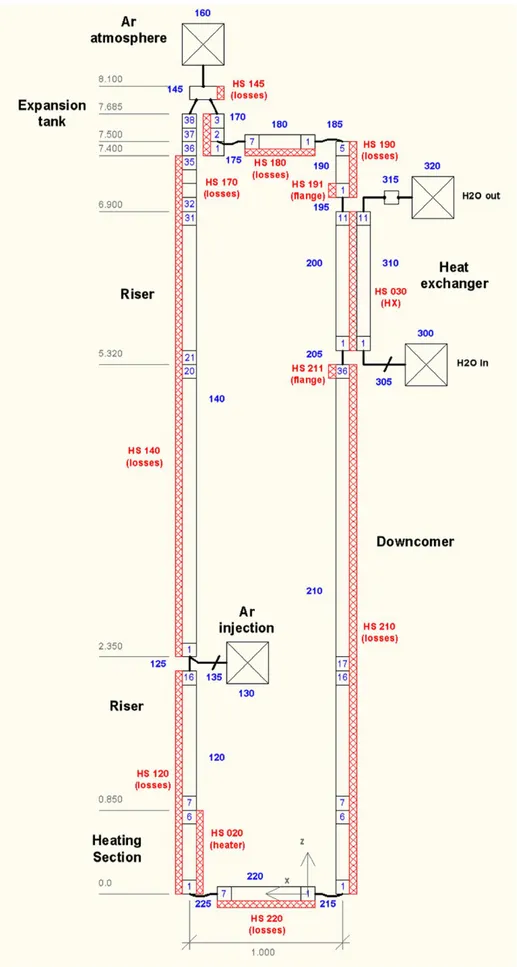
To support the V&V studies, reference was again made to experimental tests performed in 2012 on the NACIE test facility (ENEA-Brasimone), a description of which is available in Ref. [5] and, more synthetically, in the report of the activity performed during PAR2013 (Ref. [4]). Figure 1 is placed hereafter to remind of the NACIE configuration, and no further description is provided.

Figure 1: Sketch (left) and 3D model (right) of NACIE loop (Ref. [5]).

In particular, the following tests were considered (see Table 1 in Ref. [4]):

 #301 – Natural Circulation, 100% fuel pin simulator power (21.5 kW), no gas lift, heat sink available o NOTE: this test was uses also during PAR2013 activity; it has been referred to again here

following improvements in the RELAP5 nodalization.

 #303 – Natural + Assisted Circulation, 100% fuel pin simulator power (21.5 kW), 5 Nl/min gas lift, heat sink available

(9)

 #201 – Natural Circulation, 50% fuel pin simulator power (21.5 kW), no gas lift, heat sink available o NOTE: although the power is rated as 50 %, the test was conducted in three steps, the first

two of which featured a 100% power. Reference has been made here to the first step, so the simulated transient is similar to test #301.

Test #301 was described in Ref. [4]. However, for the sake of clearness, a short description of the three tests is provided hereafter.

2.1 Test #201

Figure 2 shows the power supplied to the fuel pin simulator (FPS) during the test. Three test phases are recognized, two at 100% and one at 50% power.

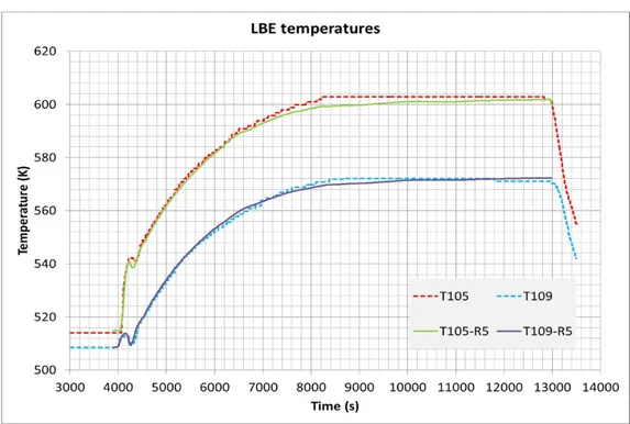
LBE flow rate measured during the experiment is plotted in Figure 3; however, such measurement is known to be unreliable for relatively small flow rates (< 10 kg/s), therefore such data cannot be used for any quantitative analysis. This consideration applies to all tests of the same experimental campaign (Ref. [5]). Figure 4 shows the trends of the LBE temperature measurements at the following four key locations:

• T103: inlet of heat exchanger (HX) • T104: outlet HX

• T105: a few meters downstream of the FPS • T109: T105: a few meters upstream of the FPS

During the 100%-power phases the temperatures stabilize after rising for about one hour. During the 50%-power phase the plateaus are reached more slowly and a much lower temperature level.

The differences T103-T104 and T105-T109 are similar (in the order of 30 K) but not coincident because of the heat losses of the loop in the section between T105 and T103, and between T104 and T109. The average LBE temperature during the first stationary phase is about 588 K.

It can be noticed that the initial LBE temperature ranges between 508 and 516 K. Detailed information on the temperature distribution along the loop, however, is unavailable.

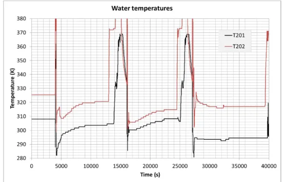
Figure 5 shows the measured water flow rate through the HX as well as the pump speed (during the first phase only), while the water temperature measured at the inlet and at the outlet of the HX are plotted in Figure 6.

The presented data seems to be affected by some inconsistencies, either due to systematic error measurements or to scarce information about the experimental setup, as explained hereafter.

Let us consider the stationary phase during the first 100%-power test. As no reliable LBE flow rate measurement is available, an estimate can be obtained through thermal balance between locations T109 and T105 (Qfps = Glbe T cp). If the heat losses are neglected, then one gets Glbe = 4.9 kg/s. Hence, the HX transferred power can be estimated as about 20.7 kW. On the other hand, based on flow rate and temperature measurements on the HX secondary side, one would obtain 17.4 kW. Such discrepancy seems to suggest that the water flow rate data is not correct (but other sources of error may exist).

Moreover, it known from ENEA experimentalists that the HX water admission valve was manually operated during the test, and that vapour formation occurred at the beginning, but no detailed data is available to characterize such phase of the test. Furthermore, accurate data is unavailable also about HX materials (especially the steel powder) and thermal insulating material. In general, such lack of detailed information and accurately measured data makes it difficult to setup accurate simulation models, and requires considerable “tuning” efforts to obtain results that can reasonably match the available measured data. Such limitation has heavily affected the conduction of the activity.

(10)

Figure 2: Test #201 – Fuel pin simulator power

(11)

Figure 4: Test #201 – LBE temperatures

(12)

Figure 6: Test #201 – Water temperatures at HX inlet and outlet

2.2 Test #301

This test (see Figure 7 to Figure 10) is similar to the 100%-power phases of the test #201 described above. The main difference is represented by the initial temperature, which is in the range 552 to 563 K, i.e. about 50 K higher than in test #201. Consequently, higher temperature levels are reached during the transient before the temperatures again (almost) stabilize at values close to those of test #201.

The same considerations about lack of information apply here as for test #201.

A further complication (or “degree of freedom” in modelling) is represented by the water flow rate showing a stepwise decrease at about 22000 s, which obviously yields an outlet water temperature increase.

(13)

Figure 8: Test #301 – LBE temperatures

(14)

Figure 10: Test #301 – Water flow rate and temperatures

2.3 Test #303

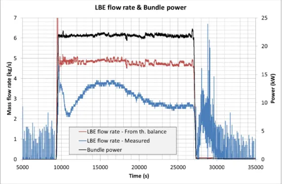
This test, in addition to the power supplied by the FPS, features an injection of Argon into the riser pipe downstream of the FPS, aimed at further enhancing the flow. Figure 11 to Figure 15 show the relevant measured quantities.

During the first phase of the test, both FPS power and gas injection are present. The LBE temperatures rise until they reach a maximum, then they decrease and tend to stabilize. At about 21000 s the Ar injection is disabled, and this causes an abrupt decrease in the flow rate (to less than one half) and hence an increase in the LBE temperature difference across the FPS (and across the HX). Then the temperatures rise again and tend to stabilized to a higher level than before.

(15)

Figure 12: Test #303 – Argon injection flow rate

(16)

Figure 14: Test #303 – LBE flow rate (WARNING: unreliable measurement!)

(17)

3 RELAP5 Standalone Results

3.1 RELAP5 Nodalization and Input Setup

A sketch of the RELAP5-3D nodalization used for all standalone simulations is shown in Figure 16. It is basically the same as that used in the former activities (Ref. [4]), although it includes several improvements and corrections. A few explanatory comments are added hereafter:

 The Argon injection is handled by the time-dependent volume 130 and the time-dependent junction 135, which are obviously not used for the natural-circulation-only tests.

 The heat structure #10 (not shown in the figure) accounts for the non-heated parts of the fuel pin simulator bundle (i.e. dummy rod and support rods).

 The heat structure #20 represents the heated pin (i.e. it provides the FPS power).

 The heat structure #30 represents the HX; more precisely, it accounts for the heat transfer between LBE and water. Its modelling is critical because the thermal-hydraulic behavior of the system is very much sensitive to the HX heat transfer coefficient (HTC), which in turn depends on the LBE-steel convective transfer, the water-steel convective transfer, and the conductive transfer through the steel pipes and the steel powder contained within (see HX description in Ref. [5]). The heat conduction coefficient is the most sensitive parameter, and is known to have values in the range 8 to 12. This is a rather important source of uncertainty, and “tuning” is needed to setup a simulation input that matches the measured quantities.

 All the other heat structures handle the heat losses. Again, insufficient information on the thermal insulation is available, therefore reasonable starting assumptions (on insulating material thickness, density, heat conduction coefficient and heat capacity) have been made, which have then been “tuned”.

 The above heat structures that model heat losses have been also used to implement the cable heating power.

 Additional heat structures have been implemented to model the HX flanges (with their thermal capacity).

 Key locations for post processing are: o Node 14 of pipe 140 for T105 o Node 9 of pipe 210 for T109

o Single junction 125 for LBE mass flow rate o Branch 315 for water temperature at HX outlet

 Based on the available geometric information and on the assumption that the heat losses are uniformly distributed along the loop, one can estimate that the heat losses occurring between the locations of T109 and T105 are about 38% of the total heat losses. Such estimate is relevant to power balance considerations.

o E.g. the temperature increase between T109 and T105 is due to the net power supplied to the LBE, which results from the FPS power minus the heat losses in that section.

 Another critical modelling issue is represented by the HX secondary side, as regards the steel-to-water convective heat transfer. In fact, it is known that at the beginning of the test the valve admitting the water to the HX was operated manually, until relatively stable conditions were achieved. Such initial phase was characterized by vapour formation and complex (“chaotic”, in a sense) heat transfer conditions. The available set of experimental information is not sufficient to

(18)

support an accurate modelling; therefore it was necessary to resort to simplifying assumptions and parameter calibration.

(19)

3.2 Test #201 RELAP-Standalone Results

The simulation of this test was set up with the following modelling options and assumptions:

 Total power losses = 2 kW (derived from power balance considerations during the quasi-stationary phase)

 Tuned parameters:

o FPS grid spacer pressure loss coefficients

o HTC for insulation-air convective transfer (air temperature being arbitrarily set to 10 °C) o Thermal conductivity of HX steel powder

o Thermal conductivity of mineral wool o Heating cables power (before FPS power on) o HTC for convective transfer between water and HX

 As explained above, the set of TH information concerning the water flow on the HX secondary side is inconsistent with the thermal balance considerations on the LBE side. The assumption was then made that the water flow rate measurement is incorrect and that the actual flow rate is that obtained from thermal balance (which yields a value 15% larger than the “measured” one). After many different attempts, this turned out to be the only modelling approach through which satisfactory results could be obtained.

The results of the reference simulation (obtained after a rather long calibration process) are shown in the following figures.

The HX power and the lost power are plotted in Figure 17 along with the FPS power (imposed as a boundary condition). During the first 4000 s the HX is not balancing the FPS and the lost power, which means that the internal energy of the system is increasing: this is evident in the temperature trends, which show a general increase during that period.

(20)

The resulting flow rate is shown in Figure 18, along with the measured trend as well as that obtained from thermal balance considerations (that is appropriate only during the stationary phase, since the unsteady terms were not accounted for in such balance). As already explained the measured flow rate is unreliable and must not be considered.

As regards the LBE temperatures, rather satisfactory results are shown in Figure 19.

Finally, water temperatures are plotted in Figure 20; apart from the initial (practically unavoidable) discrepancies, the calculated outlet temperature matches the measured trend, as a result of having imposed a balance-consistent water flow rate instead of the measured one.

Figure 18: RELAP standalone results for test #201 – LBE flow rate

(21)

Figure 20: RELAP standalone results for test #201 – Water temperatures

3.3 Test #301 RELAP-Standalone Results

The simulation of this test was performed before that of test #201, was based on a slightly different modelling approach and did not benefit from some improvements and optimization that were introduced in the nodalization later on.

In particular, the inaccurate HX secondary side modelling resulted in HX power being highly over-predicted during the initial phase of the transient. In order to compensate for that, the heating cables power was fictitiously prolonged beyond the start of the FPS power and then ramped down to zero in about 5000 s. This allowed adjusting the overall power balance and obtaining reasonable results in terms of temperatures.

The calculated LBE mass flow rate is plotted in Figure 21, along with the trend estimated through a thermal balance. Contrary to test #201, in this case the balance did not account for the heat losses; therefore the reference flow rate is somewhat over-predicted; however, the error is estimated to be in the order of a few % only.

Figure 22 shows the results in terms of LBE temperatures, which overall exhibit a satisfactory behavior. There is some margin for further improvement, which would require additional parameter tuning. That is not necessary for the present coupling-validation purposes.

The water temperature at the outlet of the HX is plotted in Figure 23. The same considerations as above apply.

(22)

Figure 21: RELAP standalone results for test #201 – LBE flow rate

(23)

Figure 23: RELAP standalone results for test #201 – Water temperatures

3.4 Test #303 RELAP-Standalone Results

Such as for test #301, also the simulation of this test was performed before that of test #201, using a less optimized modelling.

The calculated LBE flow rate is shown in Figure 24, where it is compared against the flow rate obtained from thermal balance as well as the measured one (which, again, is to be considered as unreliable).

The LBE temperature trends are plotted in Figure 25. The general trends are satisfactory, both from the qualitative and the quantitative point of view.

(24)

Figure 26 show the water temperature trends. The temperature at the HX outlet is slightly over-predicted during the final phase of the transient.

By improving the HX modelling one could improve the results during the temperature rise phase, and with further parameter calibration more accurate temperatures could be obtained for the NC-only phase (i.e. after 21000 s). The current results are, however, fully adequate for the present purposes.

Figure 25: RELAP standalone results for test #303 – LBE temperatures

(25)

4 Coupled Code Results

4.1 New CFD Model

A new CFD model was developed to perform the RELAP-CFX coupled simulations. Its main features are described hereafter (see also Figure 27):

 The overall computational domain is halved by exploiting the symmetry across the middle plane of the loop. This allows reducing the number of meshes and the computational effort.

 In addition to the fluid domain, also solid domains are included in order to simulate the heat conduction through the steel pipe and the insulating material, and the convective heat transfer between the LBE and the steel; in other words: Conjugate Heat Transfer (CHT) simulations are performed. Heating cables power is implemented here too.

 Likewise, the fuel pin simulator (heated pin, dummy pin, support bar) is modelled via coupled solid domains.

 The fluid domain includes:

o a short section of the bottom horizontal pipe that connects to the test section; in order to reduce the topological complexity of the entrance region and its impact in terms of mesh density and quality and related computational cost, the geometry of the entrance was modified into a rectangular section, with same flow area of the real pipe. Such modification is expected not to affect the quality of the simulation at all.

o riser pipe (until about 1.4 m above the bottom of the FPS)

 The mesh is fully hexahedral and relatively high quality. It counts about 143000 nodes (67600 in the fluid domain, and the rest in the various solid domains). Details are shown in Figure 27.

o The qualification of CFD results would certainly require mesh refinement and sensitivity analysis, along with the application of various other Best Practice Guidelines (Ref. [8]). However this is out of the scope and objectives of the present work, therefore obtaining a good-quality yet relatively coarse mesh has been the preferred approach, so as to be able to run relatively fast calculations.

 As regards the heat losses, the same characteristics as in the RELAP standalone model are implemented.

 The LBE thermo-physical properties have been implemented so as to be consistent with RELAP libraries.

 To avoid the need of very fine meshes, the spacer grids of the fuel pin simulator were not modelled explicitly. Therefore it was necessary to implement a momentum sink (i.e. a volumetric additional flow resistance term, which appears in the momentum balance equation) to account for their effect. The model resistance parameter was obtained through a rough calibration process.

(26)

(a)

(b)

(c) Figure 27: CFD mesh: overall (a); bottom detail (b); top detail (c)

4.2 CFD-RELAP Data Transfer Interfaces

As explained in previous reports (Refs. [3] and [4]), the adopted coupling approach is such that a part of the system code domain is “replaced” by the CFD model. This requires an appropriate handling of the interfaces between the two domains, in order to allow a proper exchange of variables.

From the point of view of the CFD domain, the things are apparently easy: as shown in Figure 28(a), the interfaces are represented by the “inlet” and “outlet” boundaries; in principle, any solved variable can be transferred through those boundaries (provided that adequate tools for the data communication are in place, e.g. User Fortran Routines).

From the RELAP point of view, several modifications in the nodalization and in the calculation input are necessary to make the coupled-calculation possible. As shown in Figure 28(b), parts of the standalone nodalization must be removed, while some new hydraulic components have to be introduced. Namely, the horizontal pipe 220 is connected to a time dependent volume (230) through a single junction (225); the fluid flow rate to be imposed at CFD inlet as a boundary condition is “read” at 225, while the pressure that has to travel back from the CFD inlet to the RELAP domain is input into the time-dependent volume. The

(27)

temperature to be fed into the CFD inlet can be read from the pipe 220. Likewise, the CFD outlet temperature is transferred to the pipe 120 and the flow velocity to the new time-dependent junction 115; on the other hand, the RELAP pressure at pipe 120 is transferred back to the CFD outlet.

Control variables need to be defined in RELAP in order to apply the boundary conditions that are “received” from CFX.

A detailed account of all the above items involved in the coupling is provided in Figure 29, Table 1 and Table 2. The task of handling the transfer of data through those interfaces is performed, under the supervision of the Coupling Master, by the User Fortran Routines (described in Refs. [2] to [4]; see also Section 5.1 about recent improvements).

It is worth noticing that the pressure transferred from CFX to RELAP is a “total pressure” (i.e. it includes the dynamic term), while the pressure transferred from RELAP to CFX is static. This required some modifications to the Fortran Routines.

Furthermore, since velocities are transferred instead of mass flow rates, it is necessary to correct the velocities so as to account for possible differences between CFX and RELAP connecting flow areas, in order to assure the mass conservation.

(a) (b)

Figure 28: Sketch of CFD computational domain (a); coupling-adapted RELAP nodalization (b)

(28)

Table 1: Variables exchanged from RELAP to CFX

Var # Variable From To

001 T 22005 inlet

002 V 22500 inlet

006 p 12001 outlet

Table 2: Variables exchanged from CFX to RELAP

Var # Variable From To Control var.

003 p (tot) inlet 23001 9001

004 T outlet 11001 9002

005 v outlet 11500 9003

4.3 Test #201 Coupled Simulation Results

The results of the RELAP/CFX coupled simulation of test #201 are shown in Figure 30 to Figure 32, and there compared against those of standalone RELAP simulations as well as the experimental trends.

The LBE mass flow rates predicted by the standalone and the coupled simulations are almost coincident; the very tiny difference (which is certainly acceptable in present context) can be explained by the pressure loss model implemented in the CFD calculation being not exactly equivalent to that of the RELAP simulation setup.

Likewise, the results of the two simulations are almost coincident also in terms of LBE temperatures at location T105 and T109. The same applies to the water temperature at the HX outlet.

In summary, the results of the RELAP/CFX coupled simulation are consistent with those of the standalone RELAP simulation. This provides evidence of the correct implementation and operation of the coupling tool.

(29)

Figure 31: Test #201 Coupled Simulation Results – LBE temperature

Figure 32: Test #201 Coupled Simulation Results – Water temperature

4.4 Test #301 Coupled Simulation Results

The results of the RELAP/CFX coupled simulation of test #301 (in terms of LBE flow rate, LBE temperatures and water temperature at HX outlet) are shown in Figure 33 to Figure 35, and there compared against those of standalone RELAP simulations as well as the experimental trends.

Like for test #201, the results of the two simulations are consistent and show that the coupling tool is correctly implemented and works as intended. Somewhat larger (than above) discrepancies appear in LBE temperature trends, which are explained by some differences in the insulating material properties

(30)

implemented in the CFD model with respect to those used in RELAP. Such difference has then been fixed in later simulations (e.g. of test #201).

While such discrepancy does not constitute an issue as to the demonstration of the proper performance of the coupling tool, it provides food for thought about the role of the “user effect” in coupled-code analyses and the related V&V issues: particularly, about the larger amount of modelling and numerical parameters that the analyst has to deal with, which in turn translates into a larger number of sources of error and uncertainties.

Figure 33: Test #301 Coupled Simulation Results – LBE flow rate

(31)

Figure 35: Test #301 Coupled Simulation Results – Water temperature

4.5 Test #303 Coupled Simulation Results

The results of the RELAP/CFX coupled simulation1 of test #303 (in terms of LBE flow rate, LBE temperatures and water temperature at HX outlet) are shown in Figure 36 to Figure 38, and there compared against those of standalone RELAP simulations as well as the experimental trends. In this case the agreement between standalone and coupled results is not satisfactory from the quantitative point of view, because the coupled code run predicted some 2% higher LBE flow rate, and slightly discrepant LBE temperature trends. Such discrepancies are not due to possible issues with the coupling scheme, rather they reveal some inconsistencies in the setups of the two simulations, which need to be identified and corrected. Hence, the results obtained for test #303 provide a somewhat less strong evidence of the good performance of the coupling tool in exam, compared to the previous tests. In other terms, it can be concluded that the developed RELAP/CFX coupling interface runs in a proper and consistent way as desired while, on the other hand, the setup of a coupled simulation requires special care (by the analyst) in defining consistent material properties and initial and boundary conditions over both computational domains.

1

(32)

Figure 36: Test #303 Coupled Simulation Results – LBE flow rate

(33)

(34)

5 Coupling Tool Improvements

5.1 Parallelization

Parallel computing is usually indispensable to speed-up CFD simulations with complex and highly refined meshes (high number of computational nodes). A new version of the coupling tool, suitable for parallelization, was then developed, thus allowing a broader range of applications.

In CFX, User Fortran Routines are running independently on each parallel node and are not meant to communicate across parallelization borders. To allow communication between the different “computing nodes” (aver which the parallel calculation is distributed) a specific shared memory area in the CFX Memory Management System was used and most of the previously developed User Fortran Routines had to be modified in order to allow data exchange with such dedicated memory area.

A short description of the modifications implemented for the developed User Fortran routines is given below, together with an updated sketch (Figure 39) illustrating their updated roles within the coupling strategy.

jcb_init: Junction Box Routine that initialises the coupled simulation. In particular, it creates all the required data areas for variables handling and initialises their values to the ones assigned by the user. Moreover it set initial parameters for synchronization management. It also creates the dedicated memory area accessible to all the parallel nodes.

jcb_exchange: New junction box routine substituting the jcb_read and jcb_write routines developed in previous works (Ref. [3]). It is called at the “User input” start of every coupled CFX step (either a new time-step for explicit coupling scheme, or a new inner iteration for the semi-implicit scheme). It manages the data exchange between the codes for the CFX sub-domain. On one hand, it takes the data calculated in the previous coupled step (stored in the shared memory area by the jcb_out routine) and writes coupling variables, time step size and other synchronization parameters to specific CFX result files to be sent to RELAP. On the other hand, it waits for permission from the Synchronization Manager to read RELAP result files from the previous coupled step. After the needed conversions (due to possible data inconsistencies), it writes the collected values in the shared memory area to be read by the cel_input routine.

cel_input: user CEL routine. It takes the variables stored in the shared memory area by the jcb_exchange routine and uses them to compute suitable boundary conditions.

jcb_out: junction box routine, called at the end of every coupled CFX step (either inner or outer loop). It computes (separately in each partition) suitable averages of the variables to be sent to RELAP and store them along with the time step size and other synchronization parameters in the dedicated data area accessible to all parallel nodes.

jcb_end: junction box routine. When ending conditions (either from the internal solution or from the Synchronization Manager) are identified, this routine stops the coupled simulation, ending the CFX simulation and sending a stop message to the Coupling Manager. Only minor changes required.

(35)

Figure 39: CFX Coupling Routines

Moreover, the calling points for the different Junction Box Routines had to be modified for the correct operation within parallel runs. The new calling points are shown in Figure 40 and Figure 41, for the explicit and semi-implicit coupling scheme respectively.

Concerning the V&V aspects, it was obviously necessary to check that the parallelization was correctly implemented and was performing as expected. To do that, the same coupled simulations that had been run in serial mode were repeated in parallel mode using the new coupling interface and distributing the CFD calculation over two parallel processes. The results obtained from the parallel runs are perfectly matching those obtained from the serial calculations, and this allows stating that the parallelization is validated.

5.2 Restart & Plot Files Manager

In order to avoid excessive dimensions of the RELAP restart and plot files the previous versions of the coupling tool used an external Visual Basic routine (CSES) developed at GRNSPG (Ref. [2]). Such a tool was developed specifically for RELAP5 and in some cases showed undesired behaviours if used with RELAP5-3D. To solve this issue a new routine was developed in PERL directly within the Coupling Master. Before the actual start of the coupled simulation, this new algorithm runs some test RELAP simulations using the provided input in order to identify some problem specific information about the restart and plot files. During the coupled simulation, the restart file is cut maintaining only the information required for the continuation of the coupled simulation. Similarly, the plot file is managed in order to avoid the unnecessary repetitions related to the numerous restarts required for the coupled simulation. It is important to underline that reasonable settings (e.g. max time steps, initialisation values, etc.) should be provided in the RELAP input in order to allow the first test simulation to run correctly.

(36)

(37)

(38)

6 Conclusions

The performed activity dealt with the improvement and the additional qualification (through V&V) of the RELAP5-3D/CFX coupling interface that had been developed during previous PARs, in order to substantially extend the range of its possible application to the analysis of nuclear reactor coolant systems, with particular reference – but not limited – to liquid metal-cooled reactors. The advantage in coupling a CFD code to a system code relies in allowing the predictive analysis of a complex thermal-hydraulic system (such as a large closed circuit with all of its active and passive components) by a 1D approach while, at the same time, focusing on the accurate description of the multi-dimensional turbulent flow and heat transfer processes occurring at a particular section or component of the system.

The qualification-related part of the work followed-up the work already started during the previous PAR, and consisted in applying the coupling tool to the simulation of a few tests performed on the NACIE test facility during an experimental campaign in 2012, involving the natural/assisted circulation of lead-bismuth eutectic. The results of the coupled-code simulations have been compared against those obtained from RELAP5 standalone simulations (the development of which has constituted a substantial part of the activity); the comparison showed consistency between the two sets of results, thus proving the correct implementation and effective operation of the coupling tool, and particularly its applicability to coolant systems involving natural circulation flows of liquid metals.

The improvement-related part of the work consisted in the parallelization of the coupling tool, i.e. in allowing the execution of a parallel CFX simulation coupled to a serial RELAP simulation. Owing to the large computational effort usually required by a CFD analysis (far larger than by a system code run), the parallel CFD calculation capability is of critical importance whenever dealing with problems of practical interest that involve non-trivial geometries and relatively complex fluid-dynamic phenomena. The parallelization of the coupling tool required a re-coding of the User Fortran Routines that handle the data exchange between the two codes. In addition, further improvements were implemented in the coupling master routine, in order to optimize the file and data management.

(39)

References

[1] ENEA e Ministero dello Sviluppo Economico, Accordo di Programma sulla Ricerca di Sistema Elettrico, Piano Annuale di Realizzazione (PAR) 2014, Gennaio 2015.

[2] L. Mengali, M. Lanfredini, F. Moretti, F. D’Auria, Stato dell’arte sull’accoppiamento fra codici di sistema e di fluidodinamica computazionale. Applicazione generale su sistemi a metallo liquido pesante, CIRTEN – Università di Pisa – Gruppo di Ricerca Nucleare di San Piero a Grado (GRNSPG), Report RdS/2012/1509, 31 Luglio 2012 – Versione 0, CERSE-UNIPI RL 1509/2011, Lavoro svolto in esecuzione dell’Attività LP3-C1.C AdP MSE-ENEA sulla Ricerca di Sistema Elettrico - PAR 2011.

[3] L. Mengali, M. Lanfredini, F. Moretti, F. D’Auria, Accoppiamento di codici CFD e codici di sistema, CIRTEN – Università di Pisa – Gruppo di Ricerca Nucleare di San Piero a Grado (GRNSPG), Report RdS/2013/048, 6 Settembre 2013 – Versione 0, CERSE-UNIPI RL 1510/2013, Lavoro svolto in esecuzione dell’Attività LP2-C1_d Progetto B.3.1 - AdP MSE-ENEA sulla Ricerca di Sistema Elettrico - PAR 2012.

[4] F. Moretti, M. Lanfredini, L. Mengali, F. D’Auria, Accoppiamento di codici CFD e codici di sistema, CIRTEN – Università di Pisa – Gruppo di Ricerca Nucleare di San Piero a Grado (GRNSPG), Report CERSE-UNIPI RL 1511/2014, 22 Settembre 2014 – Versione 0, Lavoro svolto in esecuzione dell’Attività LP2-C1_d Progetto B.3.1 - AdP MSE-ENEA sulla Ricerca di Sistema Elettrico - PAR 2013.

[5] M. Polidori, P. Meloni, NACIE Benchmark Specifications and Experimental Data (LACANES) - Task Guideline for Phase 3: Characterization of NACIE (draft)

[6] ANSYS CFX-15.0 User Manual, 2013 (embedded in the software package).

[7] Idaho National Laboratories, RELAP5-3D Code Manuals, Appendix A – RELAP5-3D Input Data Requirements (version 4.0), INEEL-EXT-98-00834-V2, March 2012 (downloadable from

http://www.inl.gov/relap5/r5manuals.htm)

[8] Mahaffy, J. ET AL., Best Practice Guidelines for the use of CFD in Nuclear Reactor Safety Applications, NEA/CSNI/R(2014)11, 2015