A New Shape Similarity Framework
for brain fibers classification
Ph.D. Thesis
July 9, 2018
Università degli Studi di Verona
Advisor:
Prof. Paolo Fiorini
Series N◦: TD-06-18
Università di Verona Dipartimento di Informatica Strada le Grazie 15, 37134 Verona Italy
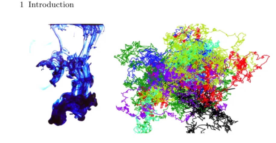
Goethe-Diffusion Magnetic Resonance Imaging (dMRI) techniques provide a non-invasive way to explore organization and integrity of the white matter structures in hu-man brain. dMRI quantifies in each voxel, the diffusion process of water molecules which are mechanically constrained in their motion by the axons of the neurons. This technique can be used in surgical planning and in the study of anatomical connectivity, brain changes and mental disorders. From dMRI data, white matter fiber tracts can be reconstructed using a class of technique called tractography. The dataset derived by tractography is composed by a large number of stream-lines, which are sequences of points in 3D space. To simplify the visualization and analysis of white matter fiber tracts obtained from tracking algorithms, it is often necessary to group them into larger clusters or bundles. This step is called clus-tering. In order to perform clustering, a mathematical definition of fiber similarity (or more commonly a fiber distance) must be specified. On the basis of this met-ric, pairwise fiber distance can be computed and used as input for a clustering algorithm. The most common metrics used for distance measure are able to cap-ture only the local relationship between streamlines but not the global struccap-ture of the fiber. The global structure refers to the variability of the shape. Together, local and global information, can define a better metric of similarity. We have extracted the global information using a mathematical representation based on the study of the tract with Frénet equations. In particular, we have defined some intrinsic parameters of the fibers that led to a classification of the tracts based on global geometrical characteristics. Using these parameters, a new distance metric for fiber similarity has been developed. For the evaluation of the goodness of the new metric, indices were used for a qualitative study of the results.
Acknowledgments
A sincere and esteemed thanks to Prof. Paolo Fiorini, not only for giving me the opportunity to undertake this path, but also for all that he has taught me on a human level. As he repeated to me several times: "The doctorate is a gym of life". And with so much training we managed to complete our work; one step at a time everything is done, but one must commit oneself and trust in what people say. I thank Prof. Gloria Menegaz and Prof. Carlo Combi, for their support and trust. Thanks to Prof. Arianna Menciassi and Dr. Elena De Momi for the revision of my thesis. Thanks to all the colleagues, even if the right term is Friends. You have been a great family in these years, you have supported me, consoled and given the splendid laughter. With our "hug time" you have taken away a thousand smiles even when things were not going well. In particular, I thank Marta for relaxing walks; Francesco for the return home full of complaints; David for all the advice; my "colleague" Fabrizio for having lightened the "sense of anxiety" of this last year. Thanks to Mario for bringing patience between nocturnal emails, deadlines and moments of despair ... it was a beautiful test of love. A special thanks goes to the people who have always supported my choices, my family. Without their support, they would have been much harsher years of security. Despite many times I did not have clear ideas, you never stopped believing in me. And then to you, that you have always been proud of any of my small steps ... your "my love you will make it" was my strong point ... I hope that from up there you are proud of me. I love you Papy.
1 Introduction. . . 1 1.1 Neuroimaging . . . 1 1.1.1 Process of Diffusion . . . 3 1.1.2 Diffusion MR Tractography . . . 6 1.2 Fibers Tractography . . . 9 1.3 Aims of thesis . . . 10
2 State of the Art . . . 13
2.1 Metrics of fiber (di)similarity: fibers similarity point-to-point and fibers similarity shape . . . 14
2.2 Fiber Classification . . . 20
2.2.1 Fiber Clustering: Supervised and Unsupervised. . . 20
2.3 Validation . . . 25
2.3.1 Clastering Results Validation . . . 26
2.4 Conclusions . . . 31
3 Mathematical Background. . . 33
3.1 Metric Space . . . 33
3.1.1 Metrics . . . 33
3.1.2 Similarity Metric and Clustering problem . . . 38
3.2 Curves . . . 40
3.2.1 Curves in the plane. . . 40
3.2.2 Curves in Space . . . 47 3.3 Correlation . . . 52 3.3.1 Properties of Cross-Correlation . . . 52 3.3.2 Autocorrelation . . . 53 3.3.3 Cross-correlation . . . 54 3.4 Conclusions . . . 55
4 The NewSimilarity metric . . . 57
4.1 Introduction . . . 57
4.2 Mathematical Model . . . 58
VIII Contents 4.3 Method . . . 63 4.3.1 Similarity of fibers . . . 65 4.4 Method Performance . . . 66 4.5 Conclusions . . . 71 5 Experimental. . . 73 5.1 Introduction . . . 73 5.2 Datasets . . . 74 5.2.1 Analysis . . . 76 5.3 Conclusions . . . 97
6 Algorithm verification with clinical data . . . 99
6.1 Introduction: Clinical Context . . . 99
6.2 Input Datasets . . . 102
6.3 Results . . . 103
6.4 Conclusions . . . 112
7 Conclusions and future work. . . 113
7.1 Introduction . . . 113
7.1.1 Mathematical Background . . . 113
7.1.2 Results. . . 114
7.1.3 Future Work . . . 114
1.1 Diffusion . . . 4 1.2 Random walk. . . 5 1.3 Diffusion of particles . . . 6 1.4 Diffusion MR tractography . . . 6 1.5 MRI imaging . . . 7 1.6 Anatomical Bundles . . . 9
2.1 State of the Art . . . 14
2.2 State of the Art . . . 15
2.3 State of the Art . . . 16
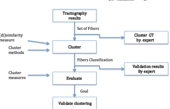
2.4 Tractography results . . . 27
3.1 Curvature . . . 46
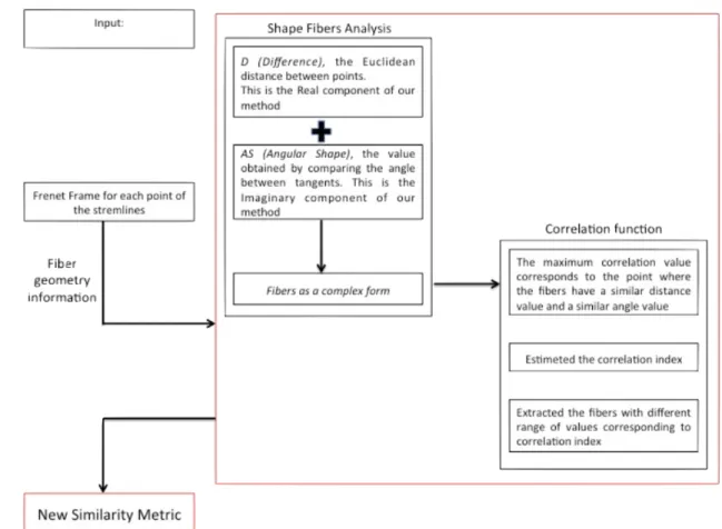
4.1 Framework of our method . . . 58
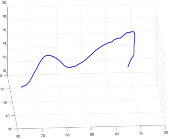
4.2 Streamline in 3D space . . . 61
4.3 Parameterization of the tract . . . 61
4.4 The cosine series representation at various degrees . . . 62
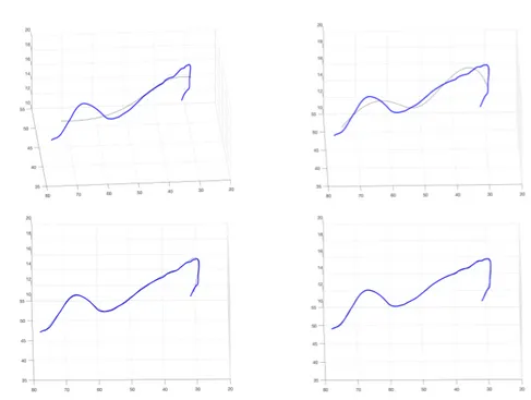
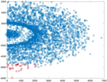
4.5 Range of Fibers with high correlation value (red area) . . . 66
4.6 Results of Fibers selected by the red area . . . 67
4.7 Range of Fibers with low correlation value (red area) . . . 67
4.8 Results of Fibers selected by the red area . . . 68
4.9 Range of Fibers with high correlation value (red area) . . . 68
4.10 Range of Fibers with low correlation value (red area) . . . 69
4.11 Results of Fibers selected by the red area . . . 69
4.12 Results of Fibers selected by the red area . . . 70
5.1 CA bundle . . . 74
5.2 CST bundle . . . 74
5.3 Fornix bundle . . . 75
5.4 Bundles of streamlines where fibers are spatial near (left) and far spatial (right) between them. . . 75
5.5 Fornix dataset. Clustering with Frechet metric. . . 77
List of Figures 1
5.7 Fornix and CA Dataset. The bundles are close to each other. Fornix dataset is composed of fibers whit different length and orientation. We considered it divided in two sides, right and left. The second dataset is CA, here the fibers have different lengths
but similar direction. . . 79 5.8 Fornix and CA dataset. Clustering with Frechet metric with
K-mean algorithm and k=2. . . 80 5.9 Fornix and CA dataset. Clustering with Frechet metric with
K-mean algorithm and k=3. . . 81 5.10 Fornix and CA dataset. Clustering with NewSimilarity metric with
K-mean algorithm and k=2. . . 82 5.11 Fornix and CA dataset. Clustering with NewSimilarity metric with
K-mean algorithm and k=2. . . 83 5.12 Fornix and CA dataset. Clustering with Frechet metric with
Agglomerative algorithm (numbers of cluster are two). . . 86 5.13 Fornix and CA dataset. Clustering with Frechet metric with
Agglomerative algorithm (numbers of cluster are three). . . 87 5.14 Fornix and CA dataset. Clustering with NewSimilarity metric with
Agglomerative algorithm (numbers of cluster are two). . . 88 5.15 Fornix and CA dataset. Clustering with NewSimilarity metric with
Agglomerative algorithm (numbers of cluster are three). . . 89 5.16 CST and CA Dataset. . . 91 5.17 CST and CA Fibers Clustering with Hausdorff metric, and
K-means algorithm (k=2). . . 92 5.18 CST and CA Fibers Clustering with Hausdorff metric, and
K-means algorithm (k=3). . . 93 5.19 CST and CA Fibers Clustering with NewSimilarity metric, and
K-means algorithm (k=2). . . 94 5.20 CST and CA Fibers Clustering with NewSimilarity metric, and
K-means algorithm (k=2). . . 95 6.1 Framework for a possible clinical application of distance metrics. . . . 100 6.2 At the top of the figure, the clinical case concerns the CST (left
and right); in the left figure is represented the CST (left and right) and the Arcuate left; otherwise in the right figure is represented
the CST and IFOF left. . . 102 6.3 Cluster result with K-means algorithm and Frechet metric. . . 104 6.4 Cluster result with K-means algorithm and NewSimilarity metric. . . 105 6.5 Cluster result with K-mean algorithm and Frechet metric. . . 107 6.6 Cluster result with K-mean algorithm and Hausdorff metric. . . 108 6.7 Cluster result with K-mean algorithm and LCSS metric.. . . 109 6.8 Cluster result with K-mean algorithm and NewSimilarity metric. . . . 110
1
Introduction
The human brain is the central organ of the human nervous system, and with the spinal cord makes up the central nervous system. It is the seat of recruitment, processing and transmission of information and the system of regulation of body functions. The brain directs the things we choose to do (like walking and talk-ing) and the things our body does without thinking (like breathtalk-ing). It is also in charge of sensing (sight, hearing, touch, taste, and smell), memory, emotions, and personality. Externally the brain is a soft, spongy mass of tissue. It is basically made up of two voluminous masses, the cerebral hemispheres, the surface full of pits and fissures that divide them into lobes. Internally a gray sub-stance and a white substance constitute it.
The gray matter is arranged peripherally and constitutes the cerebral cortex, while the white mat is in the center and consists of bundles of nerve fibers and of nuclei of gray matter, which are important nerve centers. The cerebral cortex is not functionally homogeneous, but divided into centers of localization, each one with different tasks. There is in fact a motor cortex, located in the frontal lobe, which processes and sends signals intended to produce the movements of the muscle groups; and a sensory cortex, which, placed in the parietal lobe, collects the stimuli from the periphery of our body.
With the use of brain imaging techniques, doctors and researchers have the opportunity to visualize behavior or clinical disorders within the human brain without recurring to invasive neurosurgery. There are a number of accepted, safe imaging techniques in use today in group facilities and hospitals throughout the world.
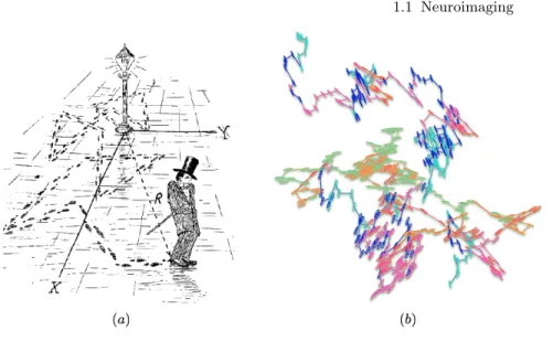
1.1 Neuroimaging
Neuroimaging or brain imaging is the use of various techniques to either directly or indirectly image the structure, function/pharmacology of the brain [24].
In 1918 the American neurosurgeon Walter Dandy introduced the technique of ventriculography [38]. X-ray [30] images of the ventricular system within the brain were obtained by injection of filtered air directly into one or both lateral ventricles of the brain. Dandy also observed that air introduced into the subarachnoid space
via lumbar spinal puncture could enter the cerebral ventricles and also demon-strate the cerebrospinal fluid compartments around the base of the brain and over its surface. This technique was called pneumoencephalography. Moniz [7], a neu-rologist, accomplished the first cerebral arteriogram in 1927, whereby both normal and abnormal blood vessels in and around the brain could be visualized with great precision. In the early 1970s, Allan McLeod Cormack and Godfrey Newbold Hounsfield introduced computerized axial tomography (CAT or CT scanning) [29], and ever more detailed anatomic images of the brain became available for diag-nostic and research purposes. Cormack and Hounsfield won the 1979 Nobel Prize for Physiology or Medicine for their work. Soon after the introduction of CAT in the early 1980s, the development of radioligands study of biomolecular behaviour, allowed single photon emission computed tomography (SPECT) [33] and positron emission tomography (PET) [9] of the brain. More or less concurrently, magnetic resonance imaging (MRI or MR scanning) [51] was developed by researchers in-cluding Peter Mansfield and Paul Lauterbur, who were awarded the Nobel Prize for Physiology or Medicine in 2003 [41]. In the early 1980s MRI was introduced clinically, and during the 1980s a veritable explosion of technical refinements and diagnostic MR applications took place. Scientists soon learned that the large blood flow changes measured by PET could also be imaged by the correct type of MRI. Functional magnetic resonance imaging (fMRI) [35] was born, and since the 1990s, fMRI has come to dominate the brain mapping field due to its low invasiveness, lack of radiation exposure, and relatively wide availability.
The ability to visualize anatomical connections between different parts of the brain, non-invasively and on an individual basis, has emerged as a major break-through for neuroscience’s Human Connectome Project [1] . More recently, a new field has emerged, diffusion functional MRI (dfMRI) [42] as it was suggested that with DWI (Diffusion Weighted imaging) [42] one could also get images of neuronal activation in the brain. Finally, the method of diffusion MRI has also been shown to be sensitive to perfusion, as the movement of water in blood vessels mimics a random process, intra-voxel incoherent motion (IVIM) [43]. IVIM dMRI is rapidly becoming a major method to obtain images of perfusion in the body, especially for cancer detection and monitoring. In diffusion weighted imaging, the intensity of each image element (voxel) reflects the best estimate of the rate of water diffusion at that location. Because the mobility of water is driven by thermal agitation and highly dependent on its cellular environment, the hypothesis behind DWI is that findings may indicate (early) pathologic change. For instance, DWI is more sensi-tive to early changes after a stroke than more traditional MRI measurements such as T1 or T2 relaxation rates. A variant of diffusion weighted imaging, diffusion spectrum imaging (DSI) [72], was used in deriving the Connectome data sets; DSI is a variant of diffusion-weighted imaging that is sensitive to intra-voxel hetero-geneities in diffusion directions caused by crossing fiber tracts and thus allows more accurate mapping of axonal trajectories than other diffusion imaging approaches. DWI is most applicable when the tissue of interest is dominated by isotropic water movement e.g. grey matter in the cerebral cortex and major brain nuclei, or in the body, where the diffusion rate appears to be the same when measured along any axis. However, DWI also remains sensitive to T1 and T2 relaxation. To entangle diffusion and relaxation effects on image contrast, one may obtain quantitative
im-1.1 Neuroimaging 3
ages of the diffusion coefficient, or more exactly the apparent diffusion coefficient (ADC) [44]. The ADC concept was introduced to take into account the fact that the diffusion process is complex in biological tissues and reflects several different mechanisms. Diffusion tensor imaging (DTI) [40] is important when a tissue such as the neural axons of white matter in the brain or muscle fibers in the heart has an internal fibrous structure analogous to the anisotropy of some crystals. Water will then diffuse more rapidly in the direction aligned with the internal structure, and more slowly as it moves perpendicular to the preferred direction. This also means that the measured rate of diffusion will differ depending on the direction from which an observer is looking. Traditionally, in diffusion-weighted imaging, three gradient-directions are applied, sufficient to estimate the different properties of diffusion tensor, for the measure of stroke. The principal direction of the dif-fusion tensor can be used to infer the white-matter connectivity of the brain (i.e. tractography; trying to see which part of the brain is connected to which other part). More extended DTI scans derive neural tract directional information from the data using 3D or multidimensional vector algorithms based on six or more gradient directions, sufficient to compute the diffusion tensor. The diffusion model is a rather simple model of the diffusion process, assuming homogeneity and lin-earity of the diffusion within each image voxel. Recently, more advanced models of the diffusion process have been proposed that aim to overcome the weaknesses of the diffusion tensor model. Amongst others, these include q-space imaging [39] and generalized diffusion tensor imaging.
1.1.1 Process of Diffusion
Diffusion is a passive form of material transport from areas of high concentration to areas of low concentration across a cell membrane. A distinguishing feature of diffusion is that it is dependent on particle random walk and results in mixing or mass transport, without requiring directed bulk motion.
The process of diffusion could be visualized by thinking of a drop of dark ink dropped into a glass of clear water. Initially, the ink appears to remain concentrated at the point of release. Gradually, some of the ink moves away from the region of high concentration, and instead of there being a dark region and a clear region, there is a graduation of color. After a long time, the ink is uniformly distributed in the water. The movement of the ink from the region of high concentration (ink drop) to the region of low concentration (the rest of the glass of water) is an illustration of the process of diffusion Figure(1.1).
Physis of Diffusion
There are two ways to describe the notion of diffusion: either a phenomenological approach starting with Fick’s laws and their mathematical solutions, or a physical and atomistic one, by considering the random walk of the diffusing particles [58]. From the atomistic point of view, diffusion is considered as a result of the random walk of the diffusing particles. In molecular diffusion, the moving molecules are self-propelled by thermal energy. Random walk of small particles in suspension in a fluid was discovered in 1827 by Robert Brown. In 1826 a botanist Robert
Fig. 1.1: Diffusion
Diffusion and Brownian Motion: on the left side of the figure, dark in into water can explain diffusion of ink in a fluid. On the right site of the picture trajectory of
molecules show the random pathways of free diffusion.
Brown was studying the seemingly random pattern of motion that pollen grains exhibited when suspended in water through his microscope [37]. Initially puzzled, he attributed it to some biological phenomenon of the pollen, but when he later observed the same behavior with inanimate, inorganic substances, he rejected this hypothesis. It later became clear that the motion that he had observed was due to the buffeting of the pollen grains by water molecules surrounding them. This led to the revelation that liquids and gases were not static and lifeless as they might appear at first glance. The atoms and molecules from which they are constituent are in constant motion, undergoing persistent collisions and energy exchanges with other molecules and atoms. This phenomenon was called Brownian motion. The theory of the Brownian motion and the atomistic backgrounds of diffusion were developed by Albert Einstein [3].
The physical and mathematical theories of diffusion were developed and refined over the next two centuries by prominent scientists including Thomas Graham [61] and Adolf Fick [69], who developed a rigorous mathematical framework, which is still in use today Figure(1.2).
In 1855 Adolf Fick described and solved the diffusion coefficient D [16] by means of the first diffusion law:
J = −Ddϕ
dx (1.1)
and the second diffusion law:
∂ϕ
∂t = D
∂2ϕ
∂x2 (1.2)
where J is the flux, ϕ is the concentration, D is the proportional coefficient between flux and concentration, t was time-variable, x was the displacement variable, in the one dimensional case. In 1.1, Fick relates the diffusive flux to the concentration under the assumption of steady state. It postulates that the flux goes from regions of high concentration to regions of low concentration, with the concept that a solute
1.1 Neuroimaging 5
Fig. 1.2: Random walk.
(a)Random walk according to Gamow; (b)Random walk trajectory due to Brownian motion in water.
will move from a region of high concentration to a region of low concentration across a concentration gradient. In 1.2, Fick predicts how diffusion causes the concentration to change with time.
In 1905 Albert Einstein, using Boltzmann’s thermal energy predictions [50], de-rived a rule to estimate Avogadro’s number by observing how far the polled grain moved over a given time. Einstein showed that the language of the Fick’s Law still applied in the cases of self-diffusion where no macroscopic gradient existed. He provided a formulation of local probability to find the molecule and he realized a correlation between thermal fluctuations and diffusion coefficient. Einstein’s ex-planation of Brownian motion was that the Brownian particles experience a net force resulting from the exterior collisions of surrounding water molecules. Einstein proved that the squared displacement of the particles from their starting point over a time, averaged over all of the sampled particles was directly proportional to the observation time; this formulation of diffusion model assumed that the medium was unrestricted and the particles therefore had equal mobility in every direction (free diffusion). The diffusion of particles inside fluids depends by the character-istics of the medium and obstacles characterize diffusion phenomena. Respect to the presence of preferable direction of molecules in their Brownian motion, we can define Figure(1.3):
• Anisotropic Diffusion, when a preferred direction is chosen by particles. This is typical in living tissues like fiber’s muscles and cell’s membranes. This means that obstacles characterize the medium as motion’s constrictor.
• Isotropic Diffusion, when no direction is preferred by diffusion process. Ink in free water shows that the medium is isotropic. This means that no barriers obstacle the Brownian motion of particles.
• Restricted Diffusion occurs when particles are linked by membranes and bar-riers obstacle the diffusion process.
• Hindered Diffusion occurs when particles are linked by surrounding object but barriers don’t obstacle diffusion propagation of molecules.
Fig. 1.3: Diffusion of particles
Picture a presents difference between anisotropic and isotropic diffusion (respectively left and right). Picture b show difference between restricted and hindered diffusion
respectively left and right).
1.1.2 Diffusion MR Tractography
Diffusion MR imaging [56] of the brain was first adopted for use in clinical neuro-radiology during the early 1990s and was found to have immediate utility for the evaluation of suspected acute ischemic stroke Figure(1.4).
Fig. 1.4: Diffusion MR tractography
Diffusion-weighted image (left) reflect water diffusion behavior (random walk) (right). Diffusion behavior is modulated by tissue structure at the cellular level (middle).
Since that time, enormous strides forward in the technology of diffusion imaging have greatly improved image quality and enabled many new clinical applications.
1.1 Neuroimaging 7
These include the diagnosis of intracranial pyogenic infections, masses, trauma, and so on. In neuroscience, tractography is a 3D modeling technique used to vi-sually represent neural tracts using data collected by difusion-weighted images. It uses special techniques of magnetic resonance imaging and computer-based im-age analysis. The results are presented in two-dimensional and three-dimensional images, Figure(1.5).
Fig. 1.5: MRI imaging
Results of MRI, in two-dimensional (left) and three-dimensional (right).
In addition to the long tracts that connect the brain to the rest of the body, there are complicated neural networks formed by short connections among dif-ferent cortical and subcortical regions. The existence of these bundles has been revealed by histochemistry and biological techniques on post-mortem specimens. Brain tracts are not identifiable by direct exam, CT, or MRI scans. This difficulty explains the paucity of their description in neuroanatomy atlases and the poor understanding of their functions.
Tractography can be considered a large class of algorithms that generate a bundle interpretation of Diffusion Processes in the brain. This means that trac-tography is an interpretation of anatomy with a different grade of accuracy based on diffusion data elaborations. Fibers are obtained by following the paths of par-ticles dropped in a vector field. The strategy used to approximate these paths constitutes the main difference between the methods analyzed.
White matter tractography algorithms can be classified into deterministic and probabilistic [8], [74]. The first only considers the main eigenvector direction in order to reconstruct the tract; the second class introduces the concept of pertur-bation in order to modify the vector direction at each location.
The deterministic approach produces a streamline that represents the main direction of diffusion for each voxel. This approach works well for many fiber bundles and can help to understand many configurations of lesion-pathways. The limit concerns the interpretation of voxels with low anisotropy. The Functional Anisotropy(FA) [10] interpretation is correct when voxels describe a region with-out any particular diffusion direction (ventricles). When a region is involved in fiber crossing, FA is around zero and the algorithm produces a wrong reconstruction (i.e. lateral portions of the corticospinal and corticobulbar tracts). The proba-bilistic approach aims to address this criticism by considering multiple pathways
moving from the seed point and from each point along the reconstructed trajecto-ries: the method accounts for the uncertainty in the estimation of fiber direction. Behind the probabilistic algorithm there are many pre-processing steps, such as co-registration, white matter extraction and statistical model estimation. This mean that it is very slow and non interactive.
Despite differences between strategies and algorithm implementation, the trac-tography procedure is based solving pathway equation [19]; common steps between different approaches are required to solve the pathway equation:
• Definition of seeds, the tracking process requires a starting point; this is typi-cally known as seed region, a collection of voxel defined in derived tensor map. Drawing seed region requires anatomical knowledge of fiber bundles and their localization. Alternative approaches can used label definition of the brain from external sources: using digital label atlas and parcellation method, it is possible to automatically set seeds. This method can be imprecise and computationally expensive.
• Selection of an integration strategy: different integration methods can be ap-plied in order to calculate pathways. The difference between them consists in the methodology of calculating the propagation direction and the step size. The most applied strategies are the Euler integration method, Runge-Kutta, Fiber Assignment by Continuous Tracking (FACT) and other alternative in-terpolation methods (Interpolated Streamline). As required for seed definition, stopping criteria determine when the tracking process has to finish. Thes meth-ods can be defined as a combination of limits imposed by used definition that interrupts calculation of fiber tracts. Some example of it are FA threshold, Angle Threshold, maximal length of fiber and number of iterations.
Deterministic algorithms use a linear propagation approach. Fiber trajectories are generated in a stepwise fashion deriving the direction of each step from the local diffusion tensor. Approaches of deterministic category are the following:
• Streamline approaches [20] generate fibers following the direction of faster diffusion (often main eigenvector). The propagation direction is described by a linear propagation of diffusion measurements. The main drawback appeared in areas where diffusion propagation was not linear, such as planar regions, since the trace of the fiber can not be determined in order to partial volume effects, such as crossing, kissing, and branching. FACT (Fiber Assignment by Continuous Tracking) algorithm altered the propagation direction at the voxel boundary interfaces. FACT algorithm used variable step sizes,depending upon the length of the trajectory needed to pass through a voxel. The tensor deflection approach (TEND) was proposed in order to improve propagation in regions with low anisotropy, such as crossing fiber regions, where the direction of fastest diffusivity is not well defined. The idea is to use the entire D to deflect the incoming vector direction and to obtain a smoother tract reconstruction result.
• The tensor line propagation method incorporates information about the voxel orientation, as well as the anisotropic classification of the local tensor given anisotropic indices. Tensor line propagation direction is a combination of the
1.2 Fibers Tractography 9
previous direction (main eigenvector) and the tensor deflection direction. Dif-fusion Toolkit and Trackvis are a famous couple of packages dedicated to diffusion tractography. The Diffusion Toolkit implements the most relevant deterministic algorithms such as the FACT, 2-order Runge Kutta, Interpo-lated Streamline and Tensorline. The Trackvis is the extraction software that calculates a sub-set of fiber bundle using ROI approaches.
Probabilistic fiber tractography algorithms aim to overcome bugs of determin-istic approaches by adding some random choice. Probabildetermin-istic fiber tracking can be considered a simulation protocol that describes random walk of particles through a set of voxels guided by tensor rules. For each seed points, probability algorithms trace different paths and calculate the spatial probability distribution of connec-tivity. Final tracking is the spectrum of possible paths.
1.2 Fibers Tractography
In clinical application, it is common practice to focus on selected white matter fiber bundles; these bundles represent major pathways in the overall physical connec-tivity of the brain, i.e., groups of fibers belonging to the same anatomical regions Figure(1.6).
Fig. 1.6: Anatomical Bundles
This image represent some of anatomical fibers bundle in the brain.
Identify the structures that compose the different part of the brain is an im-portant task in neuroimaging. One of the crucial points in neuroscience is image segmentation to partition the voxel into homogeneous subgroups that correspond to tissue types. Various techniques are proposed to segment fibers into meaningful anatomical structures for quantification and comparison between individuals.
Catani et al. [18] used a technique called virtual dissection to interactively select fibers passing through some manually defined regions of interests (ROIs). These approaches require a first manual intervention to select tracts of interest in a subset of subjects and then retrieve the same structure in other subjects, and making them unsuitable for a global WM segmentation. The manual identification of regions of interest is strongly affected by the prior knowledge used to identify the structures and very much prone to operator bias. Methods for the automatic
decomposition of whole brain tractography into fiber bundles could greatly help reduce complexity and bias associated with manual segmentation. This approach, frequently referred to as tractography segmentation, aims at generating a simpli-fied representation of the WM structure, enabling easier navigation and improved understanding of the structural organization of the brain and its overall connec-tivity. Though this technique is highly flexible, it is very time consuming due to a large amount of complex fiber structures. Moreover, the results may be biased by subjective opinions of experts.
Therefore, automatic fiber clustering algorithms, which require no user inter-action and thus exclude undesirable bias have gained considerable attention. Clus-tering approaches represent a logical alternative to supervised methods as they permit to discover bundle structures without the need of prior anatomical knowl-edge. Using tractography technique, white matter fiber tracts are represented as streamlines, which are sequences of points in 3D space. These streamlines can be grouped into fiber bundles, i.e., groupings of streamlines with similar spatial and shape characteristics, based on anatomical knowledge using clustering methods.
In the tractography literature we can find approaches which use unsupervised and/or supervised learning algorithms to create bundles. In supervised learning the data sets are divided into training and a test set. For the training set, experts will have provided anatomical labels for a set of manually segmented streamline bundles. The task is then to identify similar structures amongst the unlabeled streamlines in the test set. In unsupervised learning the focus is on creating a partitioning of the streamlines without knowing any labels. Several fiber-clustering approaches have been described in the literature of which their main goal is to analyze a collection of tractography fiber paths in 3D and separate them into bundles, by taking advantage of their similarity. Most automatic techniques for segmenting fibers are based on geometric properties of fibers. Two fibers are usually grouped into a bundle if a small distance separates them, have comparable length and have similar shape. However, these criteria might be insufficient, since two fibers with different shapes can be grouped into a bundle if they start and end at the same region. So, fiber segmentation remains an area of active research and a fiber similarity measure is also needed to cluster fibers. A fiber similarity measure is a function that computes the (dis) similarity between pairs of fibers.
1.3 Aims of thesis
Recognize the anatomic bundles within the brain is a very important task in the scientific community. It is important both in the diagnostic phase, because a good display of the subdivision of the areas of the brain may help the surgeon in the general view of the problem and in the intraoperative phase the importance of identifying the fascicles relies on the repute for a good result in neurosurgical re-section of the tumor, it is fundamental to preserve the areas of the main functional activities. Despite advances in the field of neuroimaging, this task is not easy to implement. There are many aspects to consider in order to get a good clustering algorithm that allows splitting the fibers of the brain in anatomical bundles.
Currently the surgeons, during surgery, make use of neuronavigation as a support tool. Neuronavigation represents the new frontier of minimally invasive
1.3 Aims of thesis 11
surgery. A neuronavigation tool allows the surgeon to perform brain surgery with extreme accuracy and speed. Intraoperatively, the system shows on MRI or CT the tool position thus solving the first problem of the surgery, which is the spatial ori-entation of the anatomy. The possibility of preliminary planning the intervention and the help of a computer during the procedure create a new approach on how to consider the brain leading to innovative methods of surgical procedures. Through the use of neuron-navigation it is possible to identify the best path and the area where to attack the pathology considering its three-dimensional appearance and movements of adjacent structures.
As described above:
• From MR data, the white matter fiber tract can be reconstructed using a class of technique called tractography.
• The dataset derived by tractography is composed of a large number of stream-lines, which are sequences of points in 3D space. To simplify the visualization and analysis of white matter fiber tracts obtained from MR data, it is often necessary to group them into larger clusters or bundles.
• In order to perform clustering, first a mathematical definition of fiber similarity (or more commonly a fiber distance) must be specified. Then, pairwise fiber distance may be calculated and used as input for a clustering algorithm. The main problems that we are analyze:
• Define a relevant metric to assess the similarity of tracts. • Establish the right number of clusters.
• Evaluate, once the clusters are obtained, qualitatively the results.
The final goal of this analysis is to obtain a new metrics for brain fiber classifi-cation. In literature various distance similarity measures are used; some methods calculates the similarity of the fiber point to point but these procedures are sen-sitive to noise, which affects the final distance similarity between pairs of fibers. The final distance alone between two fibers is not enough to tell whether they have a similar shape or they are separated by a small distance. Thus, this limits their ability to effectively group fibers into meaningful bundles. Another point is that the most common techniques have quadratic time complexity, is a problem for large fiber data sets. Several techniques are proposed to measure the shape similarity of two fibers; they also are efficient and robust to noise within fibers, but the complexity is still quadratic time.
Distance study during the last years captures the local relationship between pairwise fiber tracts but tend to lack the ability to captures the global structure of fiber tracts such as the shape variability and the neighborhood structures. In order to provide such information, the purpose of our proposed method, named "NewSimilarity" metric, is to developed a metric where both distance and shape information are considered during the clustering. The results obtained with our similarity metric confirm a good shape classification of the fibers of the brain.
In subsequent sections, we analyze the similarity metrics between fibers best known in the literature and we study the main clustering methods.
After this introduction, this thesis is organized as follows: • Chapter 2 : State Of the Art
Overview of the distance metrics between the fibers and the clustering algo-rithms used in the literature.
To simplify the visualization and analysis of white matter fiber tracts obtained from diffusion Magnetic Resonance Imaging data, it is often necessary to group fibers into larger clusters, or bundles. One approach is based on the knowledge of experts and is referred to as virtual dissection; it often requires several inclusion and exclusion regions of interest that make it a very hard process to reproduce across expert. Manual segmentation is very time consuming, is strongly user-dependent and adds biases to tract-based analyses.
For this reason, it is preferable to use fiber clustering algorithms, which use distance metrics to classify the fibers in the different anatomical bundles. • Chapter 3 : Mathematical Background
Overview of the mathematical foundations necessary in order to understand our method of studying the shape and classification of fibers.
In particular we describe the properties to be verified by our metrics and how similarity metrics (or dissimilarity) are applied to clustering algorithms. • Chapter 4 : Method for our processing of create NewSimilarity metric
New frameworks of clustering techniques and distance measures.
The most common measures used for distance only capture the local rela-tionship between streamlines but not the global structure of the fiber. Global structure, refer to the fiber variability shape. Together, local and global in-formation, may define a good measure of similarity. In order to provide such information, we developed a novel framework where both distance and shape information are considered during the clustering.
• Chapter 5 : Experimentals
As a first step we consider datasets available online by ISMRM 2015 Trac-tography challenge-Data. TracTrac-tography challenge was based on an artificial phantom generated using the Fiberfox software, based on bundles segmented from a HCP subject.
• Chapter 6 : Algorithm verification with clinical data
In the following we show the results obtained by analyzing, as a first step, only the step related to the similarity metric. The clinical data used have been previously processed using the tractography algorithms and the bundles have already been segmented. The purpose is to understand which is the distance metrics that offers, compared to a ground truth, the best recognition of the different anatomical bundles. We also want to see if the metrics applied to online data are also applicable to clinical data. Afterwards we will summarize in a table the results obtained by applying the selected metrics to the clinical datasets and how clustering occurs in the different cases. We will present in detail the most significant cases. We use the library in Python, ?scikit-learn? for clustering classification.
2
State of the Art
After pre-processing images and fit a diffusion model at every voxel, the fiber tracts can be virtually reconstructed or traced throughout the brain using computational methods called tractography. It is a method to reconstruct the pathways of ma-jor white matter fiber bundles, by fitting a curved path through the directional diffusion data at each voxel.
Deterministic tractography recovers fibers emanating from a seed voxel by fol-lowing the principal direction of the diffusion tensor or the dominant direction of the diffusion orientation distribution function (ODF). However, this method has limitations: it depends on the choice of initial seed points and can be sensitive to the estimated principal directions. To overcome those drawbacks, probabilistic tractography methods have been proposed.
They can be computationally more intensive but can be more robust to partial volume averaging effects and uncertainties in the underlying fiber direction, which are inevitable due to imaging noise. Regardless of the chosen type, the analysis produces a large number of fibers that need to be grouped into anatomical bundles. To simplify the visualization and analysis of white matter fiber tracts obtained from diffusion Magnetic Resonance Imaging data, it is often necessary to group them into larger clusters, or bundles. One way is based on the knowledge of experts and is referred to as virtual dissection; it often requires several inclusion and exclu-sion regions of interest that make it a process that is very hard to reproduce across expert. Manual segmentation is very time consuming, is strongly user-dependent and adds biases to tract-based analyses. For this reason, it is preferable to use fiber clustering algorithms, which use distance metrics to classify the fibers in the different anatomical bundles.
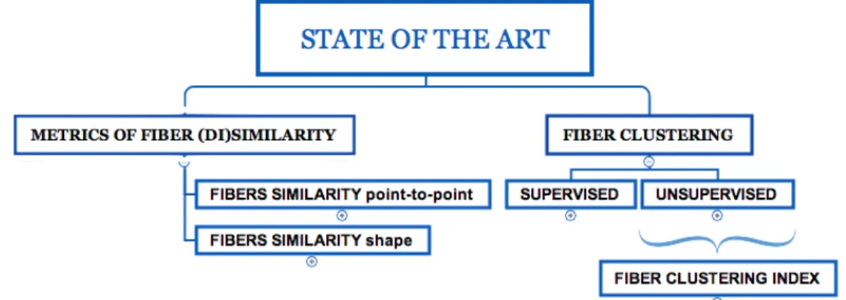
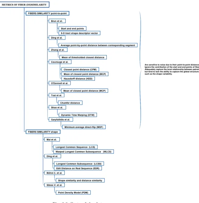
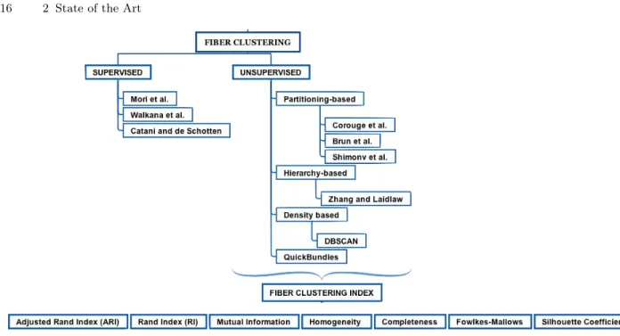
An overview of the distance metrics between the fibers and the clustering al-gorithms used in the literature is shown in Figure(2.1) where we have a general overview of the ingredients necessary for the study of a new similarity metric; in Figure(2.2) and Figure(2.3) we will see in detail, the similarity metrics and the clustering algorithms, used in the literature.
Fig. 2.1: State of the Art
Metrics of fiber (di)similarity and Fiber Clustering. Overview of the ingredients necessary for the study of a NewSimilarity metric.
2.1 Metrics of fiber (di)similarity: fibers similarity
point-to-point and fibers similarity shape
A typical framework for fiber clustering defines a pairwise similarity/distance be-tween each pair of fibers in a large set of candidate fibers, to group them into separate and distinct tracts. In order to perform clustering, first a fiber similarity measure must be specified, which is then used as input to a clustering algorithm. A fiber similarity measure is a function that computes the (dis)similarity between pairs of fibers. Two fibers are considered similar when they have comparable length, similar shape and are separated by a small distance.
Distances between pairwise fibers Fiand Fjare used for the similarity measure:
• Brun et al [5] considere the measure of similarity based on the idea that two fibers with similar end points should be considered similar. Euclidean distance between the end points of fibers is then used to calculate the fiber similarity. This similarity measure works fine in most cases where the fibers are not broken and really connect different parts of the brain in an anatomically correct way. This point is a great limitation because the white matter tracts contain many spurious and noisy fibers which do not allow an efficient calculus measure of similarity.
The assumption done by Brun is not reasonable in many cases since not all fiber bundles start and end in the same regions.
2.1 Metrics of fiber (di)similarity: fibers similarity point-to-point and fibers similarity shape 15
Fig. 2.2: State of the Art
Fig. 2.3: State of the Art
Fiber Clustering and Index. Review of principal clustering algorithms used in literature.
• Later Brun et al. introduced a 9-D tract shape descriptor vector, defined as the mean and lower triangular part of the covariance matrix of the points on a fiber, and computed the Euclidean distance between shape descriptors [4]. It ignores the information of most other points and the fiber pairwise shape similarity.
• Corouge et al [32] form point pairs by mapping each point of one fiber to the closest point on the other fiber; the distance between the pairs of fibers is calculated using these points. Three distances are defined; the first one is the closest point distance:
dc(Fi, F j) = minpk∈Fi,pl∈Fj||pk− pl||
with || · || being the Euclidean norm (2.1)
It is the minimum distance between a pair of points. These distance cannot be expected to have a good discrimination power between fibers since it encodes only very raw information about fiber similarity and closeness.
The second distance is the mean of closest point distances (MCP): dM(Fi, F j) = mean(dm(Fi, Fj), dm(Fi, Fj))
with dm(Fi, Fj) = meanpl∈Fiminpk∈Fj||pk− pl||
(2.2) which calculates the average of the points pair distances. The minimum dis-tance provides a global similarity measure integrated along the whole curve.
2.1 Metrics of fiber (di)similarity: fibers similarity point-to-point and fibers similarity shape 17
The last measure is the Hausdorff distance (HDD): dH(Fi, Fj) = max(dh(Fi, Fj), dh(Fi, Fj)))
with dh(Fi, Fj) = maxpk∈Fiminpl∈Fj||pk− pl||
(2.3) that is the maximum distance between a pair of points.
Being a worst-case distance, the Hausdorff distance is a useful metric to reject outliers and prevents the algorithm from clustering curves with high dissimi-larity.
• Zhang and Laidlaw [76] define the mean of thresholded closest distances; the distance between two fibers as the average distance from any point on the shorter fiber to the closest point on the longer fiber, and only distances above a certain threshold contribute to this average.
• The average point-by-point distance between corresponding segment is defined by Ding et al. [22]. Their fiber similarity measure is then defined as the mean distance between the corresponding segments.
When two fibers are similar in shape and close in location these distance is small; when the distance between a pair of fibers is large, or their shapes are different, the distance is large. To define piece-wise similarity, the authors use the mean Euclidean distance between the segments. This similarity method is efficient but not effective since this measure also loses the point-by-point information.
• The distance measure such as closest point distance, Chamfer distance [26]: D(Fi, Fj) = 1 |Fi| X Fip∈Fi minFjq∈Fj||Fip− Fjq|| with Fi= Fip p = 1, Fj= Fjq q = 1
where p,q are the set of points on a fiber Fi, Fj
|| · || Euclidean norm
(2.4)
and Hausdorff distance [31], have been the most used that adequately capture the local relationship between pairwise fiber tracts.
In [46] the authors propose a novel approach for measuring the similarity of 3D curves in a large dataset that includes the whole information of the curve for more accurate clustering and further quantitative analysis.
In [6] a manifold learning approach to fiber tract clustering is using. To gen-erate the similarity measure, the Chamfer and Hausdorff distance are initially employed as a local distance metric to construct minimum spanning trees be-tween pairwise fiber tracts.
All these distances lack the ability to capture the global structure of fiber tracts such as the shape variability and the neighborhood structures. In [53] several distance measures are implemented for fiber evaluation and the authors concluded that the mean of closest distances performs better than closest point distance, Hausdorff distance and end point distance.
• Shao et al. [34] extended the idea of the functions proposed by Courouge, using Dynamic Time Warping (DTW):
ddtw(Fi, Fj) = ||pn− qm|| + min(ddtw(fin−1, fjm), ddtw(fin, fjm−1), ddtw(fin−1, fjm−1))
with Fi= (p1, ..., pn), Fj= (q1, ..., qm)
(2.5) due to its flexibility with varying length fibers. It is a technique that looks for the optimal alignment of two time series.
• Garyfallidis et al. [23] used Minimum average Direct-Flip (MDF) distance: M DF (F, t) = min(ddirect(F, t), df lipped(F, t))
ddirect(F, t) = d(F, t) = 1 K X K i = 1|Fi− ti|
df lipped(F, t) = d(F, tf lip) = d(Ff lip, t)
(2.6)
which is a symmetric distance function that can address with the streamline bi-directionality problem. The direct distance ddirect(F, t)between two
stream-lines F ,t is the mean of the Euclidean distances between corresponding points. MDF can be applied only when both streamlines have the same number of points.
The main advantages of the MDF distance are that it is fast to compute, it takes account of streamline direction issues through consideration of both direct and flipped streamlines.
The distance measures similar to those mentioned above:
• Are sensitive to noise due to their point-to-point distance mechanism which affects the final distance similarity between pairs of fibers.
• Ignore the contribution of the start and end points of fibers which play an important role in the segmentation.
• Adequately capture the local relationship between pairwise fiber tracts but tend to lack the ability to capture the global structure of fiber tracts such as the shape variability and the neighborhood structures, due to the complexity of fiber structure.
• Their quadratic time complexity makes them hard to deal with large fiber datasets.
For these reason other approaches are being studied. These metrics, compared to previous metrics, are better to an analysis of fibers regarding the shape.
Two key aspects for achieving effectiveness and efficiency when managing time series data are representation methods and similarity measures. Time series are essentially high dimensional data and directly dealing with such data in its raw format is very expensive in terms of processing and memory cost. The best known of such distance is the Longest Common Subsequence (LCSS) distance [47]:
LCSS(M BEδ,ε(A), B) =
n
X
i=1
(2.7) that utilizes the longest common subsequence model. Given a time constrain δ and a similarity threshold ε, the lower bounding distance of LCSSδ,ε(A, B)of two
2.1 Metrics of fiber (di)similarity: fibers similarity point-to-point and fibers similarity shape 19
A(M BEδ,ε(A))with respect to the time constraint δ and the similarity threshold
ε.
To adapt the concept of matching characters in the settings of time series, a threshold parameter was introduced, starting that two different points from two time series are considered to match if their distance is less than the parameter.
Edit Distance on Real sequence (EDR) [27], given two trajectories R and S of lengths n and m, respectively the distance between R and S is the number of insert, delete, or replace operations that are needed to change R into S,
EDRε(R, S) =
edrε(R, S)
max(n, m) (2.8)
Similar to LCSS, EDR also uses a threshold parameter, except its role is to quantify the distance between a pair of points to 0 or 1.
• Mai et al. [67] introduce a novel similarity model called SIM for fiber segmen-tation, using a so-called fiber envelope. Based on this scheme, some new shape similarity techniques are proposed by adapting existing similarity techniques for trajectory data such as those mentioned before, Warped Longest Common Subsequence (WLCS) is one of these.
Given a time constrain δ and a similarity threshold ε, the similarity between two sequences A, B, with time points n, m is:
W LCδ,ε(A, B) = 1 −
wlcsδ,ε(A,B)
n, m (2.9)
is more accurate and more robust to noise and local time shifting within fibers than other similarity measures.
• Böhm C. et al [15], propose a novel similarity measure for fiber clustering by combining shape similarity and distance similarity into a unified and flexible method.
LCSS is specially adapted to points in three-dimensional space to measure shape similarity, and is less sensitive to noise than other distance based meth-ods. In addition, the distance between start and end points of a pair of fibers, which is referred to as distance similarity, is also incorporated to effectively capture the complex notion of fiber similarity.
As a result, our approach provides an effective and flexible way to the similarity between fibers.
• Siless V. et al [64], propose tu use the Point Density Model (PDM) metric. Given a fiber X, it is represented as the sum of Dirac concentrated at each fiber point, respect to fiber Y :
P DM2(X, Y ) = ||X||2+ ||Y ||2− 2hX, Y i (2.10)
Whereas PDM time complexity is quadratic in the number of points per fiber, using it for computing a full distance matrix is too expensive time-wise. By using multidimensional scaling the authors only compute a partial distance matrix and embed this information in a new set of fiber-like points. PDM is sensitive to the fibers form and position and is quite robust to missing fiber segments.
This last property is much desired as fibers are often mis-segmented due to noise and crossing fibers issues. MDF distance and PDM distance require us to resample tracts so that they have the same amount of points each. Hausdorff and Mean Closest Point work for tracts with different amounts of points.
2.2 Fiber Classification
Diffusion-Weighted Magnetic Resonance Imaging is one of the most used tech-niques for the analysis of the human brain white matter. Tractography datasets, composed of a big set of 3D streamlines, can be reconstructed from dMRI and represent the main anatomical connections in the brain.
There are two ways for analysis of dMRI tractography data generatting a quan-titative description of the white matter connections. The first method, fiber clus-tering, describes the connections of the white matter as clusters of fiber trajecto-ries. The clusters give anatomical regions in which properties of the white matter structure may be measured.
The second method is parcellation-based and uses tractography to estimate the "structural connectivity" between pairs of parcellated cortical regions. The pairwise connectivities are encoded in a matrix that models networks in the brain. These two types of analysis of dMRI tractography data both perform a seg-mentation of the white matter, but with different goals.
Parcellation-based approaches for white matter segmentation address the ques-tion of what regions a fiber trajectory may connect. These approaches take advan-tage of additional information in the form of a cortical parcellation into regions of interest (ROIs) that define network nodes, enabling analysis of the brain as a net-work. Once the nodes are defined, segmentation of tractography is straightforward and is based simply on connections between ROIs.
Clustering approaches generally address the goal of detecting the central, anatomically named portions of each fiber tract, without reference to cortical re-gions. These approaches do not enable graphical analysis of the brain networks, but rather focus on measuring properties of the anatomy of the fiber tracts. Early work in tractography clustering had the goal of organizing the fibers within a single subject into fiber tracts or bundles.
In the literature this problem is divided into two parts:
• choice of similarity or distance metric for comparing fibers (methods explained in the previous section)
• choice of clustering method
In the following section, we especially focus on reviewing the fiber clustering meth-ods, which is the scope of our work.
2.2.1 Fiber Clustering: Supervised and Unsupervised
In a supervised setting, the classes are a predetermined finite set. A learning data set is labeled with the classifications. The task of the algorithm is to find predictive patterns and build mathematical models to relate those to the known classification.
2.2 Fiber Classification 21
Unsupervised algorithms do not start with a classification; they search for similarities in the data to determine if they can be characterized as belonging to the same group. In an unsupervised setting, or "cluster analysis", the algorithm does not rely on any information on how elements are grouped and its task is to group them. Several methods have been proposed to obtain the clear fiber bundles representation.
We analyze as first step the Supervised methods: the identification of fiber bundles is carried out via manual identification of regions of interest corresponding to the main known pathways. The three mains algorithms of this type are:
• Mori et al. [54] • Wakana et al. [71] • Catani et al. [17]
However, these technique requires a priori knowledge about the trajectory and can be used only for well-characterized white matter tracts.
To reduce the complexity of manual segmentation and reduce the errors in-troduced by it, methods are inin-troduced for the automatic decomposition of whole brain tractography into fiber bundles. For this reason over the years, many semi-automatic methods have been studied in the scientific community for determining the bundles within and across subjects with little or no human intervention.
This approach, frequently referred to as tractography segmentation, aims at generating a simplified representation of the white matter structure, enabling easier navigation and improved understanding of the structural organization of the brain and its overall connectivity.
To automate bundles retrieval, various methods, based on different strategy were proposed over the last few years. The solution proposed in Li et al. [45] is an evolution of the ROI-based technique that works directly on fiber and applies prior knowledge to perform preliminary parcellation of the brain. A nonlinear method of kernel-principal component analysis (PCA) is used to project the fiber curves onto the principal component space of the kernel vectors.
Then, a fuzzy c-mean algorithm is applied to automatically group the fibers in the feature space. However, this approach is limited by the level of detail of the brain atlases, which can prevent the retrieval of small structures or suffer from cross-subject misalignments.
Other methods were also proposed to recover local white matter bundles using prior knowledge. Mayer et al. [49] presented a supervised framework for the auto-matic registration and segmentation of white matter tractography extracted from brain diffusion magnetic resonance imaging.
The framework relies on the direct registration between the fibers, without requiring any intensity-based registration as preprocessing. An affine transform is recovered together with a set of segmented fibers. These approaches require a first manual intervention to select tracts of interest in a subset of subjects and then retrieve the same structure in other subjects, and making them unsuitable for a global white matter segmentation.
The second method for fiber classification is "Unsupervised". Indeed clustering approaches represent a logical alternative to supervised methods as they permit to discover bundle structures without the need of prior anatomical knowledge.
In unsupervised method, we can classify the clustering techniques on the basis of the type of algorithm used to divide space:
• 1 Partitioning methods.
A partitioning method first creates an initial set of k partitions, where, pa-rameter k is the number of partitions to construct. It then uses an iterative relocation technique that attempts to improve the partitioning by moving ob-jects from one group to another. These clustering techniques create a one-level partitioning of the data points.
The best known algorithms in this area are K-means, K-medoids and fuzzy C-means. The clusters are formed according to the distance between data points and cluster centers are formed for each cluster. The number of clusters ( k-value) is specified by the user. The data points in each cluster are displayed by different colors, one color for one cluster.
K-Means is one of the simplest unsupervised learning algorithms that solves the well known clustering problem. The procedure follows a simple and easy way to classify a given data set through a certain number of cluster fixed a priori.
The main idea is to define k centroids, one for each cluster. These centroids should be placed in a cunning way because of different location causes different result. So, the better choice is to place them as much as possible far away from each other.
The next step is to take each point belonging to a given data set and associate it to the nearest centroid. When, no point is pending, the first step is completed and an early group age is done. At this point it is necessary to re-calculate k new centroids as bar centers of the clusters resulting from the previous step. After obtaining these k new centroids, a new binding has to be done between the same data set points and the nearest new centroid.
A loop has been generated. As a result of this loop, one may notice that the k centroids change their location step by step until no more changes are done. K-means is a simple algorithm that has been adapted to many problem domains and it is a good candidate to work for a randomly generated data points. One of the most popular heuristics for solving the K-means problem is based on a simple iterative scheme for finding a locally minimal solution.
The basic strategy of K-medoids clustering algorithms is to find k clusters in nobjects by first arbitrarily finding a representative object (the medoids) for each cluster.
Each remaining object is clustered with the medoid to which it is the most sim-ilar. K-medoids method uses representative objects as reference points instead of taking the mean value of the objects in each cluster.
The algorithm takes the input parameter k, the number of clusters to be partitioned among a set of n objects.
Traditional clustering approaches generate partitions; in a partition, each pat-tern belongs to one and only one cluster.
Hence, the clusters in a hard clustering are disjoint. Fuzzy clustering extends this notion to associate each pattern with every cluster using a membership function.
2.2 Fiber Classification 23
The output of such algorithms is a clustering, but not a partition. Fuzzy clus-tering is a widely applied method for obtaining fuzzy models from data. It has been applied successfully in various fields including geographical surveying, finance or marketing.
K-means algorithm is efficient for smaller data sets and K-medoids algorithm seems to perform better for large data sets.
The performance of Fuzzy clustering is intermediary between them. It produces close results to K-means clustering, yet it requires more computation time than K-means because of the fuzzy measures calculations involved in the algorithm. • 2 Hierarchical methods.
A partitional clustering is a simply a division of the set of data objects into non-overlapping subsets such that each data object is in exactly one subset. A hierarchical clustering is a set of nested clusters that are organized as a tree. Hierarchical clustering algorithm is of two types, Agglomerative Hierarchical clustering algorithm and Divisive Hierarchical clustering algorithm; both this algorithm are exactly reverse of each other.
Agglomerative Hierarchical clustering works by grouping the data one by one on the basis of the nearest distance measure of all the pairwise distance between the data point. Again distance between the data point is recalculated but which distance to consider when the groups has been formed. There are many available methods, some of them are single linkage, complete linkage, average linkage and centroid distance.
The advantages of this method is no a-priori information about the number of clusters required and are easy to implement and gives best result in some cases.
As disadvantages, the algorithm can never undo what was done previously, time complexity, sensitivity to noise and outliers and breaking large clusters. • 3 Density-Based.
In density-based clustering, clusters are defined as areas of higher density than the remainder of the data set. Objects in these sparse areas are usually con-sidered to be noise and border points.
The most popular density based clustering method is DBSCAN. In contrast to many newer methods, it features a well-defined cluster model called "density-reachability". Similar to linkage based clustering, it is based on connecting points within certain distance thresholds. However, it only connects points that satisfy a density criterion, in the original variant defined as a minimum number of other objects within this radius.
A cluster consists of all density-connected objects (which can form a cluster of an arbitrary shape, in contrast to many other methods) plus all objects that are within these objects’ range.
Another interesting property of DBSCAN is that its complexity is fairly low - it requires a linear number of range queries on the database - and that it will discover essentially the same results (it is deterministic for core and noise points, but not for border points) in each run, therefore there is no need to run it multiple times.
Mean-shift is a clustering approach where each object is moved to the densest area in its vicinity, based on kernel density estimation. Eventually, objects
con-verge to local maxima of density. Similar to k-means clustering, these "density attractors" can serve as representatives for the data set, but mean-shift can detect arbitrary-shaped clusters similar to DBSCAN.
Due to the expensive iterative procedure and density estimation, mean-shift is usually slower than DBSCAN or k-Means. Besides that, the applicability of the mean-shift algorithm to multidimensional data is hindered by the unsmooth behaviour of the kernel density estimate, which results in over-fragmentation of cluster tails.
A common clustering framework is based on the exploitation of the affinity matrix of a single subject that indicates the similarity between each pair of fibers: • Brun et al. [4] present a framework for unsupervised segmentation of white
matter fiber traces obtained from diffusion weighted MRI data.
Fibers are compared pairwise to create a weighted undirected graph which is partitioned into coherent sets using the normalized cut criterion. The points to be clustered are represented by a undirected graph, where the nodes correspond to the points to be clustered and each edge represent the similarity between points. The cut is a graph theoretical concept which for a partition of the nodes into two disjunct sets.
• O’Donnell et al. [55] use the eigenvectors of the similarity matrix. An eigen-vector is a eigen-vector that when multiplied by the matrix, still points in the same direction.
The authors used the top eigenvectors of the fiber similarity matrix to calculate the most important shape similarity information for each fiber path while removing noise. For each fiber path, this information could be visualized as a point, to show the separation of clusters according to similarity.
• Zhang et al. [75] used the agglomerative hierarchical clustering method and defined the distance between two clusters as the minimum proximity value between any two curves from two clusters.
A limitation common to all algorithms based on affinity matrix is their propensity to suffer from computational load owing to the calculation of pairwise distances between streamlines.
Approaches to reduce computational complexity have been proposed like: • Quick Bundles (QB) [23]. This method overcomes the complexity of these large
data sets and provides informative clusters in seconds.
Each cluster can be represented by a single centroid streamline, collectively these centroid streamlines can be taken as an effective representation of the tractography. QB is a surprisingly simple and fast algorithm which can reduce tractography representation to an accessible structure in a time that is linear in the number of streamlines.
The streamlines, are a fixed-length ordered sequence of points.
• Demir et al. [21] adopt the scenario of clustering data streams into the fiber clustering framework.
Existing clustering methods often suffer from the burden of computing pairwise fiber (dis)similarities, which escalates quadratically as the number of fiber pathways increases. To address this challenge, the authors propose to use an
2.3 Validation 25
online hierarchical clustering method, which yields a framework similar to doing clustering while simultaneously performing tractography.
• Ros et al. [60] uses a hierarchical cluster analysis approach that exploits the inherent redundancy in large datasets to time-efficiently group fiber tracts. Structural information of a white matter atlas can be incorporated into the clustering to achieve an anatomically correct and reproducible grouping of fiber tracts.
This approach facilitates not only the identification of the bundles correspond-ing to the classes of the atlas; it also enables the extraction of bundles that are not present in the atlas.
• In Guevara et al. [25], the authors describe a sequence of algorithms performing a robust hierarchical clustering that can deal with millions of diffusion-based tracts. The end result is a set of a few thousand homogeneous bundles. This simplified representation of white matter that can be used further for group analysis.
The bundles can also be labelled using ROI-based strategies in order to perform bundle oriented morphometry.
The methods described above, have been proposals to automatically estimate the number of cluster from the dataset. However, the results of this approach are strongly conditioned by the number of hierarchical steps and several input param-eters are required to carry out a comprehensive map of white matter bundles.
2.3 Validation
Clinical applications of diffusion MR fibre tractography tend to be more concerned with the anatomical trajectory of the fibres rather than structural or functional connectivity, i.e. to determine the exact spatial location of white matter pathways in the human brain.
For clinical application it is therefore not only important to validate what white matter pathways connect to what brain region, but also validate their exact course through the brain. In following, we will discuss of methods available for validation of the precise anatomical trajectory of diffusion MR fibre tractography and we address their benefits and drawbacks.
One more challenges still remaining in validating tractography is defining a proper evaluation metric for comparing the tractography results with the estab-lished ground truth. Fibre tractography in its current state is inherently limited by the spatial resolution of MRI and noise.
Tractography results are therefore unlikely to exactly coincide with the true anatomy. If we want to compare the performance of fibre tractography algorithms, we not only need to establish a ground truth, but also require a metric to compare the performance. A common metric in image analysis with respect to segmentation is the use of volume overlap to determine how well two segmentations coincide.
One common approach to validating the accuracy and performance of clinical scanners of any kind is the use of physical phantoms.