The cost-quantity relations and the diverse patterns of 'learning by doing': Evidence from India

Contents lists available atScienceDirect

Research Policy

journal homepage:www.elsevier.com/locate/respol

The cost-quantity relations and the diverse patterns of

“learning by doing”:

Evidence from India

Giovanni Dosi

, Marco Grazzi

, Nanditha Mathew

a_{Institute of Economics, Sant’Anna School of Advanced Studies, Piazza Martiri della Liberta 33, 56127 Pisa, Italy} b_{Department of Economics, University of Bologna, Piazza Scaravilli 2, 40126 Bologna, Italy}

c_{IBIMET-National Research Council, Via Giovanni Caproni, 8, 50145 Florence, Italy}

A R T I C L E I N F O

A B S T R A C T

“Learning-by-doing” is usually identified as a process whereby performance increases with experience in pro-duction. Of course such form of learning is complementary to other patterns of capability accumulation. Still, it is fundamental to assess its importance in the process of development. The paper investigates different patterns of“learning by doing”, studying learning curves at product level in a catching-up country, India. Cost-quantity relationships differ a lot across products belonging to sectors with different “technological intensities”. We find also, puzzlingly, in quite a few cases, that the relation price/cumulative quantities is increasing. We conjecture that this is in fact due to quality improvement and‘vertical’ product differentiation. Circumstantial evidence rests on the ways differential learning patterns are affected by firm spending on research and capital invest-ments. Finally, our evidence suggests that“learning”, or performance improvement over time is not just a by-product of the mere repetition of the same by-production activities, as sometimes reported in previous studies, but rather it seems to be shaped by deliberatefirm learning efforts.

1. Introduction

Theoretical and empirical studies in economics consider “learning-by-doing” as a process in which an increase in experience in a particular type of production (‘doing’) yields an improvement in efficiency (‘learning’). Typically the postulated relation is a power law, linking some performance indicator (e.g. unit costs, unit prices, productivity) with an experience indicator (e.g. cumulated production). The evi-dence, which we shall review below is quite robust. However the simplified version of “learning by doing”, henceforth LBD, presents significant drawbacks. First, LBD, as shown in the innovation literature is only one of several, often complementary forms of knowledge accu-mulation. Second, even when strictly applies, as discussed by, for ex-ample, Scott-Kemmis and Bell (2010), it is often considered that learning is a costless activity and an automatic by-product of continued production activities. Third, it is generally assumed that all organiza-tions have the same capacity to learn and there are no differences in absorptive capacities that might lead to differences in the intensity of learning across different organizations. Fourth, only rarely the product characteristics remain in actual fact invariant. Rather, often, the object of ‘learning’ improves its performance but at the same time, its pro-duction costs.

In this work we investigate the existence, shape and slope of learning curves in a developing country, namely India, at the product-level, conditioning onfirms’ and sectoral characteristics. In particular, we shall analyze,first, how the slope of the learning curves are affected by R & D andfixed investment activities, and second, by the timing of entry of thefirm in any one production activity, and hence, indirectly by the positioning of thefirm along the life cycle of a product (and thus, the possible knowledge spillovers it gains from older incumbents). Needless to say, the understanding of the determinants of the very ex-istence and slope of learning curves is not only important in its own right as a part of the microeconomics of innovation, but bear far reaching implications for the very analysis of the determinants of growth– in general and especially with respect to emerging economies. For example, would one find widespread and relatively uniform learning curves, that would give support to the view whereby knowl-edge is simply the “unintentional side effect of the production of a conventional good” (Romer, 1990) and, dynamically, the notion that the“the larger the rate of production, the greater the learning experi-ence” (Rosen, 1972). Indeed a wide ensemble of growth models are built in such notion: among others,Rosen (1972); Romer (1986); Lucas (1988); Stokey (1988); Young (1993)andDe Liso et al. (2001).

Conversely, were one to find a great

inter-product/inter-http://dx.doi.org/10.1016/j.respol.2017.09.005

Received 14 October 2016; Received in revised form 7 September 2017; Accepted 13 September 2017

⁎_{Corresponding author at: Piazza Martiri della Liberta 33, 56127 Pisa, Italy.}

E-mail addresses:giovanni.dosi@santannapisa.it(G. Dosi),marco.grazzi@unibo.it(M. Grazzi),nandithamathew@gmail.com(N. Mathew).

Available online 04 October 2017

0048-7333/ © 2017 Elsevier B.V. All rights reserved.

technological/inter-firm diversity in learning rates one would be forced to bring more “Schumpeterian” and “evolutionary” elements into the explanation, related to both the specificities of the different technolo-gies and the characteristics and stratetechnolo-gies of different firms and it would also carry different policy implications. More generally, such evidence should urge to finer accounts of the complementarity between pro-duction-related learning on the one hand, along with other drivers of knowledge accumulation, on the other. So, asRomer (1990)in a self-critical mood puts it, considering the importance of determinants of knowledge accumulation other than sheer learning-by-producing,“if the fundamental policy problem is that we have too many lawyers and MBAs and not enough engineers, a subsidy tofixed capital accumula-tion is a weak, and possibly counterproductive, policy response” (p. S94).

A normative implication, much relevant for the case of India, is related to industrial policies in developing countries that aim at nur-turing an environment that might encourage the creation and growth of newfirms, the so called infant industry argument. In this respect, all the evidence on LBD militates in favour of institutional set-ups supporting infant industries based on the idea that production, even if not pro fit-able at present, could greatly improve over time (see within an en-ormous literature, e.g. Bardhan, 1971; Succar, 1987; Bairoch, 1995; Rodrik and Yoon, 1995; Pack and Saggi, 2006; all the way toCimoli et al., 2009). Basically, LBD implies one of the forms of dynamic in-creasing returns. The argument is even stronger in the case of devel-oping economies with larger markets, as India, for instance, where firms in their early phase can take advantage of a large domestic market to increase their scale of operations and exploit internal increasing re-turns. Note, however, that in a good deal of the policy debate much of the attention was placed in the mere“automatic” experience in pro-duction, with much less attention on thefirm-level learning strategies

or inter-sectoral differences in learning modes. Not enough attention has been generally devoted to the so-called“non-doing”1mechanisms of learning and hence also policy interventions were not much focused on the more deliberate efforts undergone by firms to improve their efficiencies, which might take the forms of investment in tangible assets embedding more recent technologies or R & D spending. More gen-erally, learning is likely to be shaped and modulated by the different modes by which firms learn, imitate and innovate in different tech-nologies and sectors. An initial but insightful taxonomization of such modes is inPavitt (1984). And we shall make use of it in order to begin to taxonomize learning patterns.

The paper proceeds as follows. In the next section, we provide a critical review of previous studies on LBD. Section3describes the data and variables used in the paper. In Section 4, we look at the cost-quantity relationships across products as revealed by learning curves and learning coefficients. Section5presents the observed heterogeneity in the cost-quantity relationships among different products and dif-ferent sectors, while Section6attempts to relate it to different firm-specific characteristics. Section 7deals with the effect of market ex-perience in mode of entry offirms. Section8concludes.

2. Studies on LBD and its applications

The notion of“learning-by-doing” was first put forward in the 1930s and 1940s, thanks to studies of aircraft and ship production. The learning curve, originally born in the engineering discipline when T. P. Wright, the director of engineering of the Curtiss-Wright Corporation, began to plot out“the effect of quantity production on cost” (Wright, 1936). The re-sulting graphs reported a log-log relation between labour required per

Table 1

Major reviews, empirical and theoretical studies on learning curves.

Wright (1936) Put together earlier USAF and supplier company improvement curve studies.

Rigdon (1944) Labour productivity trends in the WW II US airframe industry.

Searle (1945) Labour and time trends in WW II US shipbuilding industry.

Middleton (1945) Reports productivity performance in WW II airframe manufacturing.

Carr (1946) Critical review applications of learning curve models.

Mensforth (1947) Comparison of cost-quantity trends of aircraft production in UK and USA.

Stanley (1949) Empirical study of time to achieve peak rate of production in WW II airframe industries.

Arrow and Arrow (1950) Productivity trends in WW II US airframe industry.

Arrow et al. (1951) Labour productivity trends in WW II US airframe industry.

Asher (1956) Improvement trends in the WW II and post-war US airframe industry.

Alchian (1963) Labour productivity trends in WW II US airframe industry.

Rapping (1965) Improvement in man-hour productivity in WW II US shipbuilding industry.

Young (1966) Critical review of applications of the learning curve concept.

Colasuonno (1967) Review of progress curves through review and evaluation of articles and reports.

Brockman and Dickens (1967) Labour productivity trends for nine cargo aircrafts in the US aircraft industry.

Hartley (1969) Discusses the application of learning curves in UK aircraft production outlays.

Orsini (1970) Review of progress curves & develops a three-dimensional learning curve model by including the production rate as a second

explanatory variable.

Dosi (1984) Models cost and pricing procedures under conditions of technical change.

Lieberman (1984) Documents variations in the slope of learning curve linked to differences in R & D & capital intensity.

Gruber (1992) Learning curve in semiconductor chips; heterogeneity of learning across products (chip types).

Irwin and Klenow (1994) Learning-by-doing spillovers within the semiconductor industry.

Jovanovic and Nyarko (1996) Develops one-agent Bayesian model of LBD and technology choice.

Argote (1996) Reviews organizational learning & forgetting and evidence about whether learning transfers across organizations.

Hatch and Mowery (1998) Analyses the relationship between process innovation and learning-by-doing in the semiconductor industry.

McDonald and Schrattenholzer (2001) Estimates learning rates for energy conversion technologies.

Jovanovic and Rousseau (2002) Empirical learning curves for three general-purpose technologies: Computers, electricity, and the internal combustion engines.

Lapré and Tsikriktsis (2006) Explore whether customer dissatisfaction follows a learning-curve pattern looking at trends in customer complaints against 10 largest

airlines.

Schoots et al. (2008) Learning curves using cost data for hydrogen production process; No cost reduction is found.

Grubler (2010) Cost trends in specific reactors in time; finds that reactor construction costs increase in time.

Funk and Magee (2015) Empirical evidence on cost and performance improvements even with no commercial production; but with deliberate R & D efforts.

1_{The term“non-doing” was used by previous studies, for instance,Bell (1984). More}

generally, the evidence on‘on-line’ vs. ‘off-line’ learning is discussed inDosi and Nelson (2010).

unit of output and the cumulative volume of production, suggesting a reduction of unit costs by 20% with each doubling of output volume. In most other studies that followed, the basic power law relation between costs and quantity appeared tofit the data quite well in a wide range of industries including, but not limited to, shipbuilding, machine tools, specialty chemicals, and semiconductors (Arrow and Arrow, 1950; Arrow et al., 1951; Alchian, 1963; Dutton and Thomas, 1984; McDonald and Schrattenholzer, 2001; Argote and Epple, 1990). Table 1 provides a summary of few of the works on LBD. However, most of these studies provide limited information about the causes of improved performance. One interpretation focuses upon some form of collective improvements in production activities, even holding the capital equipment unchanged. Lundberg (1961)called the“Horndal effect” the observation that at the Horndal steel works plant in Sweden with no new investment for a period of 15 years, still productivity (output per man hour) rose on the average close to 2 percent per annum. Therefore, he suggests, the increasing performance should be imputed to learning from experience. As known, that cumulative production-productivity relation has been a source of inspiration also for the seminal theoretical contribution on learning-by-doing byArrow (1962).

Following works also emphasized the importance of factors beyond mere physical production, like spending on R & D and capital invest-ments as drivers of improved performance. For instance, concerning R & D, a recent study byFarmer and Lafond (2016)conjectures that, when estimating the improvement rates in technology over time, adding variables like R & D and innovation proxies like patents helps in enhancing the explicatory power of the estimates. Concerning capital investments, productivity improvements appear to be faster when also the capital stock is renewed (Thompson, 2001), although the evidence is sometimes more mixed (Power, 1998; Grazzi et al., 2016).

More generally, it is well established in the economics of innovation literature that“on-line” improvements in dexterity in production activities are just one out of a few modes of learning. Other modes include“off-line” search activities (including of course formal R & D) primarily directed at product innovation, and at the opposite extreme, the acquisition of capital-embodied advancement in production technologies (see Dosi, 1988; Klevorick et al., 1995; Dosi and Nelson, 2010; Malerba, 1992, among the many others). Technologies and sectors differ in the balance among dif-ferent learning modes: in this respect, Pavitt taxonomy represents a pio-neering attempt to map learning modes into groups of sectors.

In fact, afirst major issue still far from settled in the literature is the interaction between improvements in the production methods directly associated with production activities, on the one hand and other forms of “learning”. As we shall see in the following, the latter might even imply apparent ‘de-learning’ in production efficiency, where in fact they yield products characterized by higher quality and performances. Second, but relatedly, crucial issues concerns the robustness of the lin-earity of the log-log curve itself (as pointed out long ago byCarr, 1946) and the inter-product differences in the slope of such curves (Middleton, 1945). Third, when thefine characteristics of a product change, a subtle issue concerns the measurement of price changes and the degrees to which they capture underlying ‘hedonic’ variations. Below we shall address all these issues.

3. Data and variables

The paper employsfirm-level data from the Prowess database, pro-vided by the CMIE (Centre For Monitoring Indian Economy Pvt. Ltd.). Annual reports of companies represent the most relevant source of the database which contains information from the financial accounts of Indian companies. The data span from 1988 to 2012 and cover both publicly and non-publicly tradedfirms2_{from manufacturing, services,}

utilities, andfinancial industries. As the object of our investigation is the learning process in production, we restrict our attention to manu-facturingfirms only.

A distinctive feature of Prowess data is thatfirm's total sales are broken down into the revenues generated by each of the products sold.3 The product classification structure is detailed inAppendix A.1. The product-level information is available for 90 percent of the manu-facturingfirms, that collectively account for more than 90 percent of Prowess’ manufacturing output and exports. Firms are required to report not just the names of the products, but also product-level details about production, sales quantity, sales revenues and unit prices. The coverage of product-level information - especially for sales - is extremely good: summing up sales at the product-level yield more than 90 percent of total sales reported throughfirm balance sheets and similarly for ex-port, see the last two rows ofTable 2. Prowess is therefore particularly well suited to investigate howfirms adjust their product lines over time. Table 2 reports some summary statistics covering different years to provide evidence of the representativeness of Prowess over time.

3.1. Variables

In the literature on learning curves, three variables are typically employed to measure experience: (1) cumulative volume, (2) time and (3) maximum volume. However, the most used is cumulative produc-tion volume (Yelle, 1979; Argote et al., 2000). Alternatively,Moore (1965)suggests that the cost of a given technology decreases in time, the so-called “Moore's law”, which portrays the relation between an efficiency variable and time.4 _{Mishina (1999) proposed a third} “ex-perience” variable, i.e., the maximum output produced to date or maximum proven capacity to date. When a plant is scaling up pro-duction, the production system faces unprecedented challenges: hence

Table 2

Summary statistics for product-reportingfirms.

1991 1996 2001 2006 2011 Number of Firms 1875 3712 5281 6264 3492 Number of Products 1268 1758 1952 2114 1841 Product-Reporting Firms 1769 3560 4983 5640 3289 Share of single productfirms 0.48 0.55 0.57 0.52 0.43 Share of sales of product reportingfirms 0.89 0.91 0.90 0.92 0.93 Share of exports of product reportingfirms 0.86 0.88 0.90 0.90 0.92

Fig. 1. Distribution of learning coefficients of all products. Note: a negative sign stands for revealed fall in costs/prices.

2_{Around one-third of thefirms in Prowess are publicly listed firms.Appendix A}

pro-vides additional information on the database.

3_{According to the 1956 Companies Act,firms are required to disclose product-level}

information on production and sales.

4_{Of course if sales grow exponentially over time, the two measures are equivalent.}

such a measure captures the notion of“learning by new experiences” or “learning by stretching” (Mishina, 1999; Lapré and Van Wassenhove, 2001).

In the present study, we measure experience as the cumulated (physical) quantity of a given product manufactured by afirm.Table 4 andFig. 1 present the statistics on such relation, respectively, for a selection and for all products in our sample. However, in order to compute a proxy for experience in production that can be comparable acrossfirms, we ought to exclude those products that were present in thefirst year of our sample, since for these products we cannot know either the cumulated production before the beginning of the sample period or the product tenure.5

The performance variable that we will be mostly employing is the unit price of the product. Notice that production costs per product for multi-product firms are not available and probably unknown with

precision to thefirms themselves. In fact, several previous empirical studies have used price data to construct experience curves (Boston Consulting Group, 1970; Abell and Hammond, 1979; Ayres and Martinas, 1992; Neij, 1997; Gruber, 1992, 1998; Irwin and Klenow, 1994; Chung, 2001).6And, indeed, there is a good matching between unit cost dynamics and unit prices whenever the latter are fixed ac-cording to some mark-up pricing procedure (Dosi, 1984), whereby price is a multiplicative markup over average cost (for a similar pricing structure, see, among others,Amiti et al., 2014):

= +

Pijt Cijt(1 MU ),ijt (1)

where the three terms are, respectively, the unit price (Pijt), the unit production cost (Cijt) and the markup (MUijt) offirm i, for product j at time t. In this work we are not interested in the estimation of the markup per se, however, to the extent that Eq.(1)offers an accurate approximation of the pricing behavior of firms, that would provide support to our choice of price as a performance measure even when, as for the case of multi-productfirms, information on costs is not avail-able. We can test the validity of our conjecture for the case of single productfirms.7

We estimate, usingfirm-fixed effects, a log transformed version of Eq.(1)in which, short of a precise and direct proxy for MU, R2_{of the} regression captures the share of variance of the change in unit price explained by changes in unitary cost. A high R2_{is plausibly informative} also about the quality of the price-based measure that we employ in the case of multi-productfirms, when per-product production costs are not available.

Regression results are reported inTable 3where we also provide some robustness checks by including time dummies and size, as proxied by (log) sales of thefirm. The correlation is extremely high,8_and re-gression coefficients are very close to one in all the specifications. Even though we observe that the difference of beta from one is statistically significant (as we observe from last row ofTable 3), the significance of the test is basically due to large number of observations (which is also revealed by the low standard errors) and hence, basically the economic importance is nil, as social science professionals are also coming to realize.

In the rest of the paper we will be using data from allfirms, in-cluding multi-product ones, with prices as a proxy for costs of pro-duction.

4. Learning curves and learning coefficients: product-level analysis

Let us start by investigating the cost-quantity9_{relationships at the} product-level by plotting“learning curves”, i.e. the relation between cumulative quantities and prices (or cost) of products. Usually, the learning curve is expressed in the form of a power law10_:

Table 3

Relation between cost of production and price of product.

(1) (2) (3)

Unit cost 0.9497*** _0.9942*** _0.9938***

(0.0023) (0.0012) (0.0012)

Size No No Yes

Time dummies No Yes Yes

Sector dummies No Yes Yes Observations 15,625 15,625 15,625 (R2_{) within 0.922 0.981 0.981} (R2_{) between 0.992 0.994 0.994} (R2_{) overall 0.986 0.993 0.993} Number offirms 1620 1620 1620 β = 1 (21.8695) (4.8333) (5.3793) Last row reports the results of a t-test where the null isβ = 1.

*** p≪ 0.01. Table 4

Learning coefficients (βˆ from Eq.(6)) using power function.

Product name _{Coeff. (βˆ)} Std error Obs. Pollution Control Equipment −0.5023*** _{(0.0695) 106}

Wiring Accessories −0.4553*** _{(0.0646) 89}

Washing Machines −0.3852*** _{(0.0252) 106}

Mineral Water −0.3687*** _{(0.0255) 127}

Hand Brakes −0.3332*** _{(0.0241) 137}

Road Construction & Maintenance Machines −0.3069*** _{(0.0607) 70}

Room Air Conditioners −0.2618*** _{(0.0208) 191}

Refrigerators −0.2178*** _{(0.0256) 70}

Condoms −0.2174*** _{(0.0641) 102}

Passenger Cars −0.1678*** _{(0.0217) 136}

Writing & Printing Paper −0.1329*** _{(0.0087) 241}

Aluminium foil −0.0879*** _{(0.0106) 114}

Detergents −0.0857*** _{(0.0080) 224}

Stainless Steel Forging, Flanges & Allied Pipe 0.0627*** _{(0.0074) 528}

Helmets 0.1120** _{(0.0445) 220}

Automobile transmission gear 0.1130*** _{(0.0355) 108}

Synthetic Filament Yarn 0.1388*** _{(0.0379) 563}

Hand watches & watch components 0.1676** _{(0.0698) 165}

Oil Cooler 0.4116*** _{(0.0888) 159}

Electrical Porcelains And Insulators 0.4152*** _{(0.0712) 53}

Generators 0.4348*** _{(0.0714) 288}

Can Making Machinery/Industrial machinery 0.4656*** _{(0.0551) 102}

LPG Regulators/Valves 0.5642*** _{(0.1103) 120}

Perfumery Compounds, Aromatic Spices, Etc. 0.5908*** _{(0.0723) 156}

Material Handling Equipment 0.6018*** _{(0.0592) 169}

5_{Note that, due to the increasing number of observations over time, thefirst year of the}

dataset is the one with the smallest number of observations. Hence the exclusion of products that were present in thefirst year comes at a relatively low cost: out of 2281 products that appear over the whole sample period, we only have to drop 343 of these. However, also note that we perform a robustness check in which we include all available products and results are not significantly affected.

6_{There are many other relatedfields, such as energy economics, where it is common to}

use price as a proxy for cost in the learning-by-doing literature: see for example,Berry

(2009); Coulomb and Neuhoff (2006); Junginger et al. (2005); Kobos et al. (2006).

7_{For multi-productsfirms, it is possible to know the sale price for each product sold,}

but it is not possible to allocate the share of purchased inputs to each product. It is only for single productfirms that it is possible to directly relate the cost of production to the price of the output sold. Here“single product” firms are those that have been producing only one product throughout the whole sample period.

8_{Also note that here, as throughout the paper, monetary variables are deflated with}

3-digit industry output deflators.

9_{Throughout the paper we use the expression cost-quantity instead of price-quantity,}

since we use price as a proxy to measure cost. Comments and interpretations in the paper rest on the assumption that cost-price margins of products remain roughly constant over time. The hypothesis is tested in Section3.

10_{Among others,Dutton and Thomas (1984); McDonald and Schrattenholzer (2001)}

andArgote and Epple (1990)use this formulation. Also note that, as standard in the

literature (see for instanceNagy et al., 2013) we consider a positive sign in front of theβ at the exponent.

=

p a q* β ₍₂₎

where p is the price of the product, a the constant (which can be in-terpreted as the initial costs),β is the scaling factor and q the cumulated quantity produced. Here we focus on estimation of the learning para-meters using power and also other three functional forms, generally suggested by previous studies, which include, linear, exponential and logarithmic functions.11

We start by investigating the“aggregate” cost-quantity relationship, that is, we pool together observations from allfirms producing a given product. We exploit the panel structure of the data, and we look at the price of a given product and its cumulative output. We proceed to perform a firm-level fixed effects regression with the four different functional forms and we check which functional form provides the best representation of the cost-quantity relationship. The estimated equa-tions are the following:

Linear form:

= + +

p_ijt aij β q_j ijt ϵijt ₍₃₎

Logarithmic form:

= + +

p_ijt aij β_jlog(qijt) ϵijt ₍₄₎

Exponential form:

= + +

p a β q

log( _ijt) log( )ij _j ijt ϵijt ₍₅₎

Power form:

= + +

p a β q

log( _ijt) log( )ij _jlog(ijt) ϵijt (6)

where pijtis the price of product j produced byfirm i at time t, qijtis the cumulated quantity of product j produced byfirm i at time t, aijthe intercept andϵijtis the error term.

To investigate which of the functional formsfit best the learning patterns, we compare the goodness-of-fit using R squared as a fit cri-terion. In line with previous literature, wefind that the goodness-of-fit of the power and exponential functions is higher than the linear func-tions. Similarfindings have been reported byAnderson and Schooler (1991)andWixted and Ebbesen (1997). The average value of R squared is around 0.5 for power and exponential functions, while for linear and log functions, it is around 0.2.12_{In what follows, we will be using the} parameters of the power law estimation (however using the exponential parameter our general results do not change).

Table 4reports the learning coefficients estimated using the power law function (Eq.(6)) for a selection of products. First, note that the learning coefficient varies a lot among products. Second, we observe that for quite a few products, the learning coefficient is positive, and thus, hints at an upward sloping cost-quantity curve. This is confirmed when looking at the distribution of coefficients for all products, as re-ported inFig. 1.13

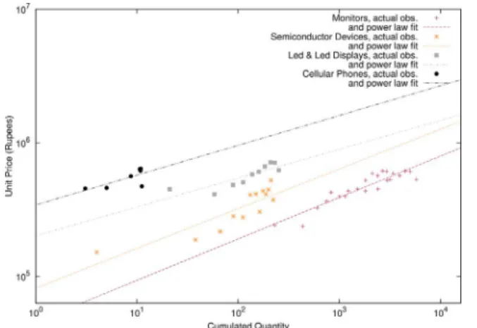
Fig. 2 illustrates the canonical cost-quantity curves for some se-lected products obtained by pooling together thefirms producing the same product, for some goods displaying a downward sloping cost-quantity curve. Dots with different symbols represent different pro-ducts. Each dot with the same symbol represents a pair of (log) cu-mulated quantity and (log of) price for a givenfirm in a given year. This evidence is well in line with several other studies that detect a cost-quantity relationship that is accounted for by a power-law and that applies to a wide variety of technologies (Dutton and Thomas, 1984; McDonald and Schrattenholzer, 2001; Argote and Epple, 1990). Con-versely, Fig. 3 offers a graphical account of some of the “positive” learning curves, that is, a positive relationship between unit price (or

Fig. 2. The relation between cost and quantity (log scale) together with power lawfit for selected products; the‘canonical’ downward sloping learning curves.

Fig. 3. The relation between cost and quantity (log scale) together with power lawfit for selected products; the upward sloping learning curves.

Fig. 4. Learning along the cost curve of one product vs learning to produce new products.

11_{Koh and Magee (2006, 2008)claim that an exponential function of time predicts the}

performance of several different technologies. According toGoddard (1982)costs follow a power law in production rates rather than cumulative production. Multivariate forms involving combinations of production rate, cumulative production, or time have been examined bySinclair et al. (2000)andNordhaus (2014).

12_{Since we are comparing log vis-à-vis non-log models, we also perform the following}

additional check. We take the exponential of the predicted values for the exponential and power model, then we compute the R2_{as the difference between (exponential of) the}

observed and predicted values. Note that the average R2_{hence obtained is 0.4, which is}

comparable to values from OLS estimation of the linear models. Nevertheless, the R2_of

the non-linear models are still higher than the linear models.

13_{The mean, standard deviation, skewness and kurtosis of the distribution are−1.60,}

cost) and experience.

The evidence so far shows that, in most of the cases, the cost-quantity relationship displays a non-linear nature and that such re-lationship differs across products, even in terms of sign. In the following section we look at the heterogeneity in learning patterns across pro-ducts andfirms, classifying them on the basis of the different techno-logical intensities, as captured by the Pavitt taxonomy (Pavitt, 1984).

5. Heterogeneity in cost-quantity relationships

Let us try to investigate the differences in cost-quantity relation-ships, conditional on the sectors the products belong to.

There could be various product-specific characteristics which might lead to the observed differences in learning patterns. Here, we are in-terested to investigate the technological characteristics of the product. Our hypothesis is that the products which show a positive relationship between cost and experience undergo systematic quality upgrading over time, hence the observed positive cost-quantity relationship. The general idea is that there are two types of learning, namely one asso-ciated with an increased efficiency in the production of a given product and another one linked to the ability of producing new/improved pro-ducts. The case is illustrated inFig. 4with unit costs/prices on the y-axis and, for convenience, time on the x-y-axis (recalling that time and cumulated production are equivalent if production grows ex-ponentially).

In a world of pure“process” learning firms would simply go down the Product 1 curve starting from C1(t1) and following a canonical learning curve. Suppose however that at some point in time thefirms introduces “better” product with initial cost C2(t2) and begins to im-prove its production capabilities on it, until it introduces yet another improved product with initial cost C3(t3), etc. Any observer unable to distinguish“learning” along the curve vs. product innovation - as we are not - would actually observe an upward sloping (or for that matter flat) long-term relation between costs/prices on the one hand, and time/cumulated production on the other.14 Further, the problem is compounded by the inability to calculate some quality-weighted prices (i.e. proxies for“hedonic prices”).

These are all problems which we faced in Dosi (1984) when studying the semiconductor industry. In that case, the pace of both

product and process innovation has been (and is) so fast that Moore's law applies (see above).15

For most products and most technologies, however, this is not the case and the slopes and signs of the price/quantity relation is going to be shaped by the relative balance between product-innovation and pro-cess-related learning. In turn such a balance is going to depend also by the type of sector the products belong to. And here is where Pavitt Taxonomy comes in.

5.1. Sectoral characteristic and learning modes

Pavitt (1984)distinguishes between sectors and technologies ac-cording to sources of technological knowledge, requirements of the users, and appropriability regimes (Pavitt, 1984). He identifies four categories:

(1) Supplier-Dominated sectors which include most traditional activities such as textiles, clothing and agriculture and mainly rely on sources of innovation external to thefirm, often equipment-embodied. (2) Scale-Intensive sectors, characterized by scale-biased technical

ad-vances and covering both basic materials and consumer durables, e.g. automobiles. Sources of innovation are both internal and ex-ternal to thefirm and innovation, especially in complex product such as automobiles and consumer durables is related to both product and process.

(3) Specialized Suppliers design and produce industrial machinery and instruments used in most other industrial sectors. Innovation is mostly product-innovation.

(4) Science-based sectors, rely on both in-house R & D and on university research; they include industries such as pharmaceuticals and electronics. The rates of product innovation are generally quite high while improvement in production efficiency vary a lot across sec-tors (e.g. very high in the mentioned case of semiconducsec-tors; of lesser importance for pharmaceuticals).

In terms of Pavitt's taxonomy one would expect, other things being equal, a dominance of standard downward sloping learning curves in

Fig. 5. Distribution of learning coefficients across different Pavitt categories at firm-level. S-D– Supplier Dominated; S-I – Scale Intensive; S-S – Specialized Suppliers; S-B – Science-based.

Table 5

Heterogeneity of learning coefficients across different Pavitt sectors: Two Sample Fligner–Policello Robust Rank Order Test.

Sector Obs. Average placement Index of variability F-P statistic Two-tailed p-value Supplier-dominated 24156 2.4e+04 4.5e+12 5.654 0.000 Scale-Intensive 47207 1.2e+04 2.3e+12

Supplier-dominated 24156 6.7e+03 1.8e+11 17.648 0.000 Specialized suppliers 11870 1.1e+04 8.3e+11 Supplier-dominated 24156 4.9e+03 1.1e+11 33.693 0.000 Science-based 7858 9.0e+03 4.2e+11

Scale Intensive 47207 6.6e+03 3.4e+11 15.964 0.000 Specialized

Suppliers

11870 2.1e+04 3.2e+12

Scale Intensive 47207 4.8e+03 2.1e+11 31.946 0.000 Science-based 7858 1.8e+04 1.6e+12

Specialized suppliers

11870 4.2e+03 7.5e+10 9.236 0.000 Science-based 7858 5.5e+03 7.5e+10

14_{InAppendix B, we attempt to show graphically the price trends of few products}

where the change(s) in product design can be visually detected.

15_{A deeper challenge, as pointed out by a referee, concerns the‘elementary objects’, if}

any, to which learning applies. So for example, in the paradigmatic example of micro-processors, it is not that the cost of each‘unitary transistor’ on an Integrated Circuit or a microprocessor goes down. On the contrary, it is the overall cost of a multiplicative number of transistors on a single chip.

technologies/sectors where process learning prevails and a more blurred pictures in the other ones.

Fig. 5 shows the “violin plots” of the distributions of learning coefficients across different Pavitt categories. The plot is a combination of box plot and kernel density distributions. The median of the product-level learning coefficient for each sector is marked by the central bar and the box indicates the interquartile range as in standard box plots. Indeed the distribution of learning coefficients in the Science-Based and Specialized Suppliers category (S-B and S-S in the figure) is shifted upwards, implying that there are more cases of positively shaped cost-quantity curves, while most of the observed patterns among Supplier Dominated and Scale Intensive sectors presents negative coefficients (price/costs fall with cumulated quantities).

The difference between the learning parameters across Pavitt sectors is further tested using Fligner–Policello location test (Fligner and Policello, 1981). The null hypothesis for the test is H0:θX=θY, whereθX andθYare the population medians of two Pavitt sectors in each pair.16 The test assumes that the distribution in each class is symmetric around the class median, but it does not require that the two class distributions have the same form or that the class variances be equal.17Table 5reports the pairwise Fligner–Policello statistics of the distributions of learning coefficients across different Pavitt categories. A positive and significant F-P statistics suggests that the distribution of learning coefficients of the second sector in each pair (for instance, scale intensive sector in thefirst row) statistically dominates the other. In all the cases we observe that the “learning” coefficients in specialized suppliers and science-based sectors statistically dominate the supplier dominated and scale intensive sectors: that is, there is a higher probability to observe a positively shaped learning curve, i.e. an apparent“anti-learning”.

Interestingly, we alsofind that for multi-product firms, in 90 per-cent of the cases, all products produced by thefirm display similar cost-quantity trend. It is further circumstantial evidence of the influence of the nature of underlying technologies which thefirms masters on the sign of its‘learning’ coefficient. Given the existence of such inter-sec-toral differences, we next investigate the presence of firm-specific characteristics associated with such learning patterns.

6. Cost-quantity relationships andfirm characteristics: product vs process innovation

The main sector of activity of thefirms deeply influence the pro-pensity to undertake R & D and thus the balance between product and process innovation as R & D is to a large extent addressing product in-novation/imitation. Still inter-firm variability remains high. Thus, here we investigate the relation between firms’ R & D and investment spending to the observed learning patterns at thefirm-product-level.

We perform OLS regressions to investigate the relationship between the observed learning parameters and innovative activities, separately for each Pavitt group of sectors. The proxies we consider for innovative activities are log of cumulated R & D for product innovation and log of cumulated investment, possibly capturing capital-embodied, for process innovation.18

The estimated model is the following cross-sectional regression:

=α+β R D +β +

LPij 1 & i 2Invi controlsi (7)

where LPijis the estimated learning parameter for product j produced byfirm i, Inviis log of cumulated investment offirm i and R & Diis the log of cumulated R & D of firm i. The controls include firm size,

Table 6

Learning coefficients of products and innovative characteristics of firms in different Pavitt sectors.

Supplier dominated Scale intensive

I II III I II III R & D 0.0204*** _0.0193*** _0.0190*** _{R & D 0.0083}*** _0.0077** _0.0074** (0.0038) (0.0042) (0.0042) (0.0027) (0.0030) (0.0031) Investment −0.0147*** _−0.0181*** _−0.0172*** _{Investment −0.0319}*** _−0.0326*** _−0.0336*** (0.0023) (0.0036) (0.0038) (0.0030) (0.0034) (0.0034) Size No 0.0011 −0.0024 Size No 0.0017 0.0054 (0.0036) (0.0044) (0.0040) (0.0044)

Year dummies No No Yes Year dummies No No Yes

Sector dummies Yes Yes Yes Sector dummies Yes Yes Yes Observations 6235 5260 5260 Observations 11,659 11,659 11,659

R2 _{0.155 0.181 0.184 R}2 _{0.060 0.060 0.062}

Specialized suppliers Science based

I II III I II III R & D 0.0347*** _0.0397*** _0.0395*** _{R & D 0.0159}** _0.0314*** _0.0322*** (0.0063) (0.0075) (0.0076) (0.0080) (0.0083) (0.0082) Investment −0.0062** _−0.0216*** _−0.0221*** _{Investment 0.0230}*** _0.1144*** _0.1140*** (0.0028) (0.0051) (0.0051) (0.0057) (0.0073) (0.0072) Size No 0.0216*** _0.0209*** _{Size No −0.1384}*** _−0.1577*** (0.0060) (0.0061) (0.0078) (0.0080)

Year dummies No No Yes Year dummies No No Yes

Sector dummies Yes Yes Yes Sector dummies Yes Yes Yes Observations 6441 5166 5166 Observations 4814 3670 3670

R2 _{0.036 0.043 0.047 R}2 _{0.020 0.114 0.142}

Standard errors in parentheses. ** p≪ 0.05.

*** p≪ 0.01.

16_{Thefirst column ofTable 5gives different pairs of Pavitt sectors.}

17_{SeeHollander et al. (2014)andJuneau (2007)for details.}

18_{SeeBogliacino et al. (2012)for a detailed review of innovation, and in particular}

measured as log of sales, year and 2-digit sector dummies. In Eq.(7), RHS variables are at firm-level, since we observe the R & D and in-vestment spending atfirm-level, not disaggregated by single products. The LHS variable, i.e. the learning parameter, is computed at the firm-product-level, as in Eq.(6).

Table 6shows the regression results for all four Pavitt sectors.19The first row shows the coefficient values for R & D. In all the sectors, the coefficients are positive and significant suggesting that, even within the same Pavitt sector, higher spending on R & D is associated with higher values of the learning parameter, that is, higher probabilities to observe a positively shaped“learning curve”.20_{The higher spending on R & D in} turn suggests an underlying quality upgrade of the product over time, i.e. various forms of product improvement/innovation.

Concerning investment intensity, in three out of four Pavitt sectors, the coefficient is significant and negative, as one would expect on the grounds of capital embodied process innovation. This suggests that higher spending on investment is associated with faster improvements in production efficiency. Interestingly, this does not seem to apply to the Science-Based cluster, hinting at the possibility that here new in-vestments are primarily associated with the manufacturing of new products.21

The foregoing evidence adds against the notion that the only driver of technological learning is by‘collective experience’. As important as we deem it is (see, among the many others,Dosi et al., 2000), many other modes are there. Some are apparently orthogonal to experience: seeSinclair et al. (2000)andFunk and Magee (2015).22_Ourfindings here suggest an apparent, most likely spurious anti-correlation which appears in a catching-up country. As such it is a puzzle, but also it hints, at normative level, at the possible usefulness of‘infant industry’ mea-sure whenfirms walk up the ladder of product qualities.

7. Firm entry and learning in the market

Recall that the foregoing analysis regard product-level learning curves, generally involving unbalanced panels of diverse firms. The results therefore summarize also information about entry, the initial prices at whichfirms enter in any one product category – possibly with distinct product qualities, and the learning process thereafter. In terms of industrial dynamics, entry of course involves a challenge to the market position of the incumbents, while thereafter learning as such represents a barrier to entry as it establishes a cost differential between

incumbents and would be entrants over the same product quality. InDosi (1984), one sketches out a model of industrial evolution inspired by semiconductors, but as such might be applicable to a wide range of industries, both on the frontier and in the catching up phase– characterized by the co-existence of product innovation and product-specific learning-by-doing. The latter continuously induces advantages to incumbents, but that can be always overcome by introduction of new/improved products in the same family, but with improved func-tionalities. The prediction of the model is a persistent process of entry, jointly with subsequent learning-by-doing, and possibly with new/im-proved products.

Of course, on the grounds of our data we have no way of accessing the techno-economic features of each product, but a story of persistent late entry cum higher entry prices is consistent with such conjecture. This is what wefind indeed in the Indian case. At a finer level of re-solution, one would expect, on the grounds of a capability-based theory of thefirm (Dosi, 1982; Dosi et al., 2000; Teece and Pisano, 1994) that late entrants which however have learned in related products know also how to produce“better products” at lower costs from the start.

Table 7shows summary statistics onfirm-product entry prices with respect to the average price of the incumbents producing the same good, or in other words, the market price. Market price is defined as the weighted average price of the product at the market level (incumbents) where the weights are the physical quantities of sales of the product.23 Afirm-product entry might occur either when an existing firm adds a new product to its portfolio or in presence offirm entry, that is when a newfirm enters the dataset. Of course, as we are interested in assessing the performance of newfirm-product combinations relative to firms that are incumbent in that product-market, we restrict our attention to products for which there are at least 10 other competitors. Column 1 of Table 7shows the different product tenures, i.e., the number of years the incumbents are producing one product.24 _{Column 2 shows the} percentages offirm-product combinations where the firm-product entry occurs at a higher price than the market average. Column 3 shows the number of firm-product combinations where the firm-product entry price is lower than the market price. Column 4 shows the total ob-servations in each product tenure class. Column 5 shows the average of the difference (in logs) between weighted average market price and entrant price. We observe inTable 7that with increasing product te-nure, i.e., the higher the number of years the incumbents are producing

Table 7

Descriptive evidence offirm entry in a given product. Product tenure Higher price (%) Lower price (%) Observations Log-difference of price (Avg) 0–5 53.92 46.08 102 0.211 5–10 45.95 54.05 407 0.604 10–15 44.44 55.56 504 0.833 15–20 41.87 58.13 492 0.880 Table 8

Relation between“market experience” and firm entry pricing.

I II III IV V

Tenure 0.0617** _0.1228** _0.0923* _0.1470*** _0.1111**

(0.0285) (0.0514) (0.0531) (0.0542) (0.0559) Product Sales Share No No 0.0000 No 0.0000

(0.0004) (0.0004) Firm size No No −0.0026** _−0.0027**

(0.0009) (0.0010) Sector dummies No Yes Yes Yes Yes Time dummies No Yes Yes Yes Yes N 1867 1867 1561 1794 1501 (R2_{) 0.387 0.392 0.484 0.395 0.488}

Adjusted (R2_{) 0.088 0.072 0.163 0.062 0.154}

Standard errors in parentheses. * p≪ 0.10.

** p≪ 0.05. *** p≪ 0.01.

19_{We calculate clustered standard error in order to permit general heteroskedasticity}

and within-cluster error correlation.

20_{Indeed, as one would expect, Pavitt classes do not entirely explain R & D behaviour}

(or other aspects) of allfirms within the sectors and hence, heterogeneity of firms (also with respect to product innovation), within the Pavitt sectors is the norm.

21_{Note that such results do not change when the learning coefficients employed as}

dependent variable in the regression are computed including a proxy for previous ex-perience. Results are available upon requests.

22_{Other studies, which look at the functional performance metrics of products,}

em-ploying data on physical attributes or technological characteristics of the product also report evidence on improvement in the characteristics of products not necessarily related to production learning: see, among the others,Martino (1971),Brock (2006),Koh and

Magee (2006),Nordhaus (2007),Koh and Magee (2008).

23_{The average price is computed excluding the new entrant.}

24_{In order to precisely measure the tenure of the product, we drop the products that}

were present in thefirst year of our sample. For those products indeed, we have no in-formation about the actual year of introduction. Note however that in a robustness check in which we include all observations, results remain the same.

a product, the higher the difference between entrant and market price. In order to provide more detailed evidence, let us estimate the model:

= + + + +

+ +

P P α β β β

e

( / ) Tenure Product sales share Firm size year sector

j j j i

i

ij 1 2 ij 3 ij

ij (8)

where Pijis price of product j offirm i,Pjis the weighted average price of the product at the market level as defined before, Tenurej is the number of years the product has been produced by incumbentfirms and is our proxy for market experience or knowledge stock at the market level. We control for Product sales share, i.e., the share of sales of the product in total sales offirm in the year of entry and Firm size, measured as log of grossfixed assets of the firm and we include year and sector25 effects. Since we are looking at firm-product entry, a one-time event, we pool the entry events in different years together and hence there is no time dimension in our analysis, in this respect the year dummies allow to control for temporal effect. Therefore, we perform a cross sectional analysis and employ an ordinary least squares regression with product fixed effects. We calculate cluster-robust standard error that permit general heteroskedasticity and within-cluster error correlation.

The results are reported inTable 8and overall, they suggest that the higher the“age” of the product family, the higher is the ratio of entrant to market price. Hence, the result suggests that firms entering a new product market find more difficult to successfully engage in price competition, the longer is the tenure of the product on the market. Conversely, the size of the“product entrant” has a negative effect on the price-ratio.

8. Conclusions

Persistent technological and organizational learning is most likely the fundamental driver of economic dynamics since the Industrial Revolution and underlines all episodes of catching-up ever since (for pertinent discussions, seeFreeman, 1987; Cimoli et al., 2009). Learning takes various forms which the economics of innovation has investigated in detail (a critical survey is inDosi and Nelson, 2010).

One of such ways, is learning-by-doing, that is some relation between experience by making, usually proxied by cumulative production and increasing production efficiencies/falling cost and prices. It is im-portant to notice however that such statistical evidence does not ture only strict learning by experience. On the contrary, it partly cap-ture also those processes of capability accumulation, technological adoption, imitation, andfinally cumulative innovation, at the level of firms and sectors (more in Dosi and Nelson, 2010and in the case of Korean development, seeKim, 1999; Lee, 2013).

The evidence is quite robust, mostly collected so far on industries in developed economies. But does it properly apply also to developing ones? And what explains the inter-sectoral/inter-product differences in the apparent learning patterns, if any?

In this work, on Indian manufacturing, we do corroborate in a good deal of cases the power law relation of cost/prices vs cumulated pro-duced quantities. At the same time, wefind, first, a wide variation in learning coefficients which still demands satisfactory explanations. Second, relatedly, some relations appear to be positive, that is, an ap-parent“anti-learning”. Such patterns, however are consistent with some circumstantial evidence according to which learning tends to relate more to product than process innovation. Third, product innovation also explains why late entry in the same product family occurs notwith-standing learning curves, which as such represent entry barriers in fa-vour of incumbents.

Finally, note that our work, and more in general, the recent in-creasing availability of product level data, discloses new research tra-jectories that one only started to investigate here. For instance, in the development process, to what extent corporations are able to success-fully transfer specific production knowledge accumulated over the years in a given product to a different one? And, relatedly, within a firm, does one observe different learning patterns for products that compete in foreign markets vis à vis products sold only domestically? This is just part of the beginning of the opening-up of the black-box of catching-up learning. In turn, these endeavors ought to be considered as an essential part of the investigation of the microeconomics of cap-ability accumulation, as such an essential part of the dynamics of de-velopment.

Acknowledgements

We thank Martin Bell, Tommaso Ciarli, Alex Coad, Alessandro Nuvolari, Luciano Pietronero, Emanuele Pugliese, Gerald Silverberg, Andrea Zaccaria, and several participants at the 11th ENEF meeting in Manchester (2014), 15th ISS Conference in Jena (2014), 7th Asialics in Daegu (2014), 12th Globelics in Addis Ababa University (2014), the 9th EMAEE conference in Maastricht (2015), 13th Globelics conference in Havana (2015), the 2nd annual conference of the International Association of Applied Econometrics in Thessaloniki (2015), SPRU and LEM seminars for their insightful comments. We gratefully acknowl-edge the research support by the IBIMET-CNR (grant CrisisLab-ProCoPe) and European Union Horizon 2020 Research and Innovation programme under Grant Agreement No. 649186 - ISIGrowth. The usual disclaimers apply.

Appendix A. Data details

As mentioned in Section3, the data are from Prowess database, provided by the CMIE (Centre For Monitoring Indian Economy Pvt. Ltd.). Prowess is a database of active business entities for which information related to theirfinancial performance is available. By “active” business entities, CMIE means those business entities that are not mere registrations without any activity. By“business entities” CMIE implies that it is not restricted to only registered companies. Prowess do not cover the universe of active business entities, even though it is the largest and most comprehensive database on thefinancial performance of Indian business entities. The companies covered account for around 70 percent of industrial output, 75 percent of corporate taxes, and more than 95 percent of excise taxes collected by the Government of India. Earlier studies have used the same database at the firm-level, such asTopalova and Khandelwal (2011); Balakrishnan et al. (2000)andKrishna and Mitra (1998)to study the impact of reforms on productivity growth offirms andKumar and Aggarwal (2005)to study the the determinants of R & D behaviour and the impact of reforms on R & D behaviour.

Few studies already used the samefirm-product-level data. Among theseGoldberg et al. (2010a,b)study the relationship between declines in trade costs, the imports of intermediate inputs and domesticfirm product scope; whetherGoldberg et al. (2010a,b)focus on the characteristics of multi-productfirms and the link between product rationalization and trade reforms in India.

Below, we present some description on the product data used for the study.Table 2in the text reports summary statistics of product-reporting firms.

A.1 Product-level classification

All companies in the Prowess database are mapped to a product or a service in CMIE's standardized products and services classification. This mapping reflects the company's main economic activity during a year.26

The product and services classification developed by CMIE is based on the Indian Trade Classification (ITC) which, in turn is based on the Harmonized Commodity Description and Coding System, commonly known as the HS.27CMIE's standardized products and services classification has a hierarchical or tree-like structure in which each broad group, for instance, beverages or leather products is in turn split into narrower categories. At the end of this branching process onefinds the singular products.Table 9offers just an example of such hierarchical structure for the branches of beverages and leather products, the full classification is available through the data provider. Notice that, as it happens also with other comparable classifications of sectors and products, the highest level of detail might vary across different branches. In this respect, inGoldberg et al. (2010a,b)it is argued that the level of disaggregation provided in CMIE is just a variation in the product detail, such variation being a fundamental feature of sectors rather than emphasizing issues with the data. The Prowess database contains a total of 2411 products linked to 293five-digit NIC industries across 22 manufacturing sectors (two-digit NIC codes). Among these, we remove the products defined only at 2 digit, as they identify broad categories of products which might display a high degree of variability, whichfinally leaves us with 2281 products.

A.2 Matching from products to Pavitt sectors

The linking between the products and the NIC industries are provided by CMIE (the data providing company). The NIC follows the United Nation's International Standard Industry Classification (ISIC). As such, NIC 2008 classification has a one-to-one correspondence to ISIC Rev. 4 at 4-digit level. A detailed mapping of industrial activities to Pavitt sector is provided inDosi et al. (2008). The concordance from NAICS and ISIC Rev. 4 is based on the United Nation's concordancefile (available at the UNSTATS website).28

Appendix B. Evidence of changes in product design

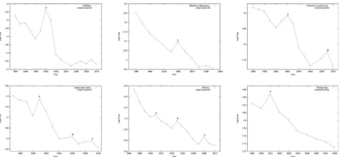
Here we attempt to show graphically the price trends of few products where the change(s) in product design can be visually detected.Fig. 6 shows learning curves for six products, where it is possible to detect a rather sharp trend in prices over a few years, which might be attributable to changes in product design. For example, thefirst plot on top-left ofFig. 6shows the price trend for the product CD/DVD, where we observe a sudden increase in price in the year 2000, probably because thefirm started producing DVDs instead of CDs, hence a change in the product characteristics.

Table 9

Example of the nested industry/product structure of Prowess. Source: Prowess database.

NIC Product code Description

11 products Manufacture of beverages

1103 Manufacture of malt liquors, beer and other

alcohol

050703010000 Malt spirit distilled 051401040000 Soda/Carbonated water

051403000000 Beer

051404010000 Sparkling wine

051406000000 Potable alcohol

051406010000 Indian made foreign liquor

051406010200 Heritage liquor

051406010300 Scotch & whiskey

15 products Manufacture of leather and leather products

1512 Manufacture of consumer goods of leather

and substitutes 070202040000 Shopping bags/carry bags

070202060000 Leather hand bag

070202070000 Wallets and leather purses 070203000000 Leather garments and accessories

070203010000 Leather jackets

070203020000 Leather gloves

070203040000 Leather belts

070203050000 Industrial leather hand gloves/apron 1520 products Manufacture of leather footwear

070601000000 Full leather shoes

070602000000 Canvas shoes

070603000000 Full shoes or boots

070604000000 Slippers

070605000000 Plastic footwear

070606000000 Footcare products

070607000000 Shoe uppers

070608000000 Shoe soles/heels

26_{A company is classified under a particular industry if more than half of its sales originates from the particular industry or industry group. The industry group could be any product or}

a product group in the CMIE products and services classification structure.

27_{The ITC system would only cover commodities but not services and utilities. However, CMIE has added them for its classification system.} 28_{The classification was lastly retrieved on March 2017 from:http://unstats.un.org/unsd/cr/registry/regot.asp?Lg=1.}

Appendix C. The proximate equivalence of Moore's law and Wright's law

Straightforwardly,“Moore's law” and “Wright's law” are equivalent if cumulated production grows exponentially over time: for some evidence, seeNagy et al. (2013). Moore's law can be formally expressed as

= −

p ( )a e βt ₍₉₎

where a is a constant (initial cost or price) and t is time. Moore's law here refers to the generalized statement that the cost or price of a given product decreases exponentially with time compared to Wright's law, which tests whether cost decreases at a rate that depends on cumulative production. In fact, empirically, there is a broad equivalence of Moore's and Wright's law. While comparing the Moore's parameter m (β in equation(9)) with the Wright's w (defined as −β from Eq.(6)in the main text of the paper), we observe a startling similarity between the two. The correlation between both the parameters is around 0.9 and the correlation between the R-squared of the two models is 0.95.

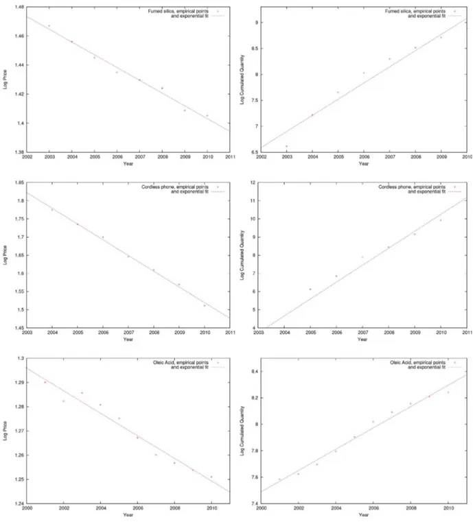
A straightforward explanation for the similarity has been highlighted bySahal (1979)showing that if the cumulative production, q, follows an exponential relationship with time, the Wright and Moore parameters are equivalent. Here, we check for the validity of Sahal's formulation and we start by verifying whether cumulative production, qt, follows an exponential function with time:

=

q_t a* exp(gt) ₍₁₀₎

We indeedfind that for all the products in our data, the cumulative production grows exponentially. The left column ofFig. 7shows three examples of products where production and price are plotted as a function of time.

The right column inFig. 7shows the trend of cumulative production in time. We observe that for the products for which the Moore's law is validated, also cumulative production grows exponentially in time.29

Eliminating t in Eq.(9)(Moore's) and Eq.(10), would result in Wright's law, withw=m g/ , where w is the Wright's parameter, m is the exponent of cost reduction (Moore's) and g is the exponent of the increase in cumulative production. We test this equivalence of Wright's and Moore's parameter inFig. 8by plotting Wright's parameter against m/g. The values cluster tightly along the identity line. These results are in line with the evidence inNagy et al. (2013).

While the equivalence of Wright's and Moore's parameter under exponential growth of output over time can be algebraically proven, the empirical question remains as to why that happens.Nordhaus (2014)tries to rationalize why production follows an exponential trend when cost decreases exponentially in time. He points out that when user-based performance of a product increases, or cost decreases, demand elasticity would result in an increase in demand (and thus production).

Fig. 6. Learning curves of selected products pointing to changes in product design.

29_{Notice that ourfindings should not be interpreted as a suggestion that cumulative production must grow exponentially with time in order for Moore's Law to hold. Till date, to our}

knowledge, the only work that could decouple time and effort variable (i.e., which finds cases where output does not follow an exponential increase with time) isMagee et al. (2016). Unfortunately, in this paper since for all the products we observe an exponential growth of cumulative production in time, we cannot test the alternative case.

Fig. 8. An illustration that the combination of exponentially increasing production and exponentially decreasing cost are equivalent to Wright's law. The value of the Wright parameter w is plotted against the prediction m/g based onSahal (1979), where m is the exponent of cost reduction (Moore's law) and g the exponent of the increase in cumulative production.