Generation of Pseudo-Random
Sequences for Noise Radar Applications
Gaspare Galati, Gabriele Pavan, Francesco De Palo Tor Vergata University – DIE and Centro “Vito Volterra”
Via del Politecnico, 1 – 00133 Rome, ITALY
[email protected] , [email protected] , [email protected]
Abstract — Noise Radar Technology (NRT) is nowadays a promising tool in radar systems. It is based on the transmission of waveforms composed of many noisy samples, which behave as LPI (Low Probability of Intercept) and antispoofing signals. Each noisy sequence is theoretically uncorrelated with the others. In the paper we propose a scheme to generate a “tailored” pseudo-random sequences (limited in amplitude). It will be followed by an analysis of the main performances in terms of the Peak Side Lobe Ratio (PSLR) of the autocorrelation function, cross-correlation analysis to evaluate the orthogonality, bandwidth and energy efficiency.
Keywords – Noise radar, low PSLR, orthogonal waveforms. I. INTRODUCTION
For the first time in 1959 the concept of noisy signal was introduced to implement a system able to measure the distance using a noise modulated signal [1]. During the ’60s - ’80s the research became more intense [2], [3], [4]. In the ’90s new methods for efficient generation of chaotic signals were developed in the millimeter band [5]. In the ’2000s several research groups have developed new applications for noise radar and made significant contributions towards detection, surveillance, tracking, and imaging of targets [6]. More elements about features, problems and potential of noise radar systems can be found in [7]. The progress of technology now offers the possibility to produce and process noisy waveforms. In fact, high-speed and high dynamic range Digital-to-Analog Converters (DACs) and high-speed large-scale Field Programmable Gate Arrays (FPGAs) facilitate generating high-performance precision digital waveforms. Moreover FPGAs and ADCs allow directly sampling of fairly wide bandwidth signals, and modern high speed processors allow more and more sophisticated filtering and detection algorithms to be employed.
The main advantage of noise radars waveforms is to achieve high resolution in both range and Doppler, which can be independently controlled by varying the bandwidth B and the integration time T respectively (the compression ratio BT is related to the number of independent samples to be process).
In general, one of the most important problem of the compression technique is the masking effect due to the presence of high sidelobes at the output of the correlation filter, i.e. weak echoes can be masked by the strong ones. In pulse and CW radars this problem is solved exploiting time and
frequency separation respectively. However in CW noise radars the noisy signal occupies the entire bandwidth at each instant of time, thus making impossible frequency separation and reducing radar sensitivity and detection range. Methods to solve masking effect can be conceptually divided in: (a) methods requiring extra signal processing at the receiver (for example the iterative algorithm known as CLEAN [8]) and (b) methods based on the waveform design with desired auto and cross correlation characteristics at the transmitter [9]. The main concept of (b) is filtering the noisy signal in the frequency domain with a window whose inverse Fourier Transform provides a low sidelobes level (low Peak Side Lobe Ratio). In the following a specific frequency window is used for the purpose to reducing the masking effect in transmitting section; it will be seen that a coherent azimuthal average of the outputs of the compression filter is necessary in order to achieve this goal. The waveforms design is one of the main focus of the research in modern radar systems, as MIMO (Multiple Input Multiple Output) radar [10] and Multifunction Radar [11], [12]. The MIMO and Multifunction radar applications require (in addition to the above mentioned low Peak Side Lobe Ratio) also good orthogonality properties (while maintaining the spectral occupancy into a limited bandwidth) and a low degradation in the main lobe (low Signal to Noise Ratio loss). Orthogonality may be imposed in time domain, in frequency domain or in signal space. Time division or frequency division multiplexing are simple approaches but they can suffer from potential performance degradation because the loss of coherence of the target response [15]. As a consequence, obtaining the orthogonality in signal space domain is the best choice, therefore this one will be considered in this paper. To obtain a low Signal to Noise Ratio loss an amplitude limiter (Zero-Memory-Non-Linearity transformation) will be used to maximize the transmitted power.
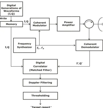
Fig. 1 presents a general architecture for coherent Noise Radar. The Digital Waveform Generator generates (I,Q) components of the transmitted noise signal which is stored in a memory and then modulated, amplified and transmitted. In the receiving section a coherent demodulator provides the base-band signal (I’,Q’); the output of the Digital Correlator is the output of the filter matched to the generated signal (I,Q).
The paper is organized as follows. Chapter II describes the generation method based on a filtering of a complex white Gaussian process followed by a Zero-Memory-Non-Linearity transformation to implement the hard or soft amplitude
IRS 2014, 15thInterna onal Radar Symposium, June 16-18, Gdansk, Poland
limitation. In Chapter III the criteria for settin the soft limiter will be analyzed with res orthogonality. Chapter IV contains som regarding the PSLR. Chapter V reports conc perspectives.
Figure 1. General architecture of a solid-state, co
II. WAVEFORMS DESIGN The proposed scheme to generate pairs signals is shown in Fig. 2. Starting from Gaussian noise and , the low-pa the goal of limiting the signal bandwidth autocorrelation function properties. The freq
the filter is obtained by w
Blackman-Nuttall spectrum, [16], has been c inverse Fourier Transform gives a functio sidelobes (order of ). The sample desidered spectrum for , are:
for , where are d
Figure 2. Block diagram to generate pairs of pseudo
ng the threshold of spect to loss and me considerations clusions and future
oherent, Noise Radar.
N
of pseudorandom m a pair of white ass filter has and defining the quency response of
where for a considered, whose on with very low es of , i.e. the
(1) defined in [16].
orandom sequences.
The block diagram in Fig. , represents the Di Fig.1; a pair and cross-correlation (i.e. to check The number of the gen sequence) depends on the bilat
and on the sampling freq
sequences and hav
constant amplitude. The la transmission power (meaning operating in saturation and the peak power). To reduce the Power Ratio:
has to be close to 1; this is o Non-Linearity (ZMNL) tran limitation may be either hard o
Given a complex signal the unit level) is obtained b keeping the phase of the (unit
soft limiter (see Fig. 3) the un
amplitude exceeds the threshol of the Rayleigh distribution; limiter case, while for remains in the linear zone. For is not limited.
Figure 3. Soft limiter charact
III. CHOICE OF TH The choice of the threshold characteristic of the transmitt variations of k produce limite shown in Fig. 4 for BT = 100 for k = 0 and k = 5, and in Fig 25 values of PSLR, for the com = 5000, 10000, 30000, 500 between the two cases ( a Considering the normalized 5 (dashed line) shows that a peak is almost constant vary difference is less than 1 dB correlation (for k = 0) results lo with the one of LFM up , i.e. -43 dB Linear
Sa
σ
. 2, considering a single signal igital Waveform Generator in
is generated to calculate the orthogonality).
nerated samples (for each teral band , on the pulse length quency . After filtering, the
ve limited bandwidth and non-atter causes “losses” in the
g that the transmitter is not average power is lower than the
loss, Mean Envelope to Peak
obtained using a
Zero-Memory-nsformation. This amplitude or soft.
, the hard limitation (to
by ,
t level) signal unchanged. For a nit level is reached if the input ld , where is the mode corresponds to the hard most input amplitude samples r example with , 99.97 %
teristic with threshold .
HE LIMITER THRESHOLD
d (parameter k) is driven by the ter amplifier. For a given BT, ed variations on the PSLR, as
00 considering two realizations g. 5 (continuous line) averaging mpression ratio BT varying (BT 000, 100000). The difference and ) is less than 1 dB.
cross-correlation function, Fig. also the mean cross-correlation ying k with assigned BT; the B. The minimum peak cross-ower than 14 dB circa compared
and down chirp, equal to B for BT = 10000 [17].
aturation
Figure 4. PSLR of a noise signal with hard limiter (k = 0) and witout amplitude limitation (k = 5).
Figure 5. Mean PSLR (continuous line) and mean Peak cross-correlation (dashed line), averaging 25 PSLR values, versus k, varying BT. The effect of the parameter on the spectrum is significant. Fig. 6 highlights the difference between the spectrum of an amplitude limited sequence, hard limiter ( ) and the one of the same limited sequence, soft limiter
( ).
Figure 6. Comparison between the spectrum obtained with hard limiter (k = 0) and soft limiter (k = 5).
In general the limiter, being a ZMNL device, causes the increase of the spectrum tails outside the band. This effect is stronger when is close to zero, while increasing , the limiter becomes similar to a linear characteristic mitigating the rise of the tails [18].
In many applications the minimization of the power loss in transmission may be an important requirement. The power loss can be written as function of the threshold :
Fig. 7 shows the power loss versus . For the amplifier works always in saturation (no loss). With a quasi linear characteristic, the loss is 10 ÷ 11 dB.
Figure 7. Loss of power versus the soft limiter parameter threshold (k). IV. PSLR AS FUNCTION OF THE COMPRESSION RATIO For random sequences filtered with a Blackman-Nuttall frequency window, the depends on the number of independent samples of the signal with an average
value of The signal has (i.e. the
compression ratio) samples only if it is sampled at sampling frequency . For example, if this is the case, a
theoretically produces sidelobes; however being the generated sequences (in according to the scheme of Fig. 2) realizations of a noisy random process, the of each autocorrelation is really 13 dB worse (i.e. greater) in comparison with the theoretical case.
Figure 8. Mean PSLR (with confidence interval of twice the standard deviation) versus BT (each value is obtained averaging 50 PSLR values).
-2 -1.5 -1 -0.5 0 0.5 1 1.5 2 -70 -60 -50 -40 -30 -20 -10 0 B = 50 MHz, T = 200 µs, BT = 10000 Time (µs) A u to c o rre la ti o n (d B ) k = 0, PSLR = -29.58 dB k = 5, PSLR = -29.06 dB 0 0.5 1 1.5 2 2.5 3 3.5 4 4.5 5 -40 -35 -30 -25 -20
Average: PSLR and Peak Cross-correlation, B = 50 MHz
k (d B ) BT = 5000 BT = 10000 BT = 30000 BT = 100000 BT = 50000 PSLR: continuous line Peak Cross: dashed line
-40 -30 -20 -10 0 10 20 30 40 -10 0 10 20 30 40 B = 50 MHz, T = 200 µs, BT = 10000 Frequency (Mhz) S p e c tr u m ( d B ) Hard Limiter, k = 0 Soft Limiter, k = 5 0 1 2 3 4 5 6 -12 -10 -8 -6 -4 -2 0 k P o w e r L o s s (d B ) 10.000 100.000 1.000.000 -55 -50 -45 -40 -35 -30 -25 -20 B = 50 MHz, Averaging 50 realizations PS L R ( d B ) BT k = 0 k = 5 -0.05 -0.025 0 0.025 0.05 -10 -5 0 117
Fig. 8 shows the mean (with confidence level of twice the standard deviation) versus , for and a threshold of and . The difference between the two cases is very small ( ).
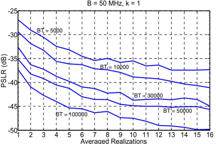
In order to reduce the PSLR, the outputs of the correlation receiver can be averaged coherently (if we consider each realizations referred to a single angular section, the average can be called “azimuthal”) obtaining an integration gain related with the number of averaged realizations, i.e. 12 dB averaging 16 realizations. Fig. 9 shows the PSLR improvement with respect to the averaged realizations.
Figure 9. PSLR versus the number of averaged outputs.
The improvemeny in PSLR level is significant, but the azimuthal average leads to a poor angular resolution. To avoid this issue you can still consider to use more than one realization for each angular direction with the use of a Pulsed (increasing the scanning time) or a Continuous Wave-MIMO radar (with orthogonal waveforms).
V. CONCLUSIONS AND FUTURE PERSPECTIVES A procedure for the generation of “tailored” pseudorandom signals has been proposed based on the use of a Low Pass Filter following by a soft limiter, whose threshold has been set equal to ( is the mode of the Rayleigh amplitude distribution). A soft limiter with showed a low power loss of only , while varying k the variations of the PSLR and the cross correlation are very limited (1 dB). Moreover, to improve the , it is appropriated to average coherently in
azimuth the outputs (8 or 16 realizations) of the correlation receiver.
REFERENCES
[1] B. M. Horton, Noise-modulated distance measuring systems, Proceedings of IRE, 49, 5 (May 1959), 821-828.
[2] C. D. McGillem, G. T. Cooper and W. B. Waltaman, An experimental random signal radar, Proceedings of the National Electronics Conference, Oct. 23, 1967, 409-411.
[3] M. Kaveh and G. T. Cooper, Average ambiguity function for a randomly staggered pulse sequence, IEEE Transactions on AES, AES-12, 3 (May 1976), 410-413.
[4] L. Guosui, G. Hong, S. Weimin, Development of random signal radars, IEEE Trans. AES, 1999, 35, (3), pp. 770–777.
[5] K. A. Lukin, Millimeter Noise Radar Technology, MSMW'98 Proc. Kharkov, Ukraine, September 15-1 7, 1998.
[6] D. Garmatyuk, M. Narayanan, Ultra-wideband continuous wave random noise Arc-SAR’, IEEE Trans. Geosci. Remote Sens., 2002, 40, (12), pp. 2543–2552.
[7] K. Kulpa, Signal Processing in Noise Waveform Radar, Artech House, 2013, ISBN: 978-1-60807-661-1.
[8] R. D. Fry, D. A. Gray, CLEAN deconvolution for sidelobe suppression in random noise radar, Proc. of the Int. Conf. Radar, 2-5 September 2008, Adelaide (Australia), pp. 209–212.
[9] G. Galati, G. Pavan, Orthogonal Waveforms for Multistatic and Multifunction Radar. Proc. of the 9th European Radar Conference,
Amsterdam 28 october 2 november 2012, pp. 310-313.
[10] Jian Li, P. Stoica, MIMO Radar Signal processing, John Wiley & Sons Inc., 2008.
[11] W. Benner, G. Torok., M. Batista-Carver, T. Lee, MPAR Program Overview and Status, Proc. of 23th Conference on International Interactive Information and Processing System (IIPS) for Meteorology, Oceanography and Hydrology, San Antonio (TX) 15-18 January 2007. [12] Federal Research and Development Joint Action Group for Phased
Array Radar Project (JAG/PARP) “Needs and Priorities for Phased Array Radar FCM-R25-2006”, June 2006.
[13] G. Galati, G. Pavan, Design Criteria for a Multifunction Phased Array Radar integrating Weather and Air Traffic Control Surveillance, Proc. EuRad 2009, pp. 294-297, Roma 30 September – 2 October 2009, Italy. [14] G. Galati, G. Pavan, On the Signal Design for
Multifunction/Multi-parameter Radar. Proc. of MRRSS-Microwaves, Radar and Remote Sensing Symposium 2011. Kiev (Ukraine), 25-27 August 2011, pp. 28-34, 2011.
[15] G. Galati, G. Pavan, S. Scopelliti, On range sidelobes suppression using frequency-diversity and complementary codes, Accepted by Transactions on Aerospace and Electronic Systems.
[16] H. Nuttall Albert, Some Windows with Very Good sidelobe Behavior IEEE Transactions on Acoustics Speech and Signal Processing, vol. ASSP-29, n. 1, pp. 84-91, February 1981.
[17] G. Galati, G. Pavan, Orthogonal and Complementary Radar Signals for Multichannel Applications. 8th European Radar Conference (EURAD)
Proceedings, pp. 178-181, 12-14 october 2011 Manchester (UK). [18] W. B. Davenport, W. L. Root, An Introduction to the Theory of Random
Signals and Noise, WILEY-INTERSCIENCE, 1987. 1 2 3 4 5 6 7 8 9 10 11 12 13 14 15 16 -50 -45 -40 -35 -30 -25 B = 50 MHz, k = 1 Averaged Realizations PS L R ( d B ) BT = 5000 BT = 10000 BT = 30000 BT = 50000 BT = 100000 118