Research Article
Development of an Indicator for the Assessment of Damage
Level in Rolling Element Bearings Based on Blind
Deconvolution Methods
Marco Buzzoni , Elia Soave, Gianluca D’Elia, Emiliano Mucchi , and Giorgio Dalpiaz
Department of Engineering, University of Ferrara, via Saragat 1, 44122 Ferrara, ItalyCorrespondence should be addressed to Marco Buzzoni; [email protected]
Received 23 May 2018; Revised 5 November 2018; Accepted 26 November 2018; Published 16 December 2018 Guest Editor: Emanuele Reccia
Copyright © 2018 Marco Buzzoni et al. This is an open access article distributed under the Creative Commons Attribution License, which permits unrestricted use, distribution, and reproduction in any medium, provided the original work is properly cited. The monitoring of rolling element bearings through vibration-based condition indicators plays a crucial role in the modern machinery. The kurtosis is a very efficient indicator being sensitive to impulsive components within the vibration signature that often are symptomatic of localized faults. In order to improve the diagnostic performance of the kurtosis, blind deconvolution algorithms can be exploited in order to detect bearing faults and, most importantly, their position. In this scenario, this paper focuses on the development of a novel condition indicator specifically designed for the damage as-sessment in rolling element bearings. The proposed indicator allows to track the bearing degradation process taking into account three different possible positions: outer race, inner race, and rolling element. This indicator fits real-time monitoring procedures allowing for the automatic detection and identification of the bearing fault. The validation of the proposed indicator has been carried out by means of both simulated signal and a run-to-failure experiment. The results highlight that the proposed indicator is able to detect more efficiently the fault occurrence and, most importantly, quicker than other established techniques.
1. Introduction
One of the most frequent failures in rotating machines is represented by bearing faults. The early detection and identification of bearing faults through vibration analysis is a powerful strategy in order to avoid or prevent catastrophic failures. However, the bearing fault identification can be very challenging since the impulsive pattern generated by peri-odic impacts due to localized faults is often masked by strong background noise, the dynamic response of the structure, and other mechanical interferences.
Over the years, several strategies have been proposed for the detection and identification of bearing faults. The most popular signal processing technique for bearing fault identification is the envelope analysis [1], but many other signal processing techniques have been proposed such as second-order cyclostationary analysis that involves for instance the cyclic modulation spectrum [2] and the spectral correlation [3], the spectral kurtosis [4], blind
deconvolution (BD) algorithms [5], and other advanced methods [6, 7].
Frequently, the final goal of condition monitoring is to condense a huge amount of information into a scalar number, also called condition indicator. The kurtosis, i.e., the fourth standardized moment, is probably the most used condition indicator for bearing diagnosis [8]. The success of kurtosis does not lie only in its effectiveness and computation simplicity but also in its relationship with the envelope analysis [9]. However, the kurtosis often fails because of strong interfering components [10–12], espe-cially if such masking contributions have impulsive na-ture. In this scenario, the BD methods can be used to reduce the stationary background noise and, in certain cases, to reduce the effect of masking contributions as well.
From a general standpoint, the goal of BD is to extract a source exhibiting a specific statistical property only from a noisy observation (response), under the hypothesis of a
Volume 2018, Article ID 5384358, 13 pages https://doi.org/10.1155/2018/5384358
linear time-invariant system. The term “only” refers to the fact that the system is assumed as unknown.
The first BD algorithm was introduced by Wiggins [13] in the field of seismic. Its methodology, called minimum entropy deconvolution (MED), blindly estimates an inverse filter which maximizes the kurtosis of the source. It should be noted that even if the name recalls the minimization of the entropy, MED is actually based on the maximization of the kurtosis. In other words, the MED extracts the source having the highest kurtosis. The main limit of this method in rotating machine diagnosis is that it tends to extract the most impulsive source rather than a pattern of periodic impulses; that is how the local faults of rotating machines appear in vibration signals.
The performances of MED in rotating machine diagnosis have been recently improved by means of two novel BD methods: maximum correlated kurtosis deconvolution (MCKD) [11] and multipoint optimal minimum entropy deconvolution (MOMEDA) [12]. Both methods are rooted on improved versions of the kurtosis criterion. The former has been proposed by McDonald et al. [11], and it is based on an improved version of kurtosis called correlated kurtosis (CK). The CK combines the maximization of the impul-siveness related with a certain repetition rate rather than only the maximum impulsiveness. The latter methodology has been proposed by McDonald and Zhao [12] and is based on a criterion called multipoint kurtosis (MK) which is a modified version of the kurtosis weighted by a Dirac comb which represents an ideal train of impulses generated by the expected fault. Both the BD methods proved to be effective for the fault identification in rotating machines, with par-ticular reference to gears and bearings.
Returning to the application of indicators for machine diagnosis, the final values of BD criteria can be exploited for assessing the bearing condition. In this direction, Sawalhi et al. [14] used the kurtosis values after performing MED in order to improve the sensitivity of kurtosis to the bearing faults. Analogously, McDonald et al. [11] exploited CK after performing MCKD together with a threshold for monitoring the condition of a multistage gearbox. Despite these promising applications [11, 14], the use of BD methods for monitoring the progressive damage of the system has not yet been exhaustively studied. Moreover, the use of the kurtosis and the MK involves some drawbacks. For instance, the kurtosis is not sensitive to the bearing fault position or the indicator variance can make their interpretation difficult.
The proposed research work focuses on the development of condition indicators for the bearing monitoring based on the framework of blind deconvolution methods. Such condition indicators can be synthesized in an online monitoring procedure which allows for automatically detecting and identifying the bearing faults through non-parametric thresholds. The core of this methodology is rooted on two novel indicators, called cumulative correlated kurtosis (CCK) and cumulative multipoint kurtosis (CMK) that are derived from CK and MK, respectively. These in-dicators overcome the kurtosis limitations since they allow for identifying the bearing fault being dependent on the characteristic fault frequency, and they are also robust to
impulse noise contributions. Moreover, the CCK and the CMK have two valuable properties for diagnostic purposes: as the sample size increases, their variance decreases, and they can keep track of the progressive damage of the bearing. This methodology is then particularly fit for industrial ap-plications which require clear data interpretation and early fault detection capability.
The proposed procedure is validated by using a simu-lated signal and a run-to-failure test provided by the Center of Intelligent Maintenance System (IMS) of the University of Cincinnati [15]. The results show that the CCK and the CMK overcome the performance of the raw values of CK and MK in terms of early fault detection and identification as well as bearing damage assessment. The results are presented and discussed in order to enlighten the improvements in-troduced by the proposed method.
Section 2 reviews the application of BD algorithms for bearing fault identification, with a specific focus on MCKD and MOMEDA. Section 3 addresses the new diagnostic method for the detection and identification of rolling ele-ments bearing faults through the definition of a novel condition indicator. Section 3 includes also a verification through a signal model. Section 4 concerns the experimental validation by using the IMS dataset. Finally, Section 5 summarizes the final remarks.
2. Bearing Fault Identification through Blind
Deconvolution Algorithms
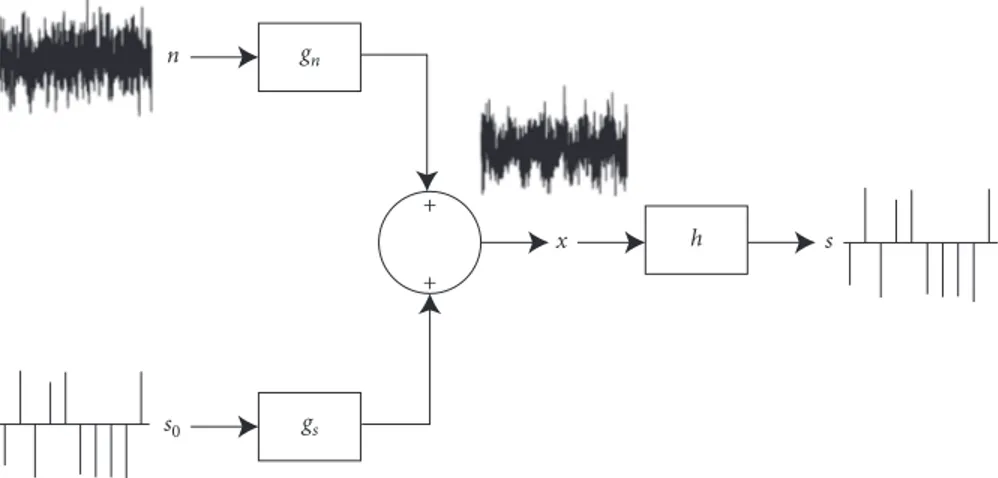
In general, the response due to a localized bearing fault occurring in a rotating machine can be modeled as a train of impulses convolved with an impulse response function (IRF) that characterizes the vibration transfer path between source and excitation. A scheme about how BD works on a sim-plified signal model is depicted in Figure 1.
The term “simplified” refers to the fact that the bearing fault signatures actually consist of a blend of random (cyclostationary) and periodic contributions [16], but, for the sake of simplicity, this formulation considers only the contribution of the transfer path and the background Gaussian noise. More details about how to model bearing fault signatures can be found in [17]. Figure 1 is a single-input-single-output (SISO) model that considers response x as a convolutive mixture of two contributions: (i) a repetitive train of impulses s0which refers to the excitation due to the
local fault and (ii) a Gaussian background noise n. Note that all these quantities are a function of time. Both are convolved with their respective IRFs depending on the system prop-erties (transmission path, natural frequencies, and damp-ing). The schematic in Figure 1 can be then formalized as follows:
x � s0∗ gs+ n∗ gn, (1)
where gsand gnare the IRFs related to s0and n, respectively,
and ∗ is the convolution operator. Frequently, gsand gnare
unknown, and the goal of BD methods is to estimate the inverse filter h, assumed to be a FIR filter that enables the extraction of s0 just through a noisy observation x.
The estimation of the source of interest, s0, can be
achieved considering an arbitrary criterion based on a prior assumption, e.g., assuming that a certain statistical property is strictly related to the target source. Therefore, the BD finds
h such that
s � x∗ h ≈ s0, (2)
where s is the estimation of s0by means of h. It is important
to underline that the approximation symbol refers to the fact that BD cannot recover the actual IRF but recovers the source, which exhibits the maximum value of the criterion. This research work focuses on two recent BD methods specifically designed for the diagnosis of rotating machines: the MCKD and the MOMEDA. Both criteria have been proposed considering the fact that a criterion which de-scribes the degree of impulsiveness of a vibration signal, e.g., the kurtosis, is often inadequate to deal with mechanical fault signatures. For instance, the vibration signature of a developed bearing fault is typically described by an im-pulsive contribution that is characterized by a series of impulsive components repeated according to the rotational frequency and the bearing kinematics. Thus, these criteria do not consider only the impulsive nature of bearing faults but also takes into account the repetition rate of this impulsive pattern. Thus, these criteria are particularly fit to detect bearing faults. A critical point shared by all the BD algo-rithms is the selection of the filter length. At the moment, it does not have any methodology or strategy for the filter length selection, and generally this choice relies on expe-rience and trial-and-error. However, it has been proved [5] that short filters could be not effective while long filters would lead to not acceptable computation times. From the author’s experience, a filter length between 50 and 200 samples is generally enough for obtaining satisfactory results.
2.1. Maximum Correlated Kurtosis Deconvolution. The
MCKD is an iterative BD algorithm that aims to extract the source having maximum CK. Unlike the kurtosis which measures the tailedness of a probability distribution and
reaches its maximum with signals having a dominant peak, the MCKD is sensitive to signal peakedness according to a given periodicity. The definition of CK is given in the following: CKM� Nn�1Mm�0sn−mT2 Nn�1s2 n M+1 , (3)
where T is the impulse period and M the number of shifts. The CK combines two features typical of the localized fault signatures, i.e., high kurtosis and repetitive occurrence of the fault. It should be noticed also that the CK is a cyclosta-tionary criterion. Indeed, the numerator of equation (3) with
M �1 is nothing but the autocorrelation function of the instantaneous power of the signal. In this particular case, the CK is a measure of the degree of autocorrelation referenced to a given lag T. Therefore, CK with M � 1 quantifies if the autocorrelation function exhibits periodicities at the fun-damental cyclic frequency 1/T. For this reason, the CK can be considered a cyclostationary criterion since a process which exhibits periodicities in its autocorrelation function is defined as a cyclostationary process.
It should be remarked that the CK [11] has been in-troduced empirically without explicit mention of its cyclostationary nature. By definition, the parameters of CK (i.e., the FIR filter length L and the number of shifts M) must be properly set in order to achieve satisfying results. In particular, M has to be carefully set if MCKD is applied to mechanical vibration signals. In fact, low values of M may not encourage enough the deconvolution of sequential impulses while high values of M, from experience more than 8, could lead to numerical precision issues since the CK can assume very low values.
2.2. Multipoint Optimal Minimum Entropy Deconvolution Adjusted. The MOMEDA is a noniterative BD method, and
it is an improvement of the OMEDA. In brief, the MOMEDA estimates a optimal inverse filter (in the least square sense) for recovering a source that approximates a target vector t, represented by a Dirac comb. The definition of the MOMEDA criterion is the following:
gn gs x h s s0 + + n
MK � 1 ‖t‖
tTs
‖s‖. (4)
Target vector t drives the deconvolution by imposing the spacing and the weights of the impulses to be recovered. Since t is defined as a train of equispaced impulses having unit amplitude, this criterion can be considered as a periodic one as opposed to the CK that is a cyclostationary criterion. Since it is a periodic criterion, it naturally fits with the diagnosis of gears or in any case of periodic fault signature. Indeed, its first application regards the identification of a chipped tooth in a 2-stage gearbox [12]. As said before, bearing fault signatures exhibit second-order cyclo-stationarity, and thus MCKD appears to be more suitable than MOMEDA for the fault detection and identification. However, a recent research [18] proved the effectiveness of MOMEDA for extracting bearing fault signatures taking into account the Case Western database.
3. Proposed Indicator and Diagnostic Protocol
3.1. Theoretical Formulation. The proposed method is basedon condition indicators, namely, CK and MK, capable to both detect and identify bearing faults at their early stage. Specifically, this research investigates how the final values of the criteria of MCKD and MOMEDA can be exploited as bearing condition indicators. Particular attention is devoted to verify how these indicators can be used for the real-time monitoring of bearings and for detecting trends related to the progressive degradation of the bearings.
Let ψ[k] be the final value of the BD criterion evaluated from a vibration signal in the time window k. Let us assume that ψ[k] is constituted of three different contributions: a constant (trend) part, a variable part, and a Gaussian noise. This model can be formalized as
ψ[k] � ψ[k] + ψ[k] + n[k], (5)
where ψ is the constant part of ψ, ψ is the variable part of ψ,
and n is the additive Gaussian noise.
Hypothesizing that the diagnostic information is retained into ψ, ψ and n de facto represent masking
con-tributions. Furthermore, variable part ψ is not supposed to
be necessarily a monotonically increasing function. This latter property is particularly useful for the design of robust indicators due to the fact that it allows for keeping trace of the “degree of damage” taking into account the whole time history of the component under investigation.
In order to reduce the effects of ψ and n, a possible strategy is to consider the cumulative of ψ:
c[j] �1
j
j
k�1
(ψ[k] + ψ[k] + n[k]), (6)
where index k refers to the kth signal segments while j refers to the total number of signal segments available. To give a real-life example of this kind of indexing, in an online condition monitoring system, k is the current measurement run while j is the overall number of measurements recorded. The selection of the number of segments to be considered is a
pivotal step for the proper estimation of the proposed in-dicator. In fact, the segment number should be selected carefully since a k too small would affect the consistency of the statistical threshold but a k too large would invalidate the hypothesis of healthy bearing in that time span. Generally, rolling element bearings are designed to work for a large number of cycles and therefore a time span of 1 day can be considered a reasonable trade-off.
Equation (6) is nothing but the sum of the expected values of all the contributions of ψ. After some simple manipulations, it can be noted that (under the hypothesis of large j) the estimated expected value of n converges to zero while the estimated expected value of ψ converges to its true (constant) value. Thus, equation (6) can be rewritten as follows: c[j] �E[ψ] +1 j j k�1 ψ[k], (7)
where E[·] stands for the expected value of ·. From the physical standpoint, the constant part of ψ, ψ, describes the healthy condition of the system, and the variable one, ψ,
reflects the occurrence of the bearing fault. At this point, after reducing the Gaussian noise contribution through the cumulative, the constant part ψ can be minimized as well by subtracting the expected value of ψ which is called E[ψ]∗:
β[j] � c[j] − E[ψ]∗�1 j j k�1 ψ[k], (8)
where E[ψ]∗is the expected value of data referenced to the healthy condition. E[ψ]∗ is theoretically unknown but a reasonable estimation can be done by estimating the mean value of ψ in the very first part of the acquisition when the component is supposed to be healthy.
Indicator β describes the evolution of the bearing con-dition and has two important properties: (i) it is mono-tonically increasing, so it retains all the variations in its whole time history, and (ii) it is consistent in the sense that the random noise is reduced according to the considered number of samples. This indicator can be therefore exploited for defining a diagnostic protocol in order to monitor bearings. Specifically, when β is close to 0, it means that the variable part of ψ is negligible and thus the system is healthy. When β changes, it means that the bearing condition is changing as well and an incipient bearing fault may be occurring. For this purpose, a nonparametric statistical threshold can be used, such as the thresholds evaluated through Tukey’s method [19]: mild outlier threshold TH,1
can be used for establishing when the bearing degradation process starts; outlier threshold TH,2 can be used for
establishing when the fault is manifest. Such thresholds are also called Tukey fences and can be calculated by means of the following formula:
TH� Q3+ p Q3− Q1, (9)
where Q3and Q1are the lower and upper quartiles while p is
a constant that defines TH,1if p � 1.5 and TH,2if p � 3. These
referenced to the first day of test, under the hypothesis that in this time span, the bearings are healthy. Note that a rule of thumb for bearing diagnosis is to discard the first hours of test since β may be affected by the contribution of running-in phenomena and consequently the related thresholds can be overestimated.
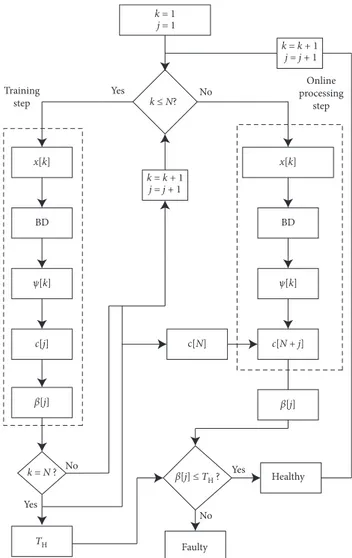
The proposed diagnostic protocol is reported schemat-ically in Figure 2 and can be summarized as follows:
(1) Training step: perform the BD algorithm on x[k], take the final value of the BD criterion (ψ[k]), compute the cumulative function c[j], and then subtract the expected value in order to obtain β[j]. Repeat this step for the N time spans referenced to the healthy condition in order to compute the thresholds TH.
(2) Online processing step: perform the BD algorithm on x[k], take ψ[k] and compute the cumulative function reduced by the expected value β[j]. (3) Compare the cumulative function β obtained in step
2 and the thresholds TH calculated in step 1. If β< TH, the bearing is healthy and the procedure
starts again from step 2. Otherwise, the bearing fault is detected and identified.
Note that in this paper, β will be called in two different ways: CCK and CMK.
3.2. Application to Simulated Data. Let us consider the signal
model described by equation (1). The reader should bear in mind that ψ can be any condition indicator estimated from a certain signal segment. For instance, we may decide to track the global vibration level of a component by monitoring ψ (e.g., CK or MK) value estimated each 1 s of measurement. A representation of this signal model having a total length of 20000 samples is reported in Figure 3 where Figure 3(a) refers to ψ, Figure 3(b) refers to ψ, Figure 3(c) is the additive noise, and Figure 3(d) refers to ψ.
The constant contribution is defined as
ψ[k] C, (10)
where C is constant and assumed as equal to unit while k is the sample index and must be integer and nonzero. The variable contribution is assumed to be composed of a si-nusoid with linear increasing mean:
n[k] 0, k≥ N∗, ψ[k] A sin 2π Lfk + mk, k ≥ N∗, (11) where the sine amplitude is A 0.1, the sine frequency is
f/L 2.5 · 10−4, and N∗ 2 · 104, while m 10−4 and
stands for the line slope. Finally, the background noise is modeled as a Gaussian distribution:
n[k] N(μ, σ), (12) where the mean is μ 0 while the standard deviation is
σ 0.1. The overall trend of Figure 3(d) shows a deviation
with respect to the previous constant trend after 10000 samples. However, the contribution that carries the di-agnostic information (i.e., ψ in Figure 3(b)) is strongly masked due to the presence of the noise as is clearly shown in Figure 3(d). Therefore, a trend close to the one shown in Figure 3(b) ( ψ) is desired for the assessment of the bearing damage level due to its easy interpretation. Moreover, if ψ is a monotonic increasing function, then the information provided would be even more valuable being actually a measure of the global degradation of the bearing that must be a quantity strictly increasing.
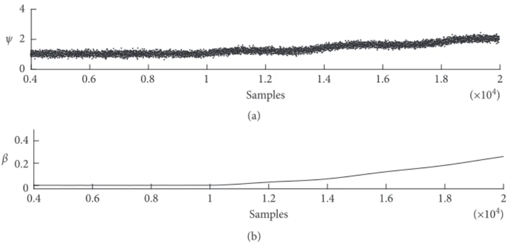
At this point, it is possible to compute β through equation (8) from the raw values of ψ. The results are reported in Figure 4 where Figure 4(a) reports the values of
ψ while Figure 4(b) reports the values of the proposed
indicator β. This numerical result shows that β actually exhibits the desired properties. Indeed, the variance of ψ has been significantly reduced and β is strictly increasing, in contrast with ψ that has an oscillatory behavior after 10000 samples. Moreover, β is also scaled with respect to a ref-erence value computed taking into account the first values of the time history. In machine diagnosis, this scaling allows for a better interpretation of the indicator
Yes No k = 1 j = 1 x[k] BD BD Yes No Faulty Healthy k = N ? Yes No TH x[k] k ≤ N? c[j] ψ[k] Training step Online processing step k = k + 1 j = j + 1 c[N] c[N + j] β[j] β[j] ≤ TH ? k = k + 1 j = j + 1 ψ[k] β[j]
since (approximately) nil values refer to healthy conditions and any deviation refers to anomalies in the system condition.
4. Experimental Verification
4.1. Setup. The data used in this experimental verification
have been provided by the Center of Intelligent Maintenance
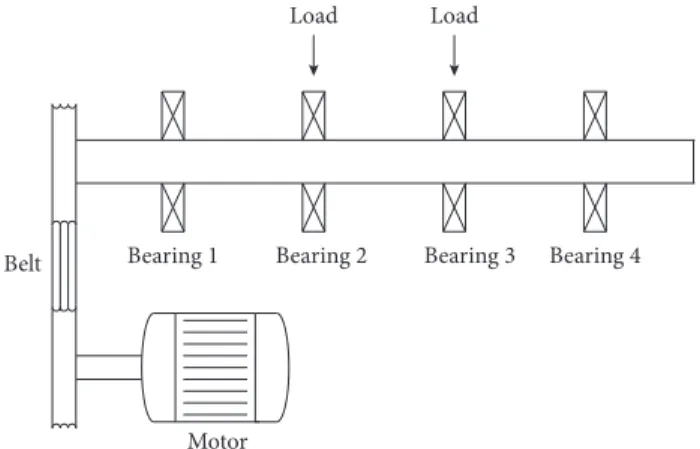
System (IMS) of the University of Cincinnati [15]. The test rig is composed of four bearings type Rexnord ZA-115 tied on the same shaft, as shown in Figure 5.
This test has been performed at constant speed of 2000 rpm with a load of 27.7 kN applied on bearings 2 and 3. The vibration signals have been collected by four ac-celerometers type PCB 253B33 mounted in radial di-rection. The vibration signals have been recorded with a
0 0.2 0.4 0.6 0.8 1 1.2 1.4 1.6 1.8 2 0 1 2 Samples, ψ ψ — (×104) (a) 0 0.2 0.4 0.6 0.8 1 1.2 1.4 1.6 1.8 2 0 1 2 ψ⌃ Samples, ψ (×104) (b) 0 0.2 0.4 0.6 0.8 1 1.2 1.4 1.6 1.8 2 –0.5 0 0.5 n Samples, ψ (×104) (c) 0 0.2 0.4 0.6 0.8 1 1.2 1.4 1.6 1.8 2 0 2 4 ψ Samples, ψ (×104) (d)
Figure 3: Simulated signal: (a) constant contribution ψ, (b) variable contribution ψ, (c) background noise, and (d) overall simulated signal ψ.
0.4 0.6 0.8 1 1.2 1.4 1.6 1.8 2 0 2 4 Samples (×104) ψ (a) 0.4 0.6 0.8 1 1.2 1.4 1.6 1.8 2 Samples 0 0.2 0.4 (×104) β (b)
Figure 4: Comparison of the trends of (a) the raw indicator ψ and (b) the proposed indicator β in the case of simulated signal reported in Figure 3.
sampling frequency of 20.48 kHz with a rate of 1 s of ac-quisition each 10 minutes. After 7 days, corresponding to 16.4 minutes of actual acquisition, the test has been stopped and an outer race fault, occurred in bearing 1, has been detected.
4.2. Results and Discussion. The experimental data have been
investigated by means of the BD algorithms described in Section 2, specifically MCKD and MOMEDA. The final values of the BD criteria, respectively, CK and MK, have been computed for signal segments of duration 1 s in order to monitor the progressive damage of the bearings during the endurance test. According to the technical report pro-vided by the experimenters, an outer race fault has occurred in bearing 1. Hence, only the accelerometer placed on bearing 1 has been considered.
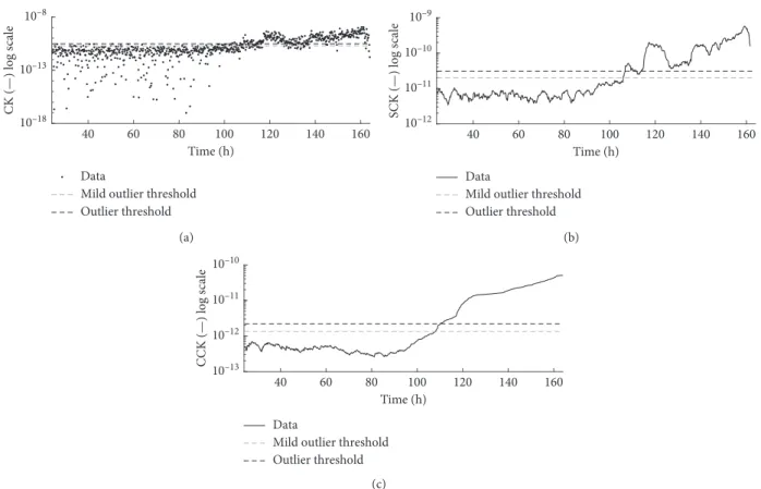
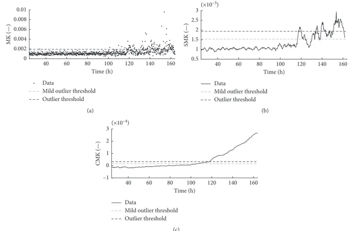
Figures 6 and 7 depict the application of the proposed methodology on the IMS dataset, respectively, by using the MCKD and MOMEDA analyses: Figures 6(a) and 7(a) represent the CK and MK values estimated for each signal segments of the endurance test, Figures 6(b) and 7(b) show the smoothed values of the previous CK and MK values, called for simplicity smoothed correlated kurtosis (SCK) and smoothed multipoint kurtosis (SMK), while Figures 6(c) and 7(c) report the values of the proposed indicator, namely CCK and CMK. All these figures include the nonparametric statistical thresholds, calculated as described in Section 3, in order to compare the time instant of the bearing fault appearance. Note that the SCK and the SMK have been computed by using the moving average technique and that these results are referenced to the prior period related to the outer race bearing fault.
Figures 6(a) and 7(a) clearly show that the trend of CK and MK is substantially constant taking into account in the first hundred hours of test. Reasonably, this behavior means that the bearings can be considered healthy in this time span. Then, the values change, according to the model given in equation (5): the variable part ψ is no
longer negligible with respect to the other contributions. Therefore, it can be noticed a time-dependent deviation with respect to the constant trend exhibited in the first
part of test. From the physical point of view, it can be deduced that this variation is directly related to the ap-pearance of a bearing fault. Moreover, the time-dependent variation of the indicators are not monotonically in-creasing but oscillatory. This fluctuating trend reflects the different stages of the bearing fault development and propagation which can be briefly summarized as con-secutive phases of damaging and healing until the com-plete breakdown. This mechanism of development and propagation of the bearing fault is reported and discussed in Reference [20].
In order to estimate the time instants associated to the fault appearance, the indicators must be compared with the thresholds calculated through Tukey’s method. Considering Figures 6(a) and 7(a), one can immediately find two drawbacks on the use of the raw BD criteria, hereafter called
ψ in general terms but referenced to CK and MK. The first
one is related to the dispersion of the values of ψ: although the major part of the values remains below the thresholds during the early stage of the test, some values cross the threshold although no fault has occurred. The second one regards the behavior of the variable part, ψ, during the last
stage of test: this variable contribution does not appear as a monotonically increasing function and thus the raw in-dicator ψ is not a good candidate for describing the bearing damage level since the bearing damage is conceptually irreversible.
The first issue, i.e., the variance of ψ, can be mitigated by using a smoothing technique, such as the moving average. This approach improves the results by reducing the dis-persion of the indicators, as reported in Figures 6(b) and 7(b). Indeed, the indicators (SCK and SMK) lie below the thresholds in the healthy stage but, during the faulty stage, are not able to represent the evolution of the fault with a strictly growing trend.
At this point, let us consider β defined in equation (8) as the absolute error between the expected value E[ψ]∗and the current value of the cumulative indicator c. By definition, β has two important properties: (i) its variance decreases when the number of observation increases and (ii) it is a strictly growing function in presence of nonnil values of ψ.
Figures 6(c) and 7(c) show the values of CCK and CMK estimated through the procedure depicted in Figure 2. As expected, CCK and CMK return a smoother trend with respect to the raw values of CK and MK (Figures 6(a) and 7(a)). At the same time, the dispersion is reduced further as well with respect to the smoothed values of CK and MK (Figures 6(b) and 7(b)). CCK and CMK show a strictly growing trend that makes the monitoring of bearing con-ditions and the fault detection easier, and it returns also consistent information about the overall damage level of the bearing. Therefore, this experimental verification demon-strates that β has a lower dispersion with respect to the raw indicator and that β is actually a monotonically growing function. These properties open to different scenarios concerning the industrial applications, in particular on the use of β as an indicator for the overall damage level of the bearing. Furthermore, the robustness of bearing fault de-tection through the combination of condition indicators and
Motor Bearing 1
Load
Belt Bearing 2 Bearing 3 Bearing 4
Load
thresholds is strongly improved thanks to the reduction of the data dispersion.
Figure 8 reports the time instants when the indicators cross threshold TH,1with reference to the results reported
in Figures 6 and 7. The experimental data used to validate the proposed diagnostics protocol do not provide the exact time instant in which the fault occurs, thus it is not possible to know exactly when the fault began. However, it should be noticed from Figure 5 that the test bench has been designed in order to permit the appearance of faults in the early stage of the test, due to the high radial loads applied on the bearings. Starting from this consideration, it is reasonable to think that for this particular application the indicator used for the analysis has to identify the ap-pearance of the fault, i.e., has to cross the thresholds, as early as possible. Considering the results related to the MCKD (first and second column of Figure 8), both SMK and CMK provide approximately the same time, specifi-cally 108 and 106 hours, respectively. This slight difference can be explained since MCKD is based on a cyclostationary criterion, and thus it is particularly suitable for the early fault detection of bearings. Considering the results related to the MOMEDA (third and fourth column of Figure 8), SMK and CMK provide values that are significantly dif-ferent, i.e., 116 and 105 hours, respectively. Comparing the times related to the CK and the MK (first and third column of Figure 8), it can be noticed a significant dif-ference in favor of the CK, due to the fact that the CK is
a cyclostationary indicator while MK is a periodic in-dicator. This difference is reduced if we consider the times referenced to the CCK and the CMK (second and fourth column of Figure 8). The reduction of the difference be-tween the time obtained by the application of the two different algorithms is strictly related to the earliest fault detection given by the CMK with respect to the raw values of MK. According to the previous consideration, this demonstrates that the proposed method is able to improve the effectiveness of the MK for the bearing fault detection in addition to its desired properties for the definition of a robust bearing damage indicator.
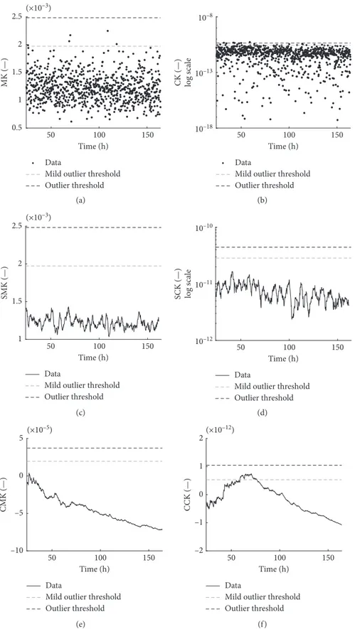
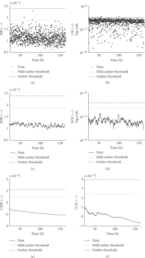
Until now, the analyses have been performed by using as a prior period the one referenced to the outer race fault. A further and necessary investigation is how the method be-haves taking into account also the other possible prior fault periods, i.e., the one related to the inner race fault and the one related to the ball bearing. The results of this other analysis, in terms of CMK and CCK trend, is summarized and shown in Figures 9 and 10.
According to what has been detected experimentally on the physical system, the only fault occurred on the bearing is the one on the outer race, thus the values obtained after the application of both BD algorithms should remain below the thresholds during all the test. It is possible to note in Figures 9(a), 9(b), 10(a), and 10(b) that due to the dis-persion of the values of BD criteria, some values cross the thresholds although no fault has occurred. After the
40 60 80 100 120 140 160 Time (h) 10–18 10–13 10–8 CK (—) log s cale Data
Mild outlier threshold Outlier threshold (a) 40 60 80 100 120 140 160 Time (h) 10–12 10–11 10–10 10–9 SCK (—) log s cale Data
Mild outlier threshold Outlier threshold (b) 40 60 80 100 120 140 160 Time (h) 10–13 10–12 10–11 10–10 C CK (—) log s ca le Data
Mild outlier threshold Outlier threshold
(c)
Figure 6: Application of the proposed method with MCKD: (a) CK values, (b) smoothed CK values (moving average), and (c) cumulative CK values. The considered prior period is referenced to the outer race bearing fault.
application of the smoothing technique, the obtained values lie below the thresholds during all the tests but their trends are not monotonic, as shown in Figures 9(c), 9(d), 10(c), and 10(d). Now, let us consider the values obtained after the application of the proposed diagnostic protocol, shown in Figures 9(e), 9(f), 10(e), and 10(f). It is possible to note that the trends of CMK and CCK for both prior periods, after a first stage, are decreasing; thus, the new condition indicators are able to describe the effective de-gree of damage of the system, according to the experi-mental observation. It is also worth noting that the CCK estimated by using the inner race fault frequency as a
reference prior period (Figure 9(f)) actually crosses the mild outlier threshold but just for a short time span and, above all, never crosses the outlier threshold.
5. Final Remarks
The kurtosis is widely recognized as a very efficient con-dition indicator being able to quantify the degree of peakiness of the vibration signature which is often related to fault occurrence. In this context, the kurtosis-based blind deconvolution (BD) techniques proved to be effec-tive for extracting the weak bearing fault signature from observations frequently plentiful of masking contribu-tions. In particular, the final values of the BD criterion can represent a convenient strategy for the assessment of the bearing condition. Despite some promising applications [11, 14], the use of BD methods for monitoring the pro-gressive damage of the system has not yet been exhaus-tively studied.
In this context, the proposed research work focuses on the development of a condition indicator rooted on BD methods and specifically designed for the assessment of the damage in rolling element bearings. The proposed indicator allows to track the bearing degradation process and to detect the bearing fault at its initial stage by means of a non-parametric statistical threshold. Specifically, the proposed indicators, i.e., CCK and CMK that are derived from the CK
106 108.3 116.5 105.5 SCK CCK SMK CMK Tim e (h)
Figure 8: Time associated to the appearance of the outer race bearing fault. 40 60 80 100 120 140 160 Time (h) 0 0.002 0.004 0.006 0.008 0.01 MK ( — ) Data
Mild outlier threshold Outlier threshold (a) 40 60 80 100 120 140 160 Time (h) 0.5 1 1.5 2 2.5 3 SMK ( — ) (×10–3) Data
Mild outlier threshold Outlier threshold (b) 40 60 80 100 120 140 160 Time (h) –1 0 1 2 3 CMK ( — ) (×10–4) Data
Mild outlier threshold Outlier threshold
(c)
Figure7: Application of the proposed method with MOMEDA: (a) MK values, (b) smoothed MK values (moving average), and (c) cumulative MK values. The considered prior period is referenced to the outer race bearing fault.
and MK, are sensitive to the fault frequency and keep track of the progressive damage of the bearing. Moreover, by definition, as the sample size increases, their variance
decreases. These aspects represent an improvement with respect to the other similar applications reported in Ref-erences [11, 14]. 50 100 150 Time (h) 0.5 1 1.5 2 2.5 MK (—) (×10–3) Data
Mild outlier threshold Outlier threshold (a) 50 100 150 Time (h) 10–18 10–13 10–8 CK (—) log s cale Data
Mild outlier threshold Outlier threshold (b) 50 100 150 Time (h) 1 1.5 2 2.5 SMK (—) (×10–3) Data
Mild outlier threshold Outlier threshold (c) 50 100 150 Time (h) 10–12 10–11 10–10 SCK (—) log s cale Data
Mild outlier threshold Outlier threshold (d) 50 100 150 Time (h) –10 –5 0 5 CMK (—) (×10–5) Data
Mild outlier threshold Outlier threshold (e) 50 100 150 Time (h) –2 –1 0 1 2 C CK (—) (×10–12) Data
Mild outlier threshold Outlier threshold
(f )
Figure 9: Application of the proposed method considering the inner race fault frequency starting from (a, c, e) MOMEDA and (b, d, f ) MCKD.
This methodology has been verified by means of a simulated signal and the IMS run-to-failure test by com-paring the diagnostic performance of the proposed indicator with respect to the raw values of the BD criteria. The results
show that the proposed methodology improves the effec-tiveness of the criteria of MCKD and MOMEDA for the bearing fault detection in terms of early fault diagnosis and clarity of data interpretation.
50 100 150 Time (h) 0.5 1 1.5 2 2.5 MK (—) (×10–3) Data
Mild outlier threshold Outlier threshold
(a)
Data
Mild outlier threshold Outlier threshold 50 100 150 Time (h) 10–18 10–13 10–8 CK (—) log s cale (b) 50 100 150 Time (h) 0.5 1 1.5 2 2.5 SMK (—) (×10–3) Data
Mild outlier threshold Outlier threshold (c) 50 100 150 Time (h) 10–12 10–11 10–10 SCK (—) log s cale Data
Mild outlier threshold Outlier threshold (d) 50 100 150 Time (h) –4 –2 0 2 4 CMK (—) (×10–4) Data
Mild outlier threshold Outlier threshold
(e)
Data
Mild outlier threshold Outlier threshold 50 100 150 Time (h) –1 0 1 2 3 4 C CK (—) (×10–12) (f )
Figure 10: Application of the proposed method considering the rolling element fault frequency starting from (a, c, e) MOMEDA and (b, d, f ) MCKD.
Abbreviations and Symbols
BD: Blind deconvolution
CCK: Cumulative correlated kurtosis CK: Correlated kurtosis
CMK: Cumulative multipoint kurtosis IRF: Impulse response function
MCKD: Maximum correlated kurtosis deconvolution MED: Minimum entropy deconvolution
MK: Multipoint kurtosis
MOMEDA: Multipoint optimal minimum entropy deconvolution adjusted
SCK: Smoothed correlated kurtosis SISO: Single-input-single-output SMK: Smoothed multipoint kurtosis
β: Proposed indicator
ψ: Constant part of ψ
ψ: Final value of the BD criterion
ψ: Variable part of ψ
c: Cumulative of ψ
g: Impulse response function
h: Estimated inverse filter
M: Number of shifts
n: Background noise
Qi: ith quartile s: Estimated source
s0: Source signal
T: Period of two consecutive impulses
t: Target vector
TH: Tukey’s threshold
x: Response signal.
Data Availability
The Matlab scripts used in this research are available from the corresponding author upon request. The vibration data used to support the findings of this study are freely downloadable at the following link: https://ti.arc.nasa.gov/ tech/dash/groups/pcoe/prognostic-data-repository/.
Conflicts of Interest
The authors declare that there are no conflicts of interest regarding the publication of this paper.
Acknowledgments
This research work has made use of data provided by the Center for Intelligent Maintenance Systems (IMS), Uni-versity of Cincinnati. The analyses have been performed through the Matlab code within the Minimum Entropy Deconvolution Multipack kindly coded and provided by Geoff McDonald.
References
[1] P. D. McFadden and J. D. Smith, “Vibration monitoring of rolling element bearings by the high-frequency resonance technique-a review,” Tribology International, vol. 17, pp. 3–10, 1984.
[2] G. Elia, M. Cocconcelli, E. Mucchi, and G. Dalpiaz, “Com-bining blind separation and cyclostationary techniques for monitoring distributed wear in gearbox rolling bearings,” in Proceedings of the Institution of Mechanical Engineers, Part C: Journal of Mechanical Engineering Science, vol. 231, 6, pp. 1113–1128, 2016.
[3] Z. Feng and F. Chu, “Cyclostationary analysis for gearbox and bearing fault diagnosis,” Shock and Vibration, vol. 2015, Article ID 542472, 12 pages, 2015.
[4] X. Zhang, J. Kang, L. Xiao, J. Zhao, and H. Teng, “A new improved Kurtogram and its application to bearing fault diagnosis,” Shock and Vibration, vol. 2015, Article ID 385412, 22 pages, 2015.
[5] M. Buzzoni, J. Antoni, and G. D’Elia, “Blind deconvolution based on cyclostationarity maximization and its application to fault identification,” Journal of Sound and Vibration, vol. 432, pp. 569–601, 2018.
[6] L. Cui, J. Huang, and F. Zhang, “Quantitative and localization diagnosis of a defective ball bearing based on vertical-horizontal synchronization signal analysis,” IEEE Trans-actions on Industrial Electronics, vol. 64, no. 11, pp. 8695– 8706, 2017.
[7] L. Song, H. Wang, and P. Chen, “Step-by-step fuzzy diagnosis method for equipment based on symptom extraction and trivalent logic fuzzy diagnosis theory,” IEEE Transactions on Fuzzy Systems, vol. 26, no. 6, pp. 3467–3478, 2018.
[8] R. B. Randall and J. Antoni, “Rolling element bearing diagnostics-A tutorial,” Mechanical Systems and Signal Pro-cessing, vol. 25, no. 2, pp. 485–520, 2011.
[9] P. Borghesani, “The envelope-based cyclic periodogram,” Mechanical Systems and Signal Processing, vol. 58-59, pp. 245–270, 2015.
[10] R. B. Randall, J. Antoni, and K. Gryllias, “Alternatives to kurtosis as an indicator of rolling element bearing faults,” in Proceedings of ISMA2016 International Conference on Noise and Vibration Engineering, pp. 2503–2516, KU Leuven, Leuven, Belgium, September 2016.
[11] G. L. McDonald, Q. Zhao, and M. J. Zuo, “Maximum cor-related Kurtosis deconvolution and application on gear tooth chip fault detection,” Mechanical Systems and Signal Pro-cessing, vol. 33, pp. 237–255, 2012.
[12] G. L. McDonald and Q. Zhao, “Multipoint optimal minimum entropy deconvolution and convolution fix: application to vibration fault detection,” Mechanical Systems and Signal Processing, vol. 82, pp. 461–477, 2017.
[13] R. A. Wiggins, “Minimum entropy deconvolution,” Geo-exploration, vol. 16, no. 1-2, pp. 21–35, 1978.
[14] N. Sawalhi, R. B. Randall, and H. Endo, “The enhancement of fault detection and diagnosis in rolling element bearings using minimum entropy deconvolution combined with spectral kurtosis,” Mechanical Systems and Signal Processing, vol. 21, no. 6, pp. 2616–2633, 2007.
[15] J. Lee, H. Qiu, G. Yu, and J. Lin, Rexnord Technical Services, Bearing Data Set, IMS, University of Cincinnati, NASA Ames Prognostics Data Repository, Cincinnati, OH, USA, 2007, http://ti.arc.nasa.gov/project/prognostic-data-repository. [16] J. Antoni, “Cyclic spectral analysis of rolling-element bearing
signals: facts and fictions,” Journal of Sound and Vibration, vol. 304, no. 3–5, pp. 497–529, 2007.
[17] G. D’Elia, M. Cocconcelli, and E. Mucchi, “An algorithm for the simulation of faulted bearings in non-stationary condi-tions,” Meccanica, vol. 53, no. 4-5, pp. 1147–1166, 2018. [18] Y. Wang, N. Hu, L. Hu, and Z. Cheng, “Rolling bearing fault
deconvolution adjusted technique and direct spectral analy-sis,” in Proceedings 2017 Prognostics and System Health Management Conference, PHM-Harbin 2017, Harbin, China, July 2017.
[19] F. N. David and J. W. Tukey, “Exploratoty data analysis,” Biometrics, vol. 33, no. 4, p. 768, 1977.
[20] T. Williams, X. Ribadeneira, S. Billington, and T. Kurfess, “Rolling element bearing diagnostics in run-to-failure lifetime testing,” Mechanical Systems and Signal Processing, vol. 15, pp. 979–993, 2001.
International Journal of
Aerospace
Engineering
Hindawi www.hindawi.com Volume 2018Robotics
Journal of Hindawi www.hindawi.com Volume 2018 Hindawi www.hindawi.com Volume 2018Active and Passive Electronic Components VLSI Design Hindawi www.hindawi.com Volume 2018 Hindawi www.hindawi.com Volume 2018
Shock and Vibration Hindawi
www.hindawi.com Volume 2018
Civil Engineering
Advances inAcoustics and VibrationAdvances in
Hindawi
www.hindawi.com Volume 2018
Hindawi
www.hindawi.com Volume 2018
Electrical and Computer Engineering Journal of Advances in OptoElectronics Hindawi www.hindawi.com Volume 2018
Hindawi Publishing Corporation
http://www.hindawi.com Volume 2013 Hindawi www.hindawi.com
The Scientific
World Journal
Volume 2018 Control Science and Engineering Journal of Hindawi www.hindawi.com Volume 2018 Hindawi www.hindawi.com Journal ofEngineering
Volume 2018Sensors
Journal of Hindawi www.hindawi.com Volume 2018 Machinery Hindawi www.hindawi.com Volume 2018 Modelling & Simulation in Engineering Hindawi www.hindawi.com Volume 2018 Hindawi www.hindawi.com Volume 2018 Chemical EngineeringInternational Journal of Antennas and
Propagation International Journal of Hindawi www.hindawi.com Volume 2018 Hindawi www.hindawi.com Volume 2018 Navigation and Observation International Journal of Hindawi www.hindawi.com Volume 2018