5
Traditional and Alternative Risk:
Application to Hedge Fund Returns
Claudio Boido1, Antonio Fasano2*1 University of Rome LUISS and Siena Via Banchi di Sotto, 55 - 53100 Siena
2 University of Rome LUISS and Salerno Viale Romania, 32 - 00197 Roma
Abstract: This study compares the risk-adjusted performance of traditional and alternative investments. Instrumental to this design, we introduce a specific metric for assessing hedge fund performance, comprising both the relative advantage and the extra-risk of an alternative investment over a traditional one. We are concerned with the impact of the crisis. Common wisdom tells us that during phases of market euphoria, investors’ wishful thinking can make them overconfident of the high returns promised by the leveraged structures and the aggressive investment policies typical of this asset class; conversely, when the downturns hit, the “big bets”, taken by hedge fund managers, in risky and illiquid investments, can trigger severe losses in their investors’ portfolios. We found evidence that regime switches in stock returns emphasise the performance gap among the different fund investment policies; furthermore, some styles can effectively capitalise on managerial skill, outperforming traditional equity investment in terms of adjusted performance.
Keywords: alternative investment, hedge fund, performace, risk measure JEL codes: G11, G12, G23
Part I
Introduction
1A hedge fund is an investment that offers risk and return opportunities not easily obtained with any other asset class. A hedge fund is an alternative asset class, that is, an asset class other than stocks, bonds, and cash2, where asset managers disclose only the main outlines of their strategy without going into technical details so as to keep their potential profits. If the financial markets are not efficient, active managers are able to beat markets to make a profit from their strategy. Each hedge fund follows a different strategy in terms of risk/return. These strategies reflect the individual manager’s skill and the performances are not linked to the benchmarks as
* Corresponding author
1 This study is a collaborative effort. Anyway, we can attribute Part I to Claudio Boido and Part II to Antonio Fasano.
2 Other notable forms of alternative investments include commodities, precious metals, real estate funds, and art.
mutual funds. The heavy use of leverage can have a potential effect on expected returns in terms of volatility even if in some strategies, as market neutral, the volatility tends to be lower. Therefore, hedge fund returns combine a manager’s skill and the features of the selected strategy which have shown a stronger correlation with equity markets than others over the year. Most investors classify hedge funds as alternative assets even if, during the fall of financial markets of 2008, the correlation between hedge fund indexes and equity indexes was approximately 0.82, that is, the hedge fund strategies had a bad impact on the financial crisis as well as on traditional asset classes. The explanation lies in the fact that the performance of each strategy is based on the exposure to the asset classes traded on the different markets, that is, when there is a market crisis, the same crisis is reflected in hedge fund returns. Billio et al. 2010 noted that there was an apparent interconnectedness among hedge funds, banks, brokers, and insurance companies during the financial crisis of 2007-2009, which amplified shocks into systemic events. Their results suggested that while hedge funds can provide early indications of market dislocations, they may not give significant contributions to systemic risk as those of banks, insurance companies and brokers. According to Eureka hedge publications, the assets managed by the hedge fund industry declined by $470 billion between June 2008 and April 2009. Fortunately, the flight of investors from the hedge fund industry stopped in May 2009, when inflows into the hedge fund industry exceeded outflows for the first time since June 2008. Given the shock experienced by the industry in 2008, it is certainly interesting to understand if and how the financial crisis altered the determinants of the flows experienced by hedge funds. In the first quarter of 2010, hedge fund– related trading accounted for almost one–third of the average U.S. daily share volume (Harris 2010). In 1990, according to estimates from International Financial Services (2010), some 530 hedge funds managed about $50 billion in assets; by the end of 2009, more than 8,000 hedge funds managed $1.6 trillion. The strategy mix of the hedge fund industry has also changed. In 1990, the industry was dominated by funds that followed a global macro strategy; in 2008, a sizeable majority of funds followed equity based strategies, such as long–short equity and event-driven approaches. As the events of 2008 have demonstrated, a large part of the average hedge fund beta boils down to straight equity and credit risk. In addition, particularly during the 1990s, the alternative part in hedge fund beta was passed off as absolute return (or alpha), which unreasonably cast a favourable light on the entire hedge fund sector. The growth of hedge funds in the last decade is justified by the following reasons. The first is the unprecedented wealth creation during periods of strong performance in the equity markets, which significantly expanded the base of wealthy private investors. Secondly, institutional investors, together with high-net-worth individuals, started showing greater interest in the hedge fund market. Thirdly, there was a need for effective instruments for diversification during periods of falling equity and bond markets. A “stable absolute return” during periods of different market conditions became more and more a target for both private and institutional investors. Indeed, hedge funds have less restriction on the use of constraints as leverage, short selling, and derivatives than more regulated vehicles such as mutual funds.
7
1 Taxonomy of Hedge Fund Strategies and Related Literature
There is not yet a large consensus on a unique classification of the hedge funds. Many researchers follow the strategy class and the specific strategy used by main large index providers (Hedge Fund Research, CSFB/Tremont, MSCI and Standard & Poor). There are at least eight distinct styles or philosophies of asset management currently employed by hedge funds, and risk exposure depends very much on style affiliation. It can be classified according to a systematic (strategies based on computer program) or a discretionary (strategies based on the opinion and sentiment of the fund managers) approach. Others classify hedge funds according to their geographical location, using this term in a different meaning of Fung and Hsieh, Fung and Hsieh (1997a), that is, in a more traditional meaning (Euro area, Emerging markets, U.S and U.K. markets). The large opportunity to classify hedge fund strategies also allows taking into consideration multi-strategies, when it is difficult to understand the risk/return relationship with a unique strategy.
The following classification was used by Eichengreen and Mathieson (1998) and there are 8 categories of hedge funds with 7 differentiated styles and a fund-of-funds category.
• Event driven funds. These are funds that take positions on corporate events,
taking an arbitraged position when companies are undergoing re-structuring or mergers. For example, hedge funds would purchase bank debt or high yield corporate bonds of companies undergoing re-organization (often referred to as ’distressed securities’). Another event-driven strategy is merger arbitrage. These funds seize the opportunity to invest just after a takeover has been announced. They purchase the shares of the target companies and short-sell the shares of the acquiring companies. Occasionally, they do the opposite if the deal is likely to fail.
• Global funds are a catch-all category of funds that invest in non-US stocks and
bonds with no specific strategy reference. It has the largest number of hedge funds. It includes funds that specialise in the emerging markets
• Global/Macro funds refer to funds that rely on macroeconomic analysis to bet on
major risk factors, such as currencies, interest rates, stock indices and commodities.
• Market neutral funds refer to funds that bet on relative price movements using
strategies such as long-short equity, stock index arbitrage, convertible bond arbitrage, and fixed income arbitrage. Long-short equity funds use the strategy of Jones by taking long positions in selective stocks and going short on other stocks to limit their exposure to the stock market. Stock index arbitrage funds trade on the spread between index futures contracts and the underlying basket of equities. Convertible bond arbitrage funds typically capitalize on the embedded option in these bonds by purchasing them and shorting the equities. Fixed income arbitrage bet on the convergence of prices of bonds from the same issuer but with different maturities over time. This is the second largest grouping of hedge funds after the Global category.
they may focus on technology stocks if these are over-priced and rotate across to other sectors.
• Short-sellers focus on engineering short positions in stocks with or without
matching long positions. They play on markets that have raised too fast and on mean reversion strategies.
• Long-only funds take long equity positions typically with leverage. Emerging
market funds that do not have short-selling opportunities also fall under this category.
• Fund of funds refer to funds that invest in a pool of hedge funds. They specialize
in identifying fund managers with good performance and rely on their good industry relationships to gain entry into hedge funds with good track records. On a risk-adjusted basis (dividing the mean return by the standard deviation), the category of fund that ranks highest is the market neutral funds followed by event-driven funds.
This classification is based only on self identification and it does not consider the risk and return profile of each hedge fund.
Many researchers have proposed different kinds of classification of hedge fund strategies, seeking to understand the guidelines of their investments.
Fung and Hsieh (1997b) classified hedge fund strategies following “style” (that is, the type of position the fund manager is taking) and “location” (that is, the asset class where hedge funds invest, for example equity, fixed income, commodities, currencies). Amenc and Martellini (2003) proposed a distinction between “return enhancer” and “risk reducer strategies”. In the first group we find hedge funds which seek higher expected returns but, according to the portfolio selection, they increase the volatility (that is, distressed securities, event driven, macro funds). In the second group active fund managers want to obtain positive excess returns reducing portfolio volatility (that is, convertible arbitrage, fixed income arbitrage, long/short and short selling funds).
In literature we can find some researchers who attempt to explain hedge fund returns on the type of asset classes and the styles of hedge fund managers.
Schneeweis et al. (1996) used a large set of indicators (returns, volatility by equity index, interest rates, exchange rates, commodity prices and future contracts) to show that hedge funds depend on different sets of factors compared to traditional asset classes (bond and equity). The same method is applied by Martin (2001), according hedge funds to a specific strategy through a cluster analysis. He used a regression analysis to ascertain a link between the performance of the different strategies and the selected economic factors. His results showed that a significant correlation exists when each strategy is pooled as an index.
Brown and Goetzmann (2001) examined the risk/return relationship of each hedge fund strategy cluster and so they used a cluster analysis algorithm to identify hedge fund strategy groups through a likelihood based ratio test to identify the optimal number of groups.
9 Asset allocation management style3, developed by Sharpe (1992), shows some problems in its application to hedge funds returns:
• It’s not clear which the right market indices as explanatory variables are. • Hedge fund managers use dynamic strategies, so the standard regression model
is not valid because asset exposures change quickly.
• Sharpe’s coefficient restrictions are not adequate for hedge funds, that is, leverage and derivative allow the exposures to go over the limit.
Agarwal and Naik (2000) inserted, as explanatory variables, options to improve the non-linearity in returns. Authors associate location, trading strategies and leverage, identifying the sources of returns (as Fung and Hsieh, 1997 and 1997b). A similar approach is adopted by Mitchell and Pulvino (2001) who ran a regression of returns on an equity market index. Brown and Goetzmann (2001) found that a difference in investment style explains about 20% of the cross sectional variability in hedge fund performance and they confirmed that the Sharpe model is used to measure exposure to investment management style. In a more recent study, Bali et al. (2011), Gregoriou and Pascalau (2012) argued that funds of hedge funds are, in general, over-diversified.
Shawky et al. (2012) investigated a significant relationship between diversification and performance and they found a considerable positive relationship across sectors and asset classes, while diversification across styles and location showed a significant negative association with hedge fund returns.
Even before the financial crisis, as written by Brown et al. (1999), Liang (2000), Agarwal and Naik (2000), and Kosowski et al. (2007), the failure risk in the hedge fund industry is high and rather persistent. Moreover, Kim (2008) examined failure risk in the hedge fund industry and found that hedge funds and funds of hedge funds fail as poor performance over an extended period of time (typically six to nine months) leads to significant withdrawals by investors. Cao et al. (2011) showed that hedge funds adjust their market exposure in the light of changing market liquidity, which potentially also affects their returns. Moreover, Sadka (2010) documented that unexpected changes in stock market liquidity are a priced risk factor in the cross-section of hedge fund return.
Finally, Boyson et al. (2010) found that large declines in stock market liquidity can be contagious to hedge fund returns. Mancini et al. (2011) showed that foreign exchange liquidity decreased significantly during the 2007–2009 period and that FX liquidity is correlated with measures of equity liquidity. A number of papers have argued that hedge funds that restrict investor liquidity perform better than hedge funds that do not restrict investor liquidity, including Schneeweis et al. (2002), Aragon (2007), Derman (2007), Aragon et al. (2008), Ding et al. (2009), and
3 This is a special application of regression analysis of fund returns, where the explanatory variables are returns on a set of market indices. It states that the regression coefficient is non negative and the sum of the coefficients must add up to one. In this way the coefficient on all markets indices can be understood as the percentage of the portfolio selected to that asset class.
Agarwal et al. (2009).
Although there is some evidence that hedge funds that restrict investor liquidity did better during an earlier time period (1994–2001), this result completely disappears during a more recent time period (2002–2009) and does not hold for the 1994–2009 sample period as a whole.
The literature on hedge funds characteristics is too large to be covered in detail here. The consensus so far is that the following hedge fund characteristics are related to performance.
• Size, cf. Harri and Brorsen (2004), Getmansky (2004), Ammann and Moerth (2005).
• Age, cf. Howell (2001), Amenc and Martellini (2003).
• Managerial incentives, measured using fee structure, cf. Ackermann et al. (1999), Liang (1999), Edwards and Caglayan (2001) or using delta Agarwal et al. (2009).
• Fund provisions, cf. Liang (1999), Agarwal et al. (2009).
• Past performance, cf. Agarwal and Naik (2000), Barès et al. (2003), Baquero et al. (2005), Jagannathan et al. (2010).
• Strategy, cf. Amenc and Martellini (2003), Brown and Goetzmann (2001). • Volatility, cf. Schneeweis and Spurgin (1998), Le Moigne and Savaria (2006). Many hedge fund indices have returns that are far from normally distributed, with negative skewness and a high kurtosis. In addition, many hedge funds claim that their return distributions are not normal due to the use of derivatives, short sales, and rebalancing rules. However, it is now well understood that hedge fund returns can be highly non-normal, which makes traditional performance measures, based on the assumption of normality, unsuitable.
Several researchers – Fung and Hsieh (1997a) and (1997b), Fung and Hsieh (2004), Mitchell and Pulvino (2001), Brooks and Kat (2002), Lamm Jr (2003), Agarwal and Naik (2004), Malkiel and Saha (2005), Eling and Schuhmacher (2007), Perelló (2007), Kat and Miffre (2008) - have shown the inadequacy of mean variance framework for measuring the performances of hedge fund portfolio, because it is valid only if the returns are normally distributed and that the distributions of returns are asymmetrical. Other authors, e. g. Bacmann and Pache (2003), Liang and Park (2007), Perelló (2007) have proposed using downside risk measure (Sortino ratio, Omega measure, Upside potential ratio4) as a solution to the asymmetry of returns to value the performance of hedge funds. As regards the newer approaches we can single out:
• Measures based on lower partial moments (Omega, Sortino, Kappa). • Measures based on drawdown (Calmar ratio, Sterling ratio, Burke ratio). • Measures based on value at risk (Excess return, Conditional Sharpe ratio,
4 We suggest to consult the original paper (Sortino and Price 1994 Sortino et al. 1999 Keating and Shadwick 2002)
11 • Modified Sharpe ratio).5
Some authors (Eling and Schuhmacher, 2007) conclude that the choice of performance measurement has no impact on the ranking of hedge funds and that the use of Sharpe ratio, based on the first two moments (i.e. mean and variance) provides an adequate description of the return distribution.
Part II
2 Empirical Analysis
2.1 Data Set and Methodology
A common inquiry for the hedge fund (henceforth HF) investor would be how these funds, as an alternative investment, compare with a traditional equity investment. Therefore, we will first analyse inter-style performance to identify the possible different style-dynamics, and subsequently we will risk-adjust this performance and designing an ad hoc alternative risk adjusted measure. By doing so, we will try to answer the question concerning whether the risks taken and subsequent results are randomly drawn or they can be considered the effect of a systematic and disciplined management policy.
The performance variability among fund groups, expressing the different managers’ investment policies and also proxying their skills, can be measured by means of F-tests, where one assumes as the null-hypothesis that the groups are indistinguishable on average.
Our dataset is comprised of a sample of funds over the period January 2006– December 2012.6 Data are self-reported by managers, which entails some well-known biases.7
As regards the geographic scope of the sample dataset, although the country is not reported for quite a high number of funds, data confirm that many funds prefer to incorporate overseas for reasons possibly ascribable to legal shields and tax exemption.
Primary denominations are Euro and US Dollar. For better interpretation of these data, it might be worth noting that the British Virgin Islands and Cayman Islands are British overseas territories, but the GB Pound is not their legal tender: the former print its own currency, the latter use the US Dollar. Therefore, despite the huge number of companies domiciled in these countries, the GB Pound still has a relatively
5 Eling and Schuhmacher 2007 for more details.
6 The database the sample was extracted from, kindly provided by MondoAlterntive, consists of 990 funds. It is a global HF database, not targeted toward a specific geographic area or purpose.
7 A list of these biases (including Self-selection, Backfill, and Survivorship bias) is beyond the scope of this study. We address the interested reader to Ackermann et al. 1999, Liang 2000, Fung and Hsieh 2000, Fung and Hsieh 2002 for a detailed analysis. Particularly Agarwal et al. 2013, by merging five commercial databases, found systematic differences in the characteristics between reporting and non-reporting funds.
low weight, compared with Euro or US Dollar.
It is worth mentioning that while hedge funds are often seen as a single investment class, they are in fact a very broad one, so they are normally distinguished by the investment policies they apply, regarded as strategies and styles. Hence, it makes sense to investigate how the different policies compare to one another on the performance point of view, and particularly during phases of market crisis.
In the context of investment policies, the two terms ‘Strategy’ and ‘Style’ can be used in a rather loosey-goosey way. In this work we will denote as strategies those formally declared by the management and reported in the fund database records; while styles will denote clusters of strategies recognised as similar by the practitioners. As it can be easily guessed, criteria for segregating hedge funds into standardised investment styles are quite challenging, since there is no formal consensus on a single taxonomy and research institutes tend to provide their own categories.
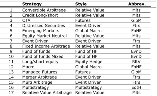
In this regard Table 1 shows the reported strategies found in our dataset, after specific outlier treatment (see section 2.2). These strategies were further grouped by style. Although we believe that the asset allocation discipline creates natural links among some strategies, the classification remains subjective.
In particular, as for the funds of hedge funds, their assets are themselves hedge funds (which can have the same investment style or even different ones), therefore they are not an actual investment style, but we took the liberty to group these funds as a style on its own to simplify the reporting of research output.
Table 1 Reported strategies in dataset
Strategy Style Abbrev.
1 Convertible Arbitrage Relative Value Mlts 2 Credit Long/short Relative Value Mlts
3 CTA Futures GlbM
4 Distressed Securities Event Driven Ftrs
5 Emerging Markets Global Macro FoHF
6 Equity Market Neutral Relative Value Mlts
7 Event Driven Event Driven Ftrs
8 Fixed Income Arbitrage Relative Value Mlts
9 Fund of funds Fund of HF EvnD
10 Fund of funds Mixed Fund of HF EvnD 11 Long/short equity Equity Hedge RltV
12 Macro Global Macro FoHF
13 Managed Futures Futures GlbM
14 Merger Arbitrage Event Driven Ftrs
15 Multi Arbitrage Event Driven Ftrs
16 Multistrategy Multistrategy EqtH
17 Relative Value Arbitrage Relative Value Mlts
Note: Fund strategies are those reported by managers. Style grouping is ours. ‘Funds of funds’ are listed as a style for convenience of analysis reporting.
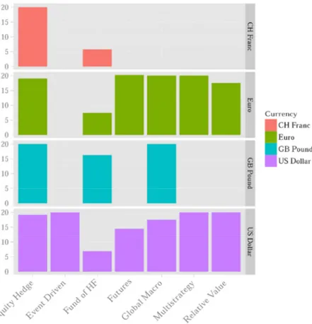
13 Whatever the style (or strategy), the defining hallmark of the hedge funds, as an alternative investment class, is the common active, if not ‘aggressive’, management policies. Both the supplementary costs and the expected benefits of these policies are supposedly charged to the investors in terms of fees. To check out informally these claims, Figure 1, based on the style clusters set in Table 1, shows fee structures distributed by style and currency. Fees are intended as performance fees, calculated as a percentage of the increase in the gross asset value of the fund. Complex fee structures not uniquely representable with a single percentage were not included. All values settle at a high level, except for funds of hedge funds, where, by the way, the investor has to pay twice, since the underlying constituent funds are already subject to their own fees.
Figure 1 Fee structures distributed by style and currency: average performance fee (percentage figures)
Source: Authors' elaboration
We now come to the most relevant piece of data to our research objective, and that is the time series of the funds’ Net Asset Values (henceforth NAV’s). Before indulging in the usual descriptive statistics on risk-return dynamics, we will devote a separate section to the methodology used for outlier detection/removal from the time series. Indeed, the biases mentioned at the beginning of this section and the special nature
of the hedge funds as an asset class motivated us to build a specific filter for outlier management.
2.2 Methodology for Outlier Detection and Management
The biases already described in the previous section might easily yield a fast and possibly not faithful switching return dynamics, which will be observed in the form of outliers in the historical records.
Apart from this, there is a more technical reason beyond the non-smooth dynamic of hedge funds, described by Lo (2005) as “phase-locking” behaviour. This behaviour, well known in the physical and natural sciences, is a situation when two normally uncorrelated patterns suddenly become perfectly synchronized. In financial markets the dramatic switch in correlations can be a consequence of market crises. Hedge funds exhibit nonlinearity and are exposed to phase-locking behaviour, which in turn will involve a sudden jump in returns, observable as outliers.
Finally, the lack of regulations and reporting standards often determines a change of scales in fund NAVs due to changing accounting practices, which is observable in terms of dramatic outliers: e.g. figures reported in millions changing to billions. This effect can be easily checked out by a human reading of the observation records, but is not manageable with ordinary statistical procedures.
We face a trade-off when processing hedge fund databases since on the one hand we face many reporting biases, on the other hand bold speculative policies might result in dramatic variations in fund asset values, which could be falsely clustered as outliers. Common advice for measuring hedge fund performance is to use the median, cf. Chap. 19 in Lhabitant (2011) and Aiken et al. (2012).
Following this, we now describe the procedure used in this study to produce the workable time series.
We selected funds having a continuous track record from January 2005 through to December 2012 (thus the dataset was deeply downsized to obtain comparable time series). Given this criterion, the actual time span used started from January 2006 to deal with backfill bias (so previous observations were discarded, while selected funds were still required to report them). As for survivorship bias, by the scope of this analysis, we are interested in those funds actually available to the investors during the whole time covered by our analysis, that is, how they perform provided that they do (see Dor et al. (2012) for similar arguments).
Given this preliminary dataset, a popular option for outlier treatment is the extreme
studentised deviate more familiarly spelled as the “three-sigma edit rule”, that is, any
point distant more than t standard deviations from the mean of its neighbours is an outlier. Formally, an outlier does not belong to the interval:
[µ^ − tσ^, µ^ + tσ^]
where µ^, σ^ are the sample mean and deviation of the reference neighbourhood. For normal data, it is customary to take 3 as the threshold value t. In fact, for a normal distribution, observing values more than three standard deviations away from
15 the mean is only 0.3% likely, that is, for variable X ∽ N(µ,σ) , P[X > |µ − 3σ|] ≈ 0.99730 Detected outliers are usually replaced with their reference mean (µ^), cf. Pukelsheim (1994).
There is an inherent pitfall with this approach: the mean, and even more the standard deviation, are themselves distorted by outliers. When source data are essentially non-smooth, such as hedge funds, showing skew normal distributions8, this can lead to significant biases in inference.
As an alternative to the “local three-sigma” rule one can use the Median Absolute
Deviation:
MX= m(|X − mX|) (1)
where mX is the median of X.
In this case, (1) uses the median of neighbouring observations as a reference value, and uses the deviation from the median (MAD) as an alternative measure of distance. Given (1), an outlier is such when lying more than t times the MAD from the median of its neighbours. Such a filter is commonly addressed as Hampel filter (see Pearson, 2011).
In this research we used a version of the standard Hampel filter slightly modified as follows:
• After outlier detection, the median was replaced with the average observations before and past the outlier.
• The filter was adjusted at the borders of the series, to avoid cutting data. • The MAD was adjusted by a factor of about 1.5, as it can be shown that for
normal data:
σX≈ 1.4826MX
Eventually we “cleaned” data from missing values or incoherent values (e.g. negative NAVs), by means of interpolations. We also did not include “Asset based lending” and “Mortgage-Backed Securities” funds, since these are beyond the scope of this research.
2.3 Aggregating Funds by Investment Policy
In this section we detail the methodology used to aggregate returns.
Since every fund has a reported strategy (and only one), let the hedge fund (i,j) denote i -th fund among those reporting the j -th strategy. Therefore, rij(th) denotes
the monthly return observed on month h -th (of the time series) for the (i,j) fund. With reference to the time window T = tb− (ta− 1) , the average return for the (i,j)
fund will be:
fij(ta, tb) = Fij(T) = ∑ b h a rij(th) T (2)
8 See Eling et al. (2010).
In the same period the average for j -the strategy will be: sj(ta, tb) = Sj(T) = ∑ nj i 1 Fij(T) nj (3)
where nj is the number of funds comprising j -th strategy.
Given (2) and (3), the average for all funds and strategies during T are resp.:
F(T) = ∑ nj,Ns i,j 1 Fij(T) NF ; S(T) = ∑ Ns j 1 Sj(T) Ns
where NF, NS are resp. the total number of funds, strategies. Obviously NF= ∑ Ns
j 1nj .
The average for all funds during T does not necessarily equal to the average for all strategies, unless the latter are equinumerous, in fact assuming every nj= n:
S(T) = ∑ Ns j 1 ∑n i 1 Fij(T) n Ns = ∑ Ns j 1∑ n i 1 Fij(T) nNs = ∑ Ns j 1∑ n i 1 Fij(T) NF = ∑ Ns j 1Sj(T) (4)
If nj≠ n , the (4) does not hold and to compute the relation between the averages,
depending on how significant the differences are, one should consider redefining S(T) with a weighted average accounting for strategy magnitudes.
As for styles, given the previous strategy-style mapping (see Table 1), the style classification can be thought of as a partition P of the set of all strategies 1 … NS ;
therefore, the k -th style is the set Mk∈ P , where ∀j ∈ Mk j is a strategy mapped to
the k -th style. The average return for this style, with reference to the time window T = tb− (ta− 1) , is: qk(ta, tb) = Qk(T) = ∑ nj i 1 j∈Mk Fij(T) #Mk (5)
where #Mk, the cardinality of Mk, is the number of strategies mapping to the k-th style.
As seen for strategies, by (5), if the style sets (Mk) share the same cardinality, the
average returns for all funds, during T, equal the average among styles.
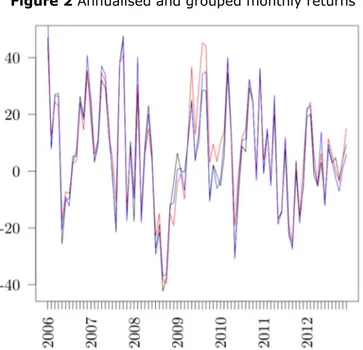
Since the hypothesis of equinumerosity is not consistent with our dataset, for both strategy and style partitions, it makes sense to compare the average returns obtained with and without fund aggregations. Therefore, Figure 2 compares the monthly fund returns contrasting grouped and non-grouped averages. Similarly Table 2 shows the correlation between the series obtained with the different grouping levels. Both the plots and the figures show the differences in the average returns are negligible.
17 Figure 2 Annualised and grouped monthly returns
Note: Black line plots average returns without any grouping. Red line and blue lines plot returns by strategies and styles, respectively.
Source: Authors' elaboration
Table 2 Measuring the Grouping Effect: correlation between different grouping levels
Ungrouped By Strategy By Style
Ungrouped 1.00 0.95 0.98
By Strategy 0.95 1.00 0.96
By Style 0.98 0.96 1.00
Source: Authors' elaboration
2.4 (Reported) Returns: Notes and Descriptive Statistics
To give the reader a preliminary knowledge of returns dynamic, we will show some descriptive statistics related to the return time series obtained by means of the monthly reported NAV, after applying the outlier treatment from section 2.2.
As observed in section 2.3, though average performance for all funds will not necessarily be equal to the average among styles or strategies, return time series proved almost overlapping visually and highly correlated analytically for our dataset. So we can measure the overall return starting from grouped funds with negligible bias.
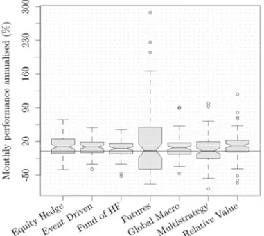
Figure 3 shows distributions of style returns for the time range scrutinised by means of notched boxplots. On average, over the whole period January 2006–December 2012, styles exhibit good performances, with a limited shortfall area. ‘Futures‘ and ‘Multistrategy’ have a null median, but positive returns tend to outweigh negative ones. Indeed, by looking at the boxplot medians, we can say that returns are not normal (as the theory suggests) and skewed toward the positive side.
Figure 3 Distributions of style returns for the time range scrutinised by means of notched boxplots
Note: The overall shape of returns is shown for each style as a notched boxplot. Each notched box extends between the quartiles so that it contains the middle half of the data, as such the
higher it is, the more variable are the style performances. The line in the middle of the box represents the median, and from its position one can assess the distribution symmetry. “Whiskers” extend outside the box for 1.5 times the inter-quartile range, and they let us easily
identify extreme values, which are located outside of the “fences”. Source: Authors' elaboration
2.5 Crisis Window
When investigating the risk-return dynamics, the importance of market crashes for the outcome of the different investment policies is easily agreed upon, but settling the proper crisis window correspondingly is not straightforward. If we want to mold our analysis in a pre and post crisis fashion, it is crucial to have an objective identification of the crisis window, in order to avoid bias due to an ad hoc definition of the crisis.
With reference to the period scrutinised, a number of events can be considered the outbreak of the crisis: most notably the collapse of the investment bank Bear Stearns in March 2008, which triggered a contagion overwhelming several large financial institutions (including Lehman Brothers, Merrill Lynch, Fannie Mae, Freddie Mac, Wachovia, Citigroup).
Anyway, for a formal, non-subjective, definition we resolved to refer to the Business
Cycle Dating Committee of the National Bureau of Economic Research (NBER). The
Committee maintains a business cycle chronology with reference to the U.S. It defines a “recession” as any period occurring between a ‘peak’ and a ‘trough’. According to September 2010 meeting:
19 “A trough in business activity occurred in the U.S. economy in June 2009. The trough marks the end of the recession that began in December 2007 and the beginning of an expansion. The recession lasted 18 months, which makes it the longest of any recession since World War II.” (Business Cycle Dating Committee 2010)
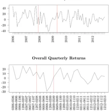
Figure 4 Average monthly and quarterly fund returns (annualised)
Note: Average monthly and quarterly fund returns (annualised) are plotted for comparison with the NBER-identified crisis window. As for monthly returns (left), the pair of red lines mark the crisis beginning month (December 2007) and the crisis ending month (May 2009) according to NBER definitions. As for quarterly returns (right), the quarters are presented on the x-axis with the format ‘mmyy-mmyy’, where each ‘mmyy’ denotes the 2-digit month-year starting and ending the quarter, respectively. The red lines identify the two quarters when crisis started and
ended on NBER terms. Source: Authors' elaboration
Although our analysis is globally scoped, the business cycle reference stems from the US economy. We believe this choice is sounder than the identification of a global, but not as much objective, time window.
Figure 4 helps understanding how (and if) NBER definition applies to hedge funds. As the red plot shows, the worst 18-month period — in term of hedge fund performance — is compatible with NBER definition. The trend of HF monthly and quarterly returns (annualised) is plotted with respect to NBER windows, delimited by the red lines. Their positions are largely consistent with the observed performance of funds, particularly with respect to quarterly returns.
At any rate, since any analysis involving time series is affected by the selected time window, some specific tests will be undertaken to assess the impact of differing time spans, in order to confirm that the crisis period is actually noteworthy.
2.6 Performance Tests9
How different are the simple performances (i.e. without taking risk into account) among different management policies? And particularly how different are under stressed market conditions?
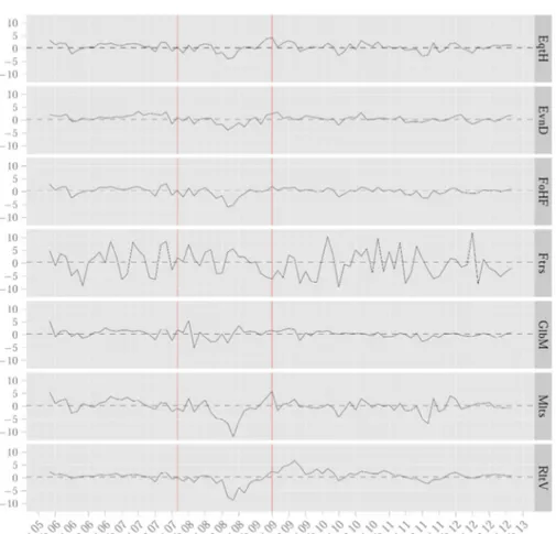
In Figures 5 and 6, we give a preliminary account of the performance dynamics of the industry by styles in histograms and time series format. By applying NBER business cycle findings, we can distinguish the pre-crisis, post-crisis, and crisis periods within the sample. The visual clues we get by these plots show a heterogeneous reaction to cycle switching, and the different nature of performance patterns is possibly amplified during the crisis window, demanding supplementary investigations.
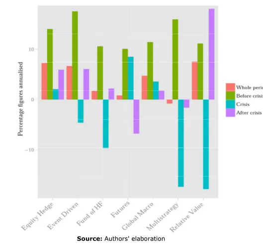
Figure 5 Average style performances with respect to NBER crisis period — December 2007 through to May 2009
Source: Authors' elaboration
9
All statistical tests implemented in this study were carried out via the R language. The main source code is available for interested readers in the Appendix of this paper.
21 One conclusion we might draw is that, as far as the good performance of management styles is a proxy of management skills, talented managers could make the highest difference when the market conditions are tougher; then the crisis can pose profit opportunities for those competent investors capable of timing the market.
Figure 6 Style performance dynamics with respect to NBER crisis period — between the red lines. The dashed line is the overall mean.
Source: Authors' elaboration
To test our hypothesis on return dynamics in a formal way we turn to statistical inference. Using an ANOVA analysis, we check if the differences among groups are significant. We will replicate this analysis with respect to crisis and non-crisis periods, to test if the results hold or possibly amplify.
More formally, we employ an F-test where we assume, as the null-hypothesis, that on average strategies are indistinguishable, this is to say that mean returns are the same. Therefore, given the average return of the i-th strategy µi:
:
=
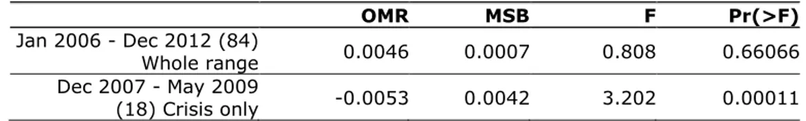
Table 3 shows the result of this test. Here, mean square between (MSB) can be considered a measure of the performance variability among strategies and this variability can be seen as an effect of the diverse management strategies. The usual meaningfulness is assessed by means of p-value, involving rejection of the null hypothesis.
In terms of p-value there is a clear effect of the crisis on the variability of the returns: market stress implies a better capacity to distinguish one management policy (strategy) from another.
Although the test significance is marked, the non-smooth nature of hedge fund returns might expose standard tests to weakness. One path to make the results more robust is to compare the p-value obtained from the target time window, December 2007-May 2009, against the p-values from a random time window.
Preliminarily to this procedure, in Figure 7 we analyse the 18-month overall moving average: a time span which matches the length of NBER crisis window. The upper panel shows the whole dataset period and the lower panel details the windows closer to NBER specification (about 2008-2010). As it follows, the NBER period is not the worst period in terms of hedge fund performance, but there is a slight one month difference.
As anticipated, given high inter-strategy variability observed with respect to the NBER-window, we now test if equally significant results will be obtained for a different time window.
To check this hypothesis, we take all possible 18-month time windows for the dataset period and run the same test for all of them. The battery of tests provides us with a
p-value for each period; therefore, Figure 8 presents, for each 18-month window,
both the average observed return and the p-value assessing the test significance (i.e. the level of return variability among strategies for the given period). To plot the p-values visually, we plot −log10(p) . In this way, a value like ‘2’ can be considered a significant level. Figure 8 partly confirms previous results, but also adds new insights. The p-values follow the trend of the related period and they appear connected to both upward and downward peaks. The policy difference is significant in cycles which show non-average returns, in both cases the management policies can make difference in results.
Table 3 The performance variability among strategies
OMR MSB F Pr(>F)
Jan 2006 - Dec 2012 (84)
Whole range 0.0046 0.0007 0.808 0.66066
Dec 2007 - May 2009
(18) Crisis only -0.0053 0.0042 3.202 0.00011
Note: The performance variability among strategies is measured by means of an F-test. As usual the OMR is the overall mean and MSB the mean squares between groups, with reference
to monthly return. Source: Authors' elaboration
23 Figure 7 18-month moving average returns aggregating all strategy clusters
Note: The upper panel plots the whole sample period. The lower panel gives a detail for the windows next to the NBER crisis window. As for the latter, each point on the x-axis of the lower
panel denotes an 18-month window using the format ‘mmyy-mmyy’, where each ‘mmyy’ denotes the 2-digit month-year beginning and ending the related window, respectively. The
moving average is the rolling geometric mean. Source: Authors' elaboration
Source: Authors' elaboration
2.7 Alternative Approaches to Risk
The comparison among policy returns is financially meaningful only if backed by the risk born by each policy. This suggested creating a measure embedding both the premium and the risk involved in an alternative investment.
To this end, we introduce a measure denoted Alternative Excess Return (AER), trying to assess the premium of the alternative investment over a traditional one while weighting the extra risk carried. In schematic terms:
! =A"TDD = DD#$
Here the numerator represents the flat AER, that is, the excess return of the alternative return (A) over the traditional return (T); the denominator is the “dynamic downside risk” of the premium (DD), i.e. the zero-based semideviation of the AER.
25 is relative to the market condition: in a bear market it is sufficient not to do as bad as the (traditional) market; but in a bull market a downside is obtained when the alternative asset is unable to get returns as high as a traditional portfolio.10
D-AER was tested with historical data, proxying the traditional returns with the S&P500 index.
We start the analysis by plotting (Figure 9) frequency polygons relative to the D-AER distribution, for each style identified. The right half of the distribution identifies the observations where the alternative investments give a premium over the traditional choice.
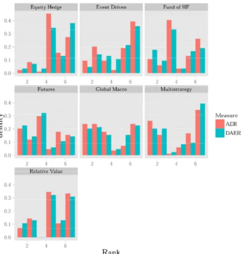
We note that “Relative Value” and “Equity Edge” styles show a similar (partly overlapping) right skewed distribution. The peak area of the “Event Driven” is symmetric, but the tails, which attract the large part of the observations, are right skewed. These styles will require further testing to confirm the visual behaviour. Figure 10 compares D-AER against flat AER premia through “dodged” histograms for each style. Since measures use different scales, for each measure, style performances are ranked in an increasing order, from one to seven, and the bars of the relative performances (performance ranks) are plotted.
In general AER and D-AER patterns tend to “intersect”: for any style, no measure prevails and there are several inversions along the ranking scale.
“Equity Edge”, “Event Driven”, and “Relative Value” styles appear to show the highest frequencies in the upper rankings and the lowest frequencies in the inferior rankings. To confirm the visual clues, we tested the significance of the alternative premium with two statistical tests: a binomial test, where the “success” is defined as obtaining a positive D-AER instead of a negative one; a Student t-test, measuring the intensity of this success. Therefore, the former is influenced only by the sign of the premium and the latter by its dimension too.
10 Note that D-AER, is not functionally or algorithmically equal to the Sortino ratio. The
numerator performance measure (AER) is not based on a fixed target or Minimum Acceptable Return (MAR), but on a period by period comparison with the benchmark; the denominator risk measure is not the downside risk of the alternative portfolio with respect to the MAR, but is the semideviation of the AER taking the zero as the reference point. Given this, when compared with a Sortino ratio using the same benchmark returns over the same period, the downside adjusted AER ratio takes also into account the correlation of the alternative portfolio with the target traditional portfolio and “dynamically” adjusts for variations of the traditional portfolio; cf. Rom and Ferguson 2001, Fasano and Minnetti 2012.
Note: Each polygon is the D-AER distribution of the colour-coded style given in the legend. The more the distribution is right skewed, the more the alternative investment gives a
(risk-weighted) premium over the traditional one. Source: Authors' elaboration
27
Note: For both measures monthly style performances are ranked from 1
(lowest performance) to 7 (highest performance). The histograms show the distribution of ranks for each style over the sample period.
Source: Authors' elaboration
Table 4 shows the results of these tests. The inference outcomes tend to confirm the outcomes from the plotted data. For some styles, during the period under investigation, the alternative premium is positive, even considering the risk factor;
besides, their average is significant.
Specifically, in terms of t-test, i.e. of the “intensity” of the premium, the “Equity Edge” and “Event Driven” styles show a significant better risk adjusted performance compared to a traditional investment.
success Bin. p-value D-AER t p-value Event Driven 0.48 0.707 0.3050 0.013 Equity Hedge 0.46 0.777 0.2626 0.025 Relative Value 0.43 0.922 0.1688 0.092 Global Macro 0.42 0.949 0.1707 0.107 Fund of HF 0.43 0.922 0.0266 0.418 Futures 0.39 0.981 -0.0341 0.593 Multistrategy 0.43 0.922 -0.0693 0.698
Note: The first two columns report a binomial test of AER positivity: they are the realised “success” ratio and its significance, respectively. The following columns measure the intensity of
AER: they are respectively the mean AER and its significance. Source: Authors' elaboration
3 Results
The analysis of fund performances, without taking the risk into account, shows that different management policies can make a significant difference when the market conditions are tougher.
Stressed market conditions emphasize talented managers, to whom crises can pose profit opportunities.
ANOVA analysis, concerning funds grouped by managers’ reported strategies, shows significant inter-group differences during the crisis period. This result is further confirmed by a non-parametric analysis, where randomly generated time windows are compared with the actual crisis window.
As regards risk measures and risk-adjusted performances, we built two specific measures representing the risk premia involved in alternative investments:
• Alternative Excess Return (AER), the excess return of an alternative investment over a traditional investment;
• D-AER, AER scaled with the downside risk.
The risk analysis involved a binomial test and a t-test: the former capturing only the better alternative (from the alternative and traditional investments); the latter giving also the intensity of premia (if any).
A number of HF styles yield better results on average. Also, the means prove statistically significant with respect to Event Driven and Equity Hedge styles.
Conclusions
In this study, we addressed the risk-return dynamic of hedge fund alternative investments, given the presence of distressed market conditions and with reference to the crisis window set by NBER Business Cycle Dating Committee. We also distinguished the analysis by the management policies applied, although there is no formal taxonomy in this regard, under the assumption that they can be intended as a proxy of the management portfolio selection skills. After analysing the management policies of hedge funds, we introduced a new metric for assessing the alternative
29 First, we found that the crisis had the effect of emphasizing the differences among the management policies. Under market pressure, management styles are not all equal: the different approaches turn into different possibility of ruin, safety, or even profit.
We further extended this analysis and found that the significance of management skills is emphasized by market trends. When the market is flat, the manager makes little difference, when the market changes regime (both bear and bull), test significance increases, signalling that skilled fund strategists can turn their ability to anticipate price movements into profits.
To better assess the quality of these policies we developed a measure of the excess return gained going alternative (AER), scaled with the downside risk dynamically targeted to a traditional investment portfolio (D-AER). The alternative investment is rewarding, for some styles, that is, we found that the D-AER is historically positive on average and statistically significant.
References
Ackermann, C., McEnally, R., Ravenscraft, D. (1999). The Performance of Hedge Funds: Risk, Ieturn, and Incentives. The Journal of Finance, 54(3), pp. 833–874. Agarwal, V., Naik, N. Y. (2000). Multi-period Performance Persistence Analysis of Hedge Funds. Journal of Financial and Quantitative Analysis, 35(03), pp. 327–342. DOI 10.2307/2676207.
Agarwal, V., Naik, N. Y. (2004). Risks and Portfolio Decisions Involving Hedge Funds.
Review of Financial Studies, 17(1), pp. 63–98. DOI 10.1093/rfs/hhg044.
Agarwal, V., Fos, V., Jiang, W. (2013). Inferring Reporting-related Biases in Hedge Fund Databases from Hedge Fund Equity Holdings. Management Science, 59(6), pp. 1271–1289. DOI 10.1287/mnsc.1120.1647.
Agarwal, V., Daniel, N. D., Naik, N. Y. (2009). Role of Managerial Incentives and Discretion in Hedge Fund Performance. The Journal of Finance, 64(5), pp. 2221– 2256. DOI 10.1111/j.1540-6261.2009.01499x.
Aiken, A. L., Clifford, C. P., Ellis, J. (2012). Out of the Dark: Hedge Fund Reporting Biases and Commercial Databases. Review of Financial Studies, hhs100. DOI 10.1093/rfs/hhs100.
Amenc, N., Martellini, L. (2003). The Brave New World of Hedge Fund Indices. Tech. rep. Edhec/Misys multi-style/multi-class research program. DOI 10.1.1.123.5975. Ammann, M., Moerth, P. (2005). Impact of Fund Size on Hedge Fund Performance.
Journal of Asset Management, 6(3), pp: 219–238. DOI 10.1057/palgrave.jam.2240177.
Aragon, G. O. (2007). Share Restrictions and Asset Pricing: Evidence from the Hedge Fund Industry. Journal of Financial Economics, 83(1), pp: 33–58. DOI 10.1016/j.jfineco.2005.11.001.
Bacmann, J.-F., Pache, S. (2003). Optimal Hedge Fund Style allocation under higher moments. Tech. rep. Intelligent Hedge Fund Investing.
Bali, T. G., Brown, S. J., Caglayan, M. O. (2011). Do Hedge Funds’ Exposures to Risk Factors Predict their Future Returns? Journal of Financial Economics, 101(1), pp: 36– 68. DOI:10.1016/j.jfineco.2011.02.008.
Baquero, G., Ter Horst, J., Verbeek, M. (2005). Survival, Look-ahead Bias, and Persistence in Hedge Fund Performance. Journal of Financial and Quantitative
Analysis, 40(3), pp: 493–517. DOI 10.1017/S0022109000001848.
Barès, P.-A., Gibson, R., Gyger, S. (2003). Performance in the Hedge Funds Industry: An Analysis of Short-and Long-term Persistence”. The Journal of Alternative
Investments, 6(3), pp: 25–41. DOI 10.3905/jai.2003.319097.
Billio, M., Getmansky, M., Lo, A. W., Pelizzon, L. (2010). Measuring Systemic Risk in the Finance and Insurance Sectors. Tech. rep. Alfred P. Sloan School of Management, Massachusetts Institute of Technology. DOI 1721.1/66679.
Boyson, N. M., Stahel, C. W., Stulz, R. M. (2010). Hedge Fund Contagion and Liquidity Shocks. The Journal of Finance, 65(5), pp: 1789–1816. DOI 10.1111/j.1540-6261.2010.01594x.
Brooks, C., Kat, H. (2002). The Statistical Properties of Hedge Fund Index Returns and their Implications for Investors. Journal of Alternative Investments, 5(2), pp: 26– 44. DOI 10.3905/jai.2002.319053.
Brown, S. J., Goetzmann, W. N. (2001). Hedge Funds with Style. Tech. rep. National Bureau of Economic Research. DOI 10.3386/w8173.
Brown, S. J., Goetzmann, W. N., Ibbotson, R. G. (1999). Offshore Hedge Funds: Survival and Performance 1989-1995. Journal of Business, 72(1), pp: 91–117. DOI 10.2469/dig.v29.n3.538.
Business Cycle Dating Committee (2010). Announcement of June 2009 business cycle
trough/end of last recession. Tech. rep. National Bureau of Economics Research.
Cao, C., Chen, Y., Liang, B., Lo, A. (2011). Can Hedge Funds Time Market Liquidity? Tech. rep. Available from SSRN 1537925. DOI 10.2139/ssrn.1537925.
Derman, E. (2007). A Simple Model for the Expected Premium for Hedge Fund Lockups. Tech. rep. DOI 10.2139/ssrn.952889.
Ding, B., Getmansky, M., Liang, B., Wermers, R. (2009). Share Restrictions and Investor Flows in the Hedge Fund Industry. Tech. rep. Available at SSRN 891732. Dor, A. B., Berkovitz, Y., Xu., J. (2012). A Quantitative Framework for Analyzing the Performance of an Individual Hedge Fund vs. its Peers. Tech. rep. Cross Asset Research, Quantitative Portfolio Strategy. Barclays Research.
Edwards, F. R., Caglayan, M. O. (2001). Hedge Fund and Commodity Fund Investments in Bull and Bear Markets. The Journal of Portfolio Management, 27(4), pp: 97–108. DOI 10.3905/jpm.2001.319816.
31 Eling, M., Schuhmacher, F. (2007). Does the Choice of Performance Measure Influence the Evaluation of Hedge Funds? Journal of Banking & Finance, 31(9), pp: 2632–2647. DOI 10.1016/j.jbankfin.2006.09.015.
Eling, M., Farinelli, S., Rossello, D., Tibiletti, L. (2010). Skewness in Hedge Funds Returns: Classical Skewness Coefficients vs Azzalini’s Skewness Parameter.
International Journal of Managerial Finance, 6(4), pp: 290–304. DOI 10.1108/17439131011074459.
Fasano, A., Minnetti, F. (2012). Hedge Fund Performances: A Comparison Based on Styles and Strategies. European Journal of Economics, Finance and Administrative
Sciences, 53, pp: 59–80.
Fung, W., Hsieh, D. A. (1997a). Empirical Characteristics of Dynamic Trading Strategies: The Case of Hedge Funds. Review of Financial Studies, 10(2), pp: 275– 302. DOI 10.1093/rfs/10.2.275.
Fung, W., Hsieh, D. A. (1997b). Survivorship Bias and Investment Style in the Returns of CTAs. The Journal of Portfolio Management, 24(1): 30–41. DOI 10.3905/jpm.1997.409630.
Fung, W., Hsieh, D. A. (2000). Performance Characteristics of Hedge Funds and Commodity Funds: Natural vs. Spurious Biases. Journal of Financial and Quantitative
Analysis, 35(03), pp: 291–307. DOI 10.2307/2676205.
Fung, W., Hsieh, D. A. (2002). Hedge-fund Benchmarks: Information Content and Biases. Financial Analysts Journal, 58(1), pp: 22–34. DOI 10.2469/faj.v58.n1.2507. Fung, W., Hsieh, D. A. (2004). Hedge Fund Benchmarks: A Risk-based Approach.
Financial Analysts Journal, 60(5), pp: 65–80. DOI 10.2469/faj.v60.n5.2657.
Getmansky, M. (2004). The Life Cycle of Hedge Funds: Fund Flows, Size and Performance. Working paper. DOI 10.2139/ssrn.686163.
Gregoriou, G. N., Pascalau, R. (2012). A Joint Survival Analysis of Hedge Funds and Funds of Funds Using Copulas. Managerial Finance, 38(1), pp: 82–100. DOI 10.1108/03074351211188376.
Harri, A., Brorsen, B. W. (2004). Performance Persistence and the Source of Returns for Hedge Funds. Applied Financial Economics, 14(2), pp: 131–141. DOI 10.1080/0960310042000176407.
Harris, J. (2010). Hedge Fund Trading Volume Rises as Algorithms Become More Popular. Tech. rep. risk.net.
Howell, M. J. (2001). Fund Age and Performance. The Journal of Alternative
Investments, 4(2), pp: 57–60. DOI 10.3905/jai.2001.319011.
Jagannathan, R., Malakhov, A., Novikov, D. (2010). Do Hot Hands Exist among Hedge Fund Managers? An Empirical Evaluation. The Journal of Finance, 65(1), pp: 217–255. DOI 10.1111/j.1540-6261.2009.01528.x.
Keating, C., Shadwick, W. F. (2002). A Universal Performance Measure. Journal of
Performance Measurement, 6(3), pp: 59–84.
Kim, J.-M. (2008). Failure Risk and the Cross-section of Hedge Fund Returns.
Working Paper.
Kosowski, R., Naik, N. Y., Teo, M. (2007). Do Hedge Funds Deliver Alpha? A Bayesian and Bootstrap Analysis. Journal of Financial Economics, 84(1), pp. 229–264. DOI 10.1016/j.jfineco.2005.12.009.
Lamm Jr, R. M. (2003). Asymmetric Returns and Optimal Hedge Fund Portfolios. The
Journal of Alternative Investments, 6(2), pp: 9–21. DOI 10.3905/jai.2003.319088.
Le Moigne, C., Savaria, P. (2006). Relative Importance of Hedge Fund Characteristics. Financial Markets and Portfolio Management, 20(4), pp: 419–441. DOI 10.1007/s.11408-006-0029-z.
Lhabitant, F.-S. (2011). Handbook of hedge funds. John Wiley & Sons.
Liang, B. (1999). On the Performance of Hedge Funds. Financial Analysts Journal, 55(4), pp: 72–85. DOI 10.2469/faj.v55.n4.2287.
Liang, B. (2000). Hedge Funds: The Living and the Dead. Journal of Financial and
Quantitative Analysis, 35(3), pp: 309–326. DOI 10.2307/2676206.
Liang, B., Park, H. (2007). Risk Measures for Hedge Funds: A Cross-sectional Approach. European Financial Management, 13(2), pp: 333–370. DOI 10.1111/j.1468-036X.2006.00357.x.
Lo, A. W. (2005). The Dynamics of the Hedge Fund Industry. Research Foundation of CFA Institute.
Malkiel, B. G., Saha, A. (2005). Hedge Funds: Risk and Return. Financial Analysts
Journal, 61(6), pp: 80–88. DOI 10.2469/faj.v61.n6.2775.
Mancini, L., Ranaldo, A., Wrampelmeyer, J. (2011). Internet Appendix for Liquidity in the Foreign Exchange Market: Measurement, Commonality, and Risk Premiums. Tech. rep. DOI 10.2139/ssrn.1974419.
Martin, G. (2001). Making Sense of Hedge Fund Returns: A New Approach. Chap. 9 in
Added Value in Financial Institutions: Risk or Return?, ed. by E. Accar, pp: 165–182.
Prentice-Hall, Upper Saddle River, New Jersey.
Mitchell, M., Pulvino, T. (2001). Characteristics of Risk and Return in Risk Arbitrage.
The Journal of Finance, 56(6), pp: 2135–2175.
Pearson, R. K. (2011). Exploring Data in Engineering, the Sciences, and Medicine. Oxford University Press.
Perelló, J. (2007). Downside Risk Analysis Applied to the Hedge Funds Universe.
Physica A: Statistical Mechanics and its Applications, 383(2), pp: 480–496. DOI
10.1016/j.physa.2007.04.079.
Pukelsheim, F. (1994). The Three Sigma Rule. The American Statistician, 48(2), pp: 88–91. DOI 10.1080/00031305.1994.10476030.
33 in Managing Downside Risk in Financial Markets, ed. by F. A. Sortino and S. Satchell, pp. 59–73. Butterworth-Heinemann.
Sadka, R. (2010). Liquidity Risk and the Cross-section of Hedge-fund Returns.
Journal of Financial Economics, 98(1), pp: 54–71. DOI 10.1016/j.jfineco.2010.05.001.
Schneeweis, T., Spurgin, R. B. (1998). Multifactor Analysis of Hedge Fund, Managed Futures, and Mutual Fund Return and Risk Characteristics. The Journal of Alternative
Investments, 1(2), pp: 1–24. DOI 10.3905/jai.1998.407852.
Schneeweis, T., Spurgin, R. B., McCarthy, D. (1996). Survivor Bias in Commodity Trading Advisor Performance. Journal of Futures Markets, 16(7), pp: 757–772. DOI 10.1002/(SICI)1096-9934(199610)16:7<757::AID-FUT2>3.0.CO;2-N.
Schneeweis, T., Kazemi, H. B., Martin, G. A. (2002). Understanding Hedge Fund Performance: Research Issues Revisited-part I. The Journal of Alternative
Investments, 5(3): 6–22. DOI 10.3905/jai.2002.319061-
Sharpe, W. F. (1992). Asset Allocation Management Style and performance measurement. The Journal of Portfolio Management, 18.2, pp: 7–19. DOI 10.3905/jpm.1992.409394.
Shawky, H. A., Dai, N., Cumming, D. (2012). Diversification in the Hedge Fund Industry. Journal of Corporate Finance, 18(1), pp: 166–178. DOI 10.1016/j.jcorpfin.2011.11.006.
Sortino, F. A., Price, L. N. (1994). Performance Measurement in a Downside Risk Framework. The Journal of Investing, 3(3), pp: 59–64. DOI 10.3905/joi.3.3.59. Sortino, F. A., van der Meer, R., Plantinga, A. (1999). The Dutch Triangle. The