Computing fast search heuristics for physics-based mobile robot motion planning

(1)

based Mobile Robot Motion Planning

Ph.D. in Engineering in Computer Science

Dottorato di Ricerca in Ingegneria Informatica – XXIX Ciclo

Candidate Federico Ferri ID number 1151532

Thesis Advisor Prof. Fiora Pirri

A thesis submitted in partial fulfillment of the requirements

for the degree of Doctor of Philosophy in Engineering in Computer Science September 2018

(2)

Thesis defended on 7 September 2017

in front of a Board of Examiners composed by: Prof. Paolo Boldi (chairman)

Prof. Fabio Massimo Zanzotto Prof. Filippo Furfaro

Computing Fast Search Heuristics for Physics-based Mobile Robot Motion Plan-ning

Ph.D. thesis. Sapienza – University of Rome

This thesis has been typeset by LA_{TEX and the Sapthesis class.}

Version: September 3, 2018

(3)

(4)

iii

Abstract

Mobile robots are increasingly being employed to assist responders in search and rescue missions. Robots have to navigate in dangerous areas such as collapsed buildings and hazardous sites, which can be inaccessible to humans. Tele-operating the robots can be stressing for the human operators, which are also overloaded with mission tasks and coordination overhead, so it is important to provide the robot with some degree of autonomy, to lighten up the task for the human operator and also to ensure robot safety.

Moving robots around requires reasoning, including interpretation of the environment, spatial reasoning, planning of actions (motion), and execution. This is particularly challenging when the environment is unstructured, and the terrain is harsh, i.e. not flat and cluttered with obstacles. Approaches reducing the problem to a 2D path planning problem fall short, and many of those who reason about the problem in 3D don’t do it in a complete and exhaustive manner.

The approach proposed in this thesis is to use rigid body simulation to obtain a more truthful model of the reality, i.e. of the interaction between the robot and the environment. Such a simulation obeys the laws of physics, takes into account the geometry of the environment, the geometry of the robot, and any dynamic constraints that may be in place.

The physics-based motion planning approach by itself is also highly intractable due to the computational load required to perform state propagation combined with the exponential blowup of planning; additionally, there are more technical limitations that disallow us to use things such as state sampling or state steering, which are known to be effective in solving the problem in simpler domains.

The proposed solution to this problem is to compute heuristics that can bias the search towards the goal, so as to quickly converge towards the solution.

With such a model, the search space is a rich space, which can only contain states which are physically reachable by the robot, and also tells us enough information about the safety of the robot itself.

The overall result is that by using this framework the robot engineer has a simpler job of encoding the domain knowledge which now consists only of providing the robot geometric model plus any constraints.

(5)

List of Figures

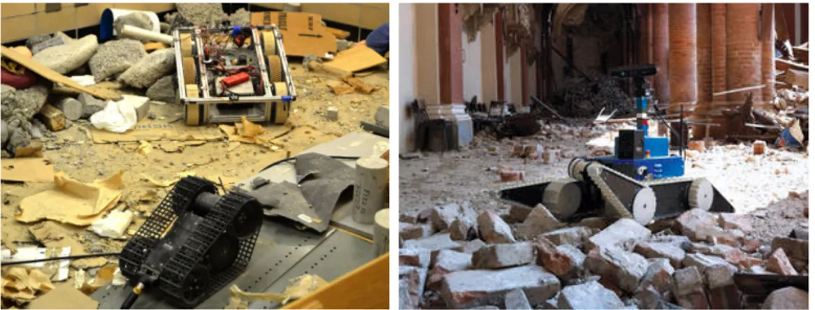
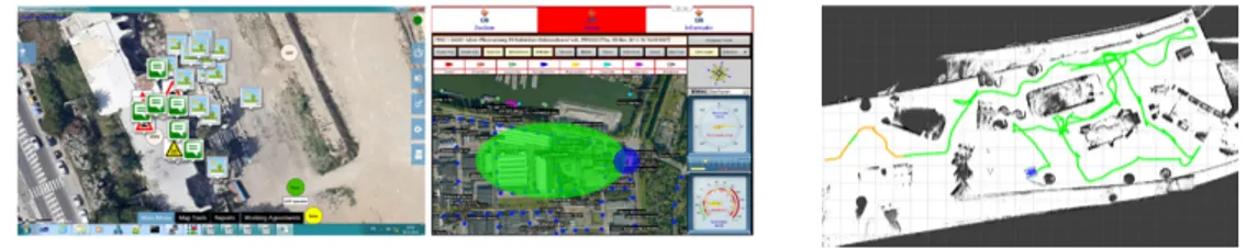
1.1 Mobile robots navigating through rubble in disaster areas. On the left: multiple search and rescue robots moving in a simulated disaster environment. On the right: mobile robot from TRADR project navigating amongst the remains of a collapsed church. . . 1 1.2 Actual search and rescue environments scenarios. . . 2 1.3 Human operators interface used to coordinate mission in TRADR EU

project. . . 2 1.4 Classical occupancy maps in robotics: left: Centibots [Vin+08]; center:

Grand Challenge [Mon+06]; right: Learning Applied to Ground Robots [Kon+08]. . . 3 1.5 3D map of an outdoor environment in the form of a point cloud,

acquired by a robot during navigation using a tilting LIDAR sensor. in the few initial movements the robot is able to gather a significant amount of points describing its surroundings, in a range large enough to allow motion planning on it. . . 5 1.6 A geometrical representation of the "Dubins Car", a very simple model

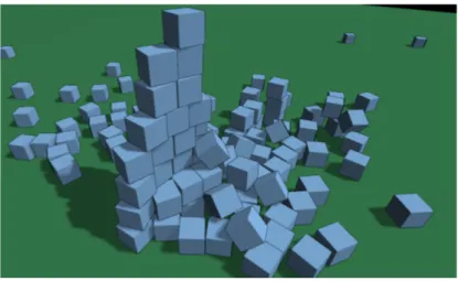
of a four wheeled steering car that can move along Dubins curves [Dub57], and one of the first kinematic models used in motion planning for mobile robots. . . 7 1.7 A screen snapshot of a realtime physics simulator performing a

simula-tion of many cuboidal bodies. The simulator has to take into account gravity force, and thousands of interaction forces caused by each body colliding with several other bodies . . . 9 1.8 Example of a navigation function. Left: a planar map, with start and

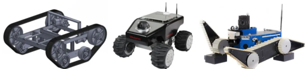
goal locations marked respectively in red and blue; right: navigation function, color-mapped, computed for the goal location. Note that the function is defined only for locations which are connected to the goal location. . . 10 1.9 Some types of mobile robots used for search and rescue, planetary

exploration, and other similar tasks. . . 11 1.10 Left: a cylinder geometry. Right: a capsule geometry. . . 11

(9)

1.11 Modelling a track via a chain of rigid geometries (left) versus a single rigid geometry and contact joints (right). . . 12 3.1 On the left: a triangle-shaped robot that can only translate in a

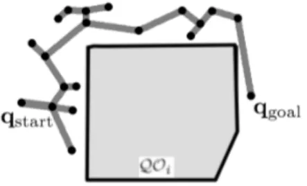
2D workspace. The robot’s reference point is its point. Center: the workspace with one obstacle (WO_i). On the right: the obstacle mapped to the configuration space. The configuration space has size 2 because the two degrees of freedom of the robot. In the configuration space the robot is mapped to a point: if the ploint lies in the free space, then the robot is not in collision with the workspace, and vice-versa. . . 19 3.2 Solution to a motion planning problem found with a sampling-based

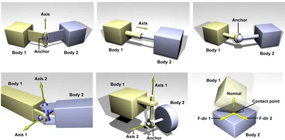
planner. The path connecting qstart to qgoal is entirely in Cfree. . . . 20 4.1 Some examples of joints. From left to right, top to bottom: a hinge

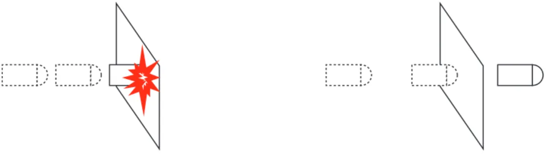
joint (also known as revolute joint); a piston join (also known as prismatic joint); a ball and socket joint (also known as spherical joint); a universal joint; a double hinge joint; a contact joint. Image courtesy of [Smia]. . . 27 4.2 An example of what happens when the collisions are only checked

at discrete steps and not continuously: a bullet moving at a velocity significantly higher than the framerate, such that the displacement of the object between two frames is larger than the object size, will pass through a thin geometry without registering collision. . . 30 5.1 A mobile robot model, with some designated contact zones shown in

red. Collisions happening within the red regions are considered valid. Any other collisions will cause the state to be considered invalid. . . 33 5.2 The RRT algorithm consists of repeating these five operations: 1) pick

a random sample in the search space 2) find the nearest neighbor of that sample 3) select an action from the neighbor that heads towards the random sample 4) create a new sample based on the outcome of the action applied to the neighbor 5) add the new sample to the tree, and connect it to the neighbor. . . 36 5.3 The RRT algorithm. . . 37 5.4 A diagram illustrating the architecture of the physics-based motion

planner: the tree of trajectories is built iteratively and incrementally (e.g.: upon receiving a new query); if the goal has not been reached yet, a state is selected from the tree of trajectories for expansion, and several control inputs are sampled, propagated via the physics based simulation, and ranked according to the heuristic function, and the resulting trajectory increment is put back into the tree of trajectories. 39

(10)

List of Figures ix

6.1 Left: a robot with flexible (rubber) tracks. Right: another robot with rigid, chain-like, tracks. . . 41 6.2 Section of steel track with center sprocket holes to avoid track slipping

off. . . 42 6.3 The tracks modeled as a chain of identical geometries. Each element

is connected to the next element via a hinge joint. In addition, the elements are connected to the planar joint, to avoid slipping away while driving on curved paths. . . 43 7.1 The solution found by the physics-based motion planning described

in chapter 5: due to lack of state-steering, the path (green) cannot be optimized. Also, lots of motions (light gray) are expanded which are not relevant to the solution. . . 46 7.2 Algorithm for heurstics. Above: initialization of data structures (to

be run each time map or goal changes). Below: pointwise function H computing heuristic distance to goal. . . 48 7.3 Left: point cloud segmentation and labeling. Right: weighted graph

representation of a fire escape stairs scenario.. . . 53 7.4 Robot overlayed with path on the weighted graph. . . 55 7.5 Above: segmentation of the fire escape stairs, with path drawn in

magenta, and detail of the robot climbing the stairs (from Fire Escape stairs experiment). Below: a composed path of the robot from the gallery up to the top of the ramp and the bridge (from the Full 3D experiment). It is interesting to note that the robot passes under the gallery still following its path, up to the goal . . . 56 7.6 Traversability map T Map computed real-time while the robot is traversing

a home-made rubble pallet, in the lab. The colors indicate the traversabilty cost, from minimal cost (dark blue) to maximal cost (dark red). . . 59 7.7 On the left a plot of the term wCLas a function of the vertex position. The

dashed region represents an obstacle, and the continuous blue line is the cost. On the right the boundary of a point neighborhood, with highlighted the two sets Q1and Q2. . . 60

8.1 The Italian Fire Fighters rescue training area in Prato (IT) . . . 64 8.2 Fire Escape stairs . . . 64 8.3 On the left segmentation of the third experiment map. On the right

a screen shot of the generated graph. . . 65 8.4 Time of computation for both the segmentation and the path planning

(11)

A.1 The above sequence shows the typical problem encountered in 3D maps when not correctly updated; (a) 3D model of a simple scenario with a moving person; (b) point cloud Stof the scene, at time t; (c) new point cloud St+1,

at time t + 1, showing the trail of points of the moving person; (d) top view of the scene subtended by ∆θ and ∆φ which should be empty if the map is correctly updated. . . 69 A.2 Basic LIDAR system mounted on a servomotor. . . 71 A.3 Spherical wedge V_i,j,k delimited by the intervals P_i, Θ_j and Φ_k in

spherical coordinates on the left and in cartesian coordinates on the right. . . 72 A.4 (left) detecting the points to remove in presence of background and

(right) failing to detect points to remove due to lack of background. . 74 A.5 Set of spherical wedges and w_i,j,k of Scan_t+1 and S_t for fixed j and k.

Highlighted in Scan_t+1the occupied wedge, and highlighted in S_tthe wedge and the points, which will not be merged into S_t+1. Observe that in Scant+1 some outliers appear, which could have affected the

(12)

1

Chapter 1

Introduction

Mobile robot navigation in harsh terrain is a challenging task. Although tracked robots are well equipped to operate in clutter, they still require a human operator to remotely teleoperate them in search and rescue operations. Improving autonomy for these robots is a pivotal issue in the search and rescue field.

In order to move autonomously and safely in the environment, a mobile robot must understand the effects its own dynamics and of its interactions with the terrain.

Figure 1.1. Mobile robots navigating through rubble in disaster areas. On the left: multiple search and rescue robots moving in a simulated disaster environment. On the right: mobile robot from TRADR project navigating amongst the remains of a collapsed church.

For example in a search-and-rescue setting, a mobile robot must go through rubble and collapsed buildings to locate survivors (see Figure 1.1).

Motion planning is the key aspect of robot locomotion which, given a map, a robot geometry, a start position and a goal position, aims to find a path for the robot which is free from collisions.

(13)

1.1 Motivation

The role of Robots in Search and Rescue environments Mobile robots

are increasingly being employed to assist responders in search and rescue missions. Robots have to navigate in dangerous areas such as collapsed buildings and hazardous sites, which can be inaccessible to humans (see Figure 1.2). In the last decades, rescue robots participated in many of the most critical environmental disasters around the world, exhibiting extraordinary abilities in terms of mapping, vision and navigation. In northern Italy, where the city Mirandola was hit by a tremendous earthquake in June 2012, we deployed a team of humans and robot to assess damage to historical buildings and cultural artefacts located therein. This in-field experience has been really important because it led us to a better understanding of what are the main research challenges which are not yet widely addressed in rescue robotics.

Figure 1.2. Actual search and rescue environments scenarios.

During these missions we were able to observe how the human search and rescue operators interacted with the robots and the robot’s software (see Figure 1.3), and we got an understanding of how the software platform can and should be improved.

Figure 1.3. Human operators interface used to coordinate mission in TRADR EU project.

One critical issue the operators encountered concerned the robot’s mobility and locomotion: the task of driving the robot around via remote controls, using only cameras and 3D LIDAR sensors proved to be very demanding for the human operators, and highly error prone. It could happen that subtle variations on the terrain surface can go unnoticed when looked at through a camera or a point cloud, can turn out to be a critical obstacle that can easily make the mobile robot stuck, and require complex maneuvers to get out of that. Motions can sometimes be fatally dangerous to the robot, for example the robot can tip over or fall into a hole. So

(14)

1.1 Motivation 3

this task is supervised by several human operators, looking at various robot sensory data, in order to ensure maximum safety when driving the robot around.

To overcome the amount of cognitive load required to operate the robot, the operator could benefit from any computational aid that could be applied in this domain, from autonomous terrain adaptation (for articulated robots) to autonomous driving (motion planning) in known map areas, or autonomous exploration in unknown areas. Many of these approaches are already being used successfully in several search and rescue exercises. However path planning and autonomous driving is the most challenging task, and the one that could bring the greatest benefit to the search and rescue task.

Typical state-of-the-art methods use a planar representation of the environment (occupancy maps). These maps provide a binary classification of the environment into obstacle/free regions, that overly simplifies the interaction between the mobile robot and the world (see Figure 1.4).

For one reason, the classification of a region into obstacle can be dependent on context, for example a ledge that acts as an obstacle when approached from a lower level, but acts as the ground while the robot is on it. To solve this, sometimes digital elevation maps [Kwe+92] (also known as cartesian elevation maps [Dai+88; Oli+91]) are used instead of binary occupancy 2D maps.

Figure 1.4. Classical occupancy maps in robotics: left: Centibots [Vin+08]; center: Grand Challenge [Mon+06]; right: Learning Applied to Ground Robots [Kon+08].

Moreover, neither 2D maps or elevation maps are able to represent environments with multiple overlapping levels, such as tunnels or multi-storey buildings, but are limited to the representative power of a Monge patch (z = f (x, y)).

Due to the typical terrain conditions usually encountered in this domain, maximum safety has to be guaranteed in order to ensure that a robot motion is really without any risk of losing or damaging the robot, so a 3D representation should be preferred.

(15)

1.2 Problem Statement

The general problem this thesis aims to solve is finding collision-free paths for mobile robots moving in a 3D environment, from a starting position to a goal position, with emphasis to navigation in challenging terrain.

The concept of challenging terrain can be summarized in all those types of terrains for which is not possible to reduce the motion planning problem to a simpler problem, i.e. 2D planning. Challenging terrains are typical of rescue environments and present a quantity of discontinuities and other problems so as to prevent the use of state of the art techniques to map the 3D surface to a manifold and assume that it is entirely traversable.

1.2.1 Assumptions

In order to solve the problem, some fundamental assumptions must hold, namely the availability of the 3D models of the robot and the environment.

Moreover, the environment is assumed to be static for the duration of the planning, and its model is updated only before or after a new motion planning query.

How to obtain these models, as well as how to estimate or model dynamic environ-ments is out of the scope of this thesis.

Model of the robot The 3D model of the robot is known beforehand; it specifies the locomotion devices used such as tracks, legs, wheels, and any other joints and links the robot has to use while moving. Additional information such as mass and inertia is also required, for reasons that will be clarified in the next sections. All these specifications describe the robot in a sufficient way to allow planning the motion of the robot in advance.

Map of the environment A map of the environment in the form of a 3D model is also required.

While a 3D model of the environment is usually not available in domains such as search and rescue, it can be obtained from 3D reconstruction of point clouds (see Figure 1.5) obtained with robot mapping.

In real life scenario, an UAV is first sent to make a first assessment of the area, and that gives us a first 3D model (or point cloud) of the environment.

In lack of that, the initial map seen by the robot’s laser scanner in the starting position is enough to allow the robot to move around to some extent. Typical laser

(16)

1.2 Problem Statement 5

range finders have a range of 10 meters.

Vision based sensors can sometimes be unable to see all the terrain due to occlusion. Although motion planning can only plan the motion of the robot within the known parts of the environment, as the robot moves around, more map of the environment is acquired. The process of moving the robot (via motion planning) to strategic points in the known map, in order to acquire the missing parts of the map, is known as next best view selection, and it is not discussed in this thesis. More can be found in [Yam97; Gon+02; Sur+03; Wen+06; Str+08; Blo+11; Pot+13; Dor+13; Nik]. Instead it will be assumed that the part of the map relevant to the motion planning problem it is already available.

Figure 1.5. 3D map of an outdoor environment in the form of a point cloud, acquired by a robot during navigation using a tilting LIDAR sensor. in the few initial movements the robot is able to gather a significant amount of points describing its surroundings, in a range large enough to allow motion planning on it.

Static environment The environment shall be assumed to be static. Planning in dynamic environments requires the identification of dynamic obstacles, and estimation of their velocity and paths, and it has not been considered in this thesis.

The considered environments are mostly static, so this assumption makes sense in this context.

To ensure maximum safety, the robot should re-sense the environment as it goes, update the map accordingly, and possibly replan if the map has changed. For this purpose, a method for maintaining a map of a dynamic environment is presented in Appendix A.

(17)

1.3 Challenges in Motion Planning for Mobile Robots

in Harsh Terrain

Providing a reliable mathematical model of the interaction between the robot and the terrain is an extremely difficult task. Finding a path for the robot motion which satisfies all the required geometric and dynamic constraints (which include heading, linear and angular velocities and curvatures) requires solving a system of nonlinear differential equations.

A good kinematic model should accurately predict, basing on the neighboring terrain morphology, if the robot will be capable of driving there and where it will arrive if applying certain control inputs.

Conversely, a bad model will not find all trajectories the real robot is capable of driving over, or worse, if can find a trajectory which is unfeasible to the robot, and it will cause some damage, or getting the robot stuck in some obstacle.

Doing motion planning in such complex environments goes beyond traditional motion planning: the terrain is not flat and the interaction between the robot wheels or tracks with the terrain is difficult to model analytically. While it has been shown that is possible to approximate the terrain with simpler geometries [ORo+79; Che99] or monge patches [Gra97; Vas+10], the resulting equations of motion of the robot are usually very complicated and specific to a robot model.

Moreover the robot can be underactuated or have a variety of kinematic and dynamic constraints that put even more restrictions on the computation of a solution; for example the most obvious constraint is being subject to gravity force, which in turn requires the robot to be in a static equilibrium pose, with at least three points of stable contact with the ground.

In the early years of motion planning [Cho05; LaV06], the dynamics aspect of the problem was not taken into account. Instead, only the geometric aspect of the problem, that is, the robot and the obstacles has been considered, such as the piano movers problem [Sch+83a; Sch+83b; Sch+83c]. Those early approaches focused on the explicit construction of the configuration space, which led to proving that complete algorithms are PSPACE-complete and exponential in time [Rei79; Sch+83a; Bro+85; Sch+88; Can88; Pla+10].

When considering also the dynamics of the problem, we usually talk about kinody-namic planning, whose goal is to synthesize robot motion subject to simultaneous kinematic constraints (such as obstacle avoidance, joint limits), and dynamics con-straints (such as bounds on the velocity, acceleration and force/torque).

Much of the recent progress in motion planning is attributed to the development of sampling-based motion planning algorithms [LaV06; Şuc+08; Şuc+09]. Those

(18)

1.3 Challenges in Motion Planning for Mobile Robots in Harsh Terrain 7

Figure 1.6. A geometrical representation of the "Dubins Car", a very simple model of a four wheeled steering car that can move along Dubins curves [Dub57], and one of the first kinematic models used in motion planning for mobile robots.

algorithms have weaker guarantees (they are probabilistically complete, which means that if a solution exists, it will be eventually found; on the contrary, if a solution does not exist, this cannot be reported). The first algorithms of this kind were the Probabilistic Roadmap Method (PRM) [Kav+96], Rapidly-exploring Random Trees (RRT) [LaV98] and Expansive Space Trees (EST) [Phi+04]. These planners build a tree of motions in the state space of the robot and attempt to reach the goal state.

These algorithms are better suited for planning the motion of robot arms or free flying bodies; however applying the same methodology to mobile robots poses additional challenges. For example, sampling-based motion planning cannot be applied to a underactuated robot, such as a mobile robot, with the same ease it can be applied to a robot arm. In the case of a robot arm, state sampling and validation simply accounts to selecting a state from its state space which is not in collision with the environment. This does not work with mobile robots, which have to touch the ground in a stable pose, but not collide with the environment in other ways. Sampling a state in this setting is very expensive. Consider building the configuration space C as usual via collision checking of the robot with the environment. The free subset of the configuration space Cfree is not enough to describe a valid pose: a pose where the robot is free-flying in mid air is not in collision, hence it belongs to C_free, yet it is not valid, because it is not touching the ground in a stable pose. We must take into account the effect of gravity as well. Building the subset of C_free of valid poses is expensive because it requires running physics simulation (or an approximation of it) in addition to performing collision checking. Worse, this type of sampling, cannot be done lazily and/or sparsely, because the fact that two poses are

(19)

valid does not mean that we can blindly interpolate between the two and find a safe (collision-free, stable) motion. Under these considerations, seems more practical to run a physics (rigid body) simulation to drive the robot around and observe which states can be reached by operating on the space of the control inputs. The logic of driving the robot around, that is, searching for a path to the goal state, is the same as in traditional sampling based motion planning algorithms (such as RRT), but state sampling has been replaced with control input sampling. Physics simulation is used to expand the search tree, by applying the sampled control input from a state to obtain a resulting state, together with the resulting motion. This step is known as state propagation.

This approach has the advantage that does not require to model any equation of motion or any equation or approximation of the terrain but instead requires only to give a geometric and physical description of the robot (i.e. the 3D model, the joints, the mass and the inertia of each link, the motor torques) and of the environment (terrain, obstacles), letting the physics simulation engine to compute the interaction between the robot and the environment. However, also some limitations exist, such as: the impossibility of doing backwards simulation; the high computational cost of sampling in the state space; the lack of a method for connecting states in the state space (also known as state steering). These limitations make the use of sampling-based much less effective. Some new motion planners exist that are designed specifically for handling the above mentioned limitations in system with complex dynamics, such as Kinodynamic Planning by Interior-Exterior Cell Exploration (KPIECE) [Şuc+08]. However, since sampling based algorithms spend most of their time extending the tree, and this step is done using physics simulation, which is much computationally intensive than integrating equations of motion, this approach lacks the computational efficiency for real-time planning.

(20)

1.4 Challenges in using a Rigid-Body Simulation as State Propagation 9

1.4 Challenges in using a Rigid-Body Simulation as State

Propagation

Physics simulation allows us to simulate complex real physics systems and thus to predict the behavior of a dynamic system. There are two classes of physics simulation, or physics engines: real-time engines and high-precision engines. High-precision engines are more demanding in terms of CPU time, while real-time physics engines allow to compute simulations in real-time, sacrificing some accuracy.

Figure 1.7. A screen snapshot of a realtime physics simulator performing a simulation of many cuboidal bodies. The simulator has to take into account gravity force, and thousands of interaction forces caused by each body colliding with several other bodies

The physics simulation approach is useful when we want to describe the motion of complex systems, which would be too complicate to describe with equations of motions. One example of this is the motion of a mobile robot in uneven terrains: the interaction between the robot’s wheels or tracks and the shape of the terrain is in general too difficult to model analytically while maintaining a good level of approximation of the real terrain morphology.

This plays a central role in a motion planner because it is the part which expands the tree of states and it has to produce motions which match reality. This step is also known as state propagation. Using a physics simulation to compute the state propagation of the robot has its own appeal: it is a declarative approach, i.e. it states what needs to be solved rather than saying how to solve it. Instead of figuring out the equations of motion for a particular robot in a certain approximation model of the terrain, we simply plug into the system the geometric/kinematic description of the robot (3D CAD model, information about joints, actuators, masses and inertia).

However the accuracy of the simulation depends on many factors. A physics simulation is subject to small errors as well, in part due to limits in numerical

(21)

precision, and in part due to the fact that in order to design an efficient simulation, we want to describe the robot with primitive shapes, such as boxes, spheres, cylinders and capsules. Anyway none of these errors pose a problem, since the relevant elements of a robot are already primitive shapes (such as cylinders for wheels).

During a physics rigid body simulation, there are two stages that are run continuously: 1) integrating Newton’s equations of motion 2) checking collisions between bodies and computing resulting forces. These stages are governed by some internals parameters of the simulator (which will be covered in the next chapters). The setting of these parameters can have impact on the accuracy and the degree of realism of the simulation: an incorrect setting of these parameters can even lead to unstable simulations, which are completely useless to our purposes. It is important that the same control input produces a similar effect both in simulation and in reality. To achieve this we perform a calibration so to tune these parameters.

Choosing the physics world as the model, we encounter unavoidable limitations, such as the impossibility of doing backwards simulation, or the inherent property of the system of not being holonomic nor steerable. Many planners rely on state steering functions, or local planners, to connect pairs of configurations. This step would be too computationally inefficient to compute when the underlying model is the physics world, and with a complexity similar to the global planning problem itself.

The other inevitable problem of using a simulation as state propagation, is that is computationally intensive. We might be able to run it faster than realtime, but not with great speedups. And a motion planning algorithm spends most of its CPU time in expanding the tree, so this becomes the bottleneck of the system: we want to waste the least possible time in performing simulation.

In the next section we will se how to avoid wasting CPU cycles expanding regions of the search space which are not useful in finding a valid motion from start to goal, by exploiting empirical knowledge about mobile robot locomotion, in particular by using a navigation function (see Figure 1.8) to prioritize most promising motions.

Figure 1.8. Example of a navigation function. Left: a planar map, with start and goal locations marked respectively in red and blue; right: navigation function, color-mapped, computed for the goal location. Note that the function is defined only for locations which are connected to the goal location.

(22)

1.5 Challenges in Physics Modeling of Mobile Robots 11

1.5 Challenges in Physics Modeling of Mobile Robots

Figure 1.9. Some types of mobile robots used for search and rescue, planetary exploration, and other similar tasks.

Mobile robots have various type of traction and locomotion devices (see Figure 1.9), depending on the performance requirements and terramechanics (wheel—soil in-teraction mechanics). As an extension of the conventional terramechanics theory for vehicles, the terramechanics theory for mobile robots, which is becoming a new research hotspot, is unique and puts forward many new challenging problems. Currently, the most common robot traction types are wheels and tracks with grousers.

Figure 1.10. Left: a cylinder geometry. Right: a capsule geometry.

In case of a wheeled robot, no particular geometric design considerations are re-quired: wheels can be simulated by using cylinder or capsule geometrical shapes (see Figure 1.10). However, it is very important to provide realistic parameters about friction.

On the other hand, there is no standard method of simulating those.

It is possible to create many finite elements, as shown in Figure 1.11, one for each grouser, connected with hinge joints (see chapter 4 and Figure 4.1), and leave

(23)

to the simulation engine the job of computing collisions and response forces (see subsection 4.3.3). Moreover, as it is the case with reality, some method for keeping the track centered must be used. This approach can give a very realistic result, but at the same time has a big computational cost.

Figure 1.11. Modelling a track via a chain of rigid geometries (left) versus a single rigid geometry and contact joints (right).

In order to simulate traction in a cheaper way, another method is to just compute the contact points between the grouser geometry and the terrain mesh (Figure 1.11), and apply a force to those points. This method is an approximation, and does not take into account deformation of the track, neither the slippage of track versus the terrain.

(24)

1.6 Contribution and thesis structure 13

1.6 Contribution and thesis structure

This thesis studies motion planning for mobile robots in harsh terrain and complex environments. The key aspect taken into consideration in this thesis is to use 3D models for the environment and for the robot, instead of projecting everything on a plane. To make an accurate analysis of navigation in such 3D terrains, a motion planning framework using physics simulation as state propagation is used. The principal contribution is a novel heuristic path-planning strategy that can be used as heuristic function for a physics based motion planner. The result obtained is better planning time compared to existing physics based motion planning approaches. The structure the thesis is the following: a comprehensive literature survey of motion planning and related fields is given in chapter 2; then the preliminaries about motion planning are discussed in chapter 3, and the preliminaries about physics simulation, among with issues that may arise when designing a physics simulation for a mobile robot, are discussed in chapter 4; the physics-based motion planning framework is described in chapter 5; the computation of heuristic functions for the physics-based motion planning framework is described in chapter 7; conclusions are given in chapter 8. A method for updating the map in dynamic environments is presented in Appendix A.

(25)

Chapter 2

Literature Review

When the problem of mobile robot motion planning is studied from a theoretical point of view, certain simplifying assumptions are made; the most important simplification made is to assume a two-dimensional workspace. This is very convenient, as the typical mobile robot still has only three degrees of freedom (one rotational and two for translation) to move over the terrain, so this choice allows to compress the representation of robot motion into curves on a plane. This simplification is also very effective in certain environments, such as indoor, planar or structured environments, and to some extent also to moderately non-planar environments, such as urban roads. [Lat91] provides a description of these approaches commonly used in motion planning, where for the case of mobile robots the environment is always considered 2D. Since the scenario taken into consideration in this work is more general, and not limited only to indoor and structured environments, the comparison should be focused more towards approaches using a three-dimensional representation of the environment. Also, the presence of obstacles is commonly represented with a (discretized) occupancy map, for example in [Vin+08; Mon+06; Kon+08], these maps feature a binary classification of the environment into traversdable (ground) and non-traversable (walls, obstacles) regions. According to the premises explained in the introduction, a planar representation of the environment is not suitable to properly represent the terrain topology in the general case; additionally, the choice of a binary traversability map overly simplifies the interaction between the mobile robot and the world, especially when the terrain is not flat or does not follow some well known patterns, such as staircases, ramps, steps and small gaps which can be overcome with some predefined motion strategies. To overcome these problems, Semantic Mapping [Nüc+08; Ten+10] is used to share knowledge about navigation between humans and robots, especially in indoor environments [Nüc+08; Rus+08; Gun+13; Her+14] and specifically in mobile robot navigation for search and rescue [Fer+14] where terrain is classified in various semantic classes such as flat, ramp, stairs. However this approach requires knowledge about the various classes of terrain.

(26)

15

Even when the terrain semantic features are correctly identified, there must exist some specific strategy to interact with that part of the environment. This is not always the case [Rui+17].

While indoor environments present more standardized features ranging over a discrete number of classes, the environments taken into consideration in this work have more variable features, so a traversability analysis is to be preferred instead of semantic mapping. A comparison with existing traversability analysis approaches is given in the next section. The main difference between existing works is that here the traversability analysis is used to compute the navigation function, and does not directly affect how motions are selected. A hybrid approach which combines semantic mapping and traversability analysis can be found in [Mor+09], where 2D planning techniques are adapted to plan in 3D challenging terrain. Their motion planning subsystem works on a 3D map of the environment, and makes a grid-based decomposition of that into regions that are locally 2D. Depending on the type of region (flat, stairs, slopes) it uses a specific 2D planner that can generate a suitable motion for the specified terrain, such as restricting robot heading to face up or down when traversing stairs and slopes; while providing an improvement over semantic labeling, it is still based on strategies, and the underlying map used by the motion planner i only 2.5D so not comparable with this work.

The peculiar aspect of this line of research is to use geometric-exact motion planning. The first general motion planning problem was formulated in [Sha+84], where a rigid body must be moved from start to goal, using six degrees of freedom, while avoiding collisions. Since these problems have a high number of dimensions, random sampling algorithms are commonly used for solving this type of problems. Works such as [Bar+97] and [LaV98; LaV+00] are a reference point in the motion planning research. For a survey about motion planning algorithms, see also [Sch+88], [LaV11a] and [LaV11b].

Some works use other ways to speed-up the search, such as reducing the number of re-visited nodes during backtracking [ElH+13].

[Jos+05] makes a particular use of simulation which consists of finding "high-level" plan in a space of "strategies" using a genetic algorithm, and then using a simulator to validate it. In our opinion, searching in the space of strategies is too detached from reality and not reliable enough, as it can sometimes fail to see where strategies or motions lead to a damage of the vehicle itself, due to the uncertainty that exists between the idea of an action and its execution, therefore we consider this approach unsuitable according to the requirements of a search and rescue mission.

While RRT itself is capable of kinodynamic motion planning [LaV+99], the problem of using a physics engine "in the loop" has not been considered until recent years. The use of a physics simulator in "the loop" has probably been pioneered by [Kav+05]

(27)

where control-based motion planning is used instead of geometric planning, and a propagation function is computed by a game physics simulation engine. Due to the computational load of approaching the problem in this way, they create a search algorithm to explore the state space which estimates the coverage using a non-uniform subdivision of the state space, which provides significant improvements in regards of finding the solution in less time. It shares similarity with the work presented in this thesis, as the physics simulation based motion planning is used here too, but a different approach for speeding up the search is used.

In [Şuc+09; Kav+12] a multi-level grid discretization of the state space is used to estimate the coverage. The coverage estimation helps the planner detect the less explored areas of the state space. While oriented for general, domain independent, kinodynamic motion planning, and thus not directly attacking the problem of mobile robot motion planning, their algorithm provides a remarkable improvement in terms of performance compared to others. However, better performance is obtained with domain specific heuristics such as the one presented in this thesis.

Finally, see [Lin+05] for a discussion about issues in sampling-based motion planning in problems with many degrees of freedom, including uniform and regular sampling, topological issues, and search philosophies.

3D Path Planning

This section provides a literature review of works doing path planning for mobile robots in 3D while not specifically performing kinodynamic planning, doing collision checking, or using a simulation as the state propagation model.

In [Sim+93] the authors formalize several constraints, such as wheel-ground contact, suspensions stretch limits, no tip-over, and no collision with terrain, but use an iterative approach to compute the pose of the robot in a particular patch of 3D terrain (collision-free placement) and then compute feasible trajectories using a numeric method under certain assumptions.

In [Che+94] and also in In [Che99] the authors take into account the kinematic and dynamic constraints of the robot, and integrate geometric and physics models of the robot and the terrain (modelled with viscous-elastic laws and surface-to-surface dry friction interaction) in a two-stage trajectory planning algorithm, which combines a "discrete search strategy" with a "continuous motion generation".

[Far+98] use an analytical physics dynamic model based on the geometry of the robot and local approximations of the terrain.

[Car+06] uses an interpolation-based planning and replanning which builds upon 3D grids, based on the assumption that moving in certain directions is more difficult

(28)

17

than moving in some other directions (like upwards). Other works using D* for mobile robot planning include [Ste95], [Koe+02] and [Fer+05].

[Kla+12] uses a 3D representation of the environment based on surfels, then extract 2D maps for path planning.

[Col+13] uses D*-Lite to plan for the position of the robot, ensuring that there is a feasible orientation, and considering the 26 neighbours given by cardinal directions plus all the diagonals in 3D, while using some heuristic feasibility criterion for cell validity, such as the robot not being in collision, there is a surface to support the robot, and the surface normal do not cause the robot to tip-over.

Traversability

The majority of traversability analysis methodologies takes into consideration geo-metric features of the terrain. [Lan+94] divides the map into cells, and then filters out cells based on maximum slope, elevation discontinuity and maximum elevation difference. In [Gen99] terrain traversability is computed by a cost function which aggregates elevation, slope and roughness. The work of [Lan+94] and [Gen99] set the core ideas for geometry-based traversability analysis.

3D Semantic mapping has been studied in [Nuc+03] where a LIDAR has been used to create a map in which semantic labels are added in order to identify architectural elements via geometric features. This type of semantic mapping works well with structured environments, such as indoor environments, and urban areas to some extent; however it doesn’t provide help when the terrain is harsh. In [Lal+06] semantic mapping is extended to outdoor environments including vegetation covered areas such as grass, bushes and tree canopy, using broader classes such as "surface", "linear" and "scatter". Although semantic labels are used for the identification of terrain, local point statistics are then used to determine traversability. [Tal+02] uses a 3D obstacle detection algorithm based on segmentation, average and maximum slope, relative height, and texture-based classification.

Research on 3D mapping for mobile robots using laser range finder has been also explored in [Bib+04], whose representation does not make use of any additional semantic label and has not proved to work in real time with a fully autonomous robot system. In [Die+06] the only semantic label used is the "wall" label which is then used to reduce the 3D map to a 2D map, likewise [Col+13], since it is possible to show that stairs are 2D reducible and flipper angles can be set in advance. [Sin+00] uses plane fitting over range data to compute an estimation of the expected roll and pitch. [Gen99] takes also into account point accuracy and sparseness in addition to usual point elevation statistics.

(29)

Chapter 3

Preliminaries: Motion

Planning

Given the model of a robot, and the model of the environment, the motion planning task is to find a collision-free motion that moves the robot from a starting pose to a goal pose, without hitting obstacles in the environment, and satisfying all the robot constraints that arise from robot’s kinematics, joints, dynamics, or any other constraints imposed by design on the robot itself. The problem was originally formulated as the Piano Mover’s Problem, and the computational complexity of it has been shown to be PSPACE-hard for polyhedral robot and polyhedral environment [Rei79].

As it usually happens with search algorithms, the definition of the search space is key to solving the problem. In particular for motion planning, a point in the search space (which can be referred to also as the configuration space, or the state space depending on the context) must completely describe every point of the robot geometry.

Configuration Space Building on the idea that the robot is completely described by a point in the search space, the concept of configuration space arised and has been widely adopted [Udu77; Loz83]. The configuration space (q ∈ C) is the space of all possible transformations (if applicable) and joint configurations (if any, in case of articulated robot) that can be applied to the robot. The number of degrees of freedom of the robot is usually equivalent to the dimension of the configuration space, or at least that puts a lower bound to the dimensionality of the configuration space (see Figure 3.1).

The configuration space gets partitioned into free space and obstacle region.. Let W be the total workspace. For 3D motion planning we have that W = R3_{. Let}

(30)

19

Figure 3.1. On the left: a triangle-shaped robot that can only translate in a 2D workspace. The robot’s reference point is its point. Center: the workspace with one obstacle (WOi).

On the right: the obstacle mapped to the configuration space. The configuration space has size 2 because the two degrees of freedom of the robot. In the configuration space the robot is mapped to a point: if the ploint lies in the free space, then the robot is not in collision with the workspace, and vice-versa.

A(q) ⊂ W the set of points occupied by the robot in the configuration q. A subset of the workspace O ⊂ W represents the obstacle region, i.e. all the parts of the environment, which the robot must not collide with (i.e. A(q) ∩ O must always be empty)1. The free space region can now be defined as C_free = {q ∈ C | A(q) ∩ O = ∅}, and thus the obstacle region is defined by it’s complement C_obs = C \ C_free.

A continuous path in C_freefrom a start configuration to a goal configuration represents a solution to the motion planning problem. However, the computation of C_obs and Cfree is not easy, also due to the fact that the dimensionality of C is often quite high.Instead of completely computing Cfree, sampling-based planners are used. In comparison to complete and exact algorithms for motion planning, sampling-based algorithm provide a weaker guarantee because they are probabilistically complete, meaning that a solution will be eventually found if enough iterations of the algorithm are run. Sampling-based algorithm however have been shown to solve problems that seemed impossible to tackle with complete algorithms. The typical principle of operation is the following: configurations are sampled from C and validated one by one by the collision checker, with the invalid ones being discarded; this has the same effect as sampling from Cfree but without the explicit computation of Cfree; the samples are connected to other samples including start and/or goal configuration, by 1D curves in C_free, provided those curves exists and are entirely in C_free, effectively building a graph of configurations; when a path from start configuration to goal configuration exists, that is reported as the solution to the motion planning problem (Figure 3.2).

The notion of configuration space is useful in domains where any path entirely contained in Cfree is valid. The case of robot arm is a typical example, where every

(31)

Figure 3.2. Solution to a motion planning problem found with a sampling-based planner. The path connecting qstartto qgoal is entirely in Cfree.

random state q can be considered valid as long as A(q) ∩ O is empty. Instead, for the case of a mobile robot driving in 3D environments, that condition alone is not sufficient anymore, for example of the state where the robot is floating mid-air doesn’t have intersection with the workspace, however it is not a reachable state, and so also any edge connecting that state to any other state should not exist.

Kinodynamic motion planning When it is not possible to sample from the configuration space, a state propagation function is introduced, together with a

control sampler that replaces the former type of sampling from Cfree. Starting from an initial state, a tree of motions is built by application of the state propagation function, until a state satisfying the goal condition is reached.

Similarly, when additional bounds about velocity, force or torque or other type of kinematic constraints must be satisfied, we are talking about kinodynamic motion planning (term coined by Bruce Donald, Pat Xavier, John Canny and John Reif [Don+93]).

Sampling-based tree planners such as Rapidly-exploring Random Trees (RRT) [LaV98; LaV+00], Expansive Space Trees (EST) [Hsu+97] have been successfully used to solve such problems.

Using a physics simulation as state propagation falls into this category as well. In this scenario, only a forward propagation routine is available (that is, the simulation of the system can be done only forward in time), and no state sampling is used (because it would be too complex and expensive to compute). Planners such as Path-Directed Subdivision Tree (PDST) [Kav+05] and Kinodynamic Planning by Interior-Exterior Cell Exploration (KPIECE) [Şuc+09] have been designed specifically for these scenarios.

Definition A (kinodynamic) motion planning problem is defined as follows. • A state space Q.

(32)

21

• A control space U . • An initial state q_i∈ Q. • A set Q_F ⊂ Q of final states.

• A forward propagation (or state propagation) function f : Q × U 7→ TgQ where TgQ is the tangent space of Q (f does not need to be explicit).

• A state validation predicate v, to tell if the state is valid or not.

A solution to a motion planning problem instance consists of a sequence of controls

u1, u2, . . . , un ∈ U and times t1, t2, . . . , tn ∈ R≥0 such that q0 ∈ QI, qn ∈ QF, qk

(k = 1, . . . , n) can be obtained sequentially by integration of f , and v(q) holds for q = q1, . . . , qn.

In this work, the function f is computed by a physics simulator. Instead of equations of motion to be integrated, a model of a robot and its environment needs to be specified. Although simulation incurs more computational costs than simple integration, the benefits outweigh the costs: increased accuracy is available since physics simulators take into account more dynamic properties of the robot (such as gravity, friction) and constructing models of systems is easier and less error prone than deriving equations of motion. Limited numerical precision will still be a problem regardless of how f is computed. However, as robotic systems become more complex, physics-based simulation becomes a necessity.

(33)

Chapter 4

Preliminaries: Rigid Body

Simulation

Rigid body dynamics studies the motion of bodies under the action of external forces. In dynamic models of mechanical systems, a popular and useful idealization of a solid object is as a rigid body, where macroscopic deformations occurring in materials like cloth or rubber are not allowed. The world of ideal rigid bodies has clear and well defined rules of how objects move under the action of forces and torques, as well as how constraints like rolling, sliding or pivoting affect the motions of systems of objects. Different rigid bodies may be connected by joints to form articulated bodies. Friction is modeled according to the Coulomb law; restitution is modeled using a single coefficient. The latter provides a crude way of accounting for microscopic deformation during a collision. Despite these simplifications, the predictive power is quite good for many applications.

Game physics engines like ODE [Smia] have been developed for gaming and vir-tual worlds with an emphasis on real-time performance and efficient handling of contact.

The rest of this chapter explains general concepts of physics engines and some aspects particular to ODE and is adapted from [Smib].

(34)

4.1 General concepts 23

4.1 General concepts

Simulating the motion of a rigid body is almost the same as simulating the motion of a particle [Bar01]

A rigid body is characterized by several properties. Some properties are either constant over time, or for the purposes of the simulation, are assumed to not change over time. Some of the properties constant over time are:

• Mass of the body.

• Center of mass of the body with respect to the reference point.

• Inertia matrix, which describes how the body’s mass is distributed around the center of mass.

There are also properties which change over time, such as:

• Position vector p = (x, y, z) of the point of reference of the body. • Linear velocity vector ˙p of the point of reference.

• Orientation matrix R (or equivalently, a quaternion).

• Angular velocity vector ω = (ωx, ωy, ωz) which describes how the orientation

(35)

4.2 Integration

The simulation of rigid bodies happens via integration of equations of motion. At each timestep, each body’s position, orientation and velocities are adjusted according to the forces acting on that body.

The main issue with integration is to consider how accurate an integrator is, i.e. how closely the simulation would match the real-life object’s behavior, and how stable it is, that is wether the calculation errors will lead to a non-physical behavior of the body.

The most common integration methods are: • Euler Method [Eul68]

• Verlet Method [Ver67]

• Runge-Kutta Method [Run95; Kut01]

The Euler Method is a first order integration scheme, i.e. the total error is propor-tional to the step size. However it can be numerically unstable, regardless of how small the step size is, or wether the system is linear or not. Despite being easy to implement, is not used due to these problems.

The Verlet Method is a symplectic method, and it is good at simulating systems with energy conservation. It is very stable, but not particularly accurate unless the step size is small. For most uses of physics simulation this is not a problem. The Runge-Kutta method may be more accurate in certain situations, but it is more expensive to compute and more complex to implement.

(36)

4.3 Collisions 25

4.3 Collisions

At each timestep the simulator has to also check for collisions, in order to prevent compenetration of rigid bodies.

Since collision detection can be time-consuming, it is split in two parts: a Broad-Phase and a Narrow-Broad-Phase. The reason for this is to accelerate computation: the Broad-Phase collision detection is fast to compute, and can reduce the number of computations that need to be computed by the Narrow-Phase collision detec-tion.

4.3.1 Broad-Phase Collision Detection

Each object geometrical shape is wrapped with a bounding volume. The most common bounding volume types are:

• spheres;

• axis-aligned bounding boxes (AABB) • oriented bounding boxes (OBB) • convex hulls.

Spheres provide the simplest description of bounding volume, but on the other hand provide a very loose bound, meaning that a bounding sphere occupies more empty volume, and hence can generate false positives in the Broad-Phase collision detection.

A better volume bound is given by axis-aligned bounding boxes, which are also very easy to check for intersection.

Oriented bounding boxes and convex hulls provide even better volume bounds, but at the cost of more complex algorithm for intersection test, which would be slower in terms of computation time.

The physics engine creates a Boundary Volume Hierarchy (BVH), which is a tree-like structure where each node contains objects that are most likely to collide.

The physics engine tests each node and creates a list of potential collision pairs. The Broad-Phase is fast, and it may report false positives collisions. But even so, it removes all non-possible collision pairs. False positives pairs are not a problem, because the Narrow-Phase collision detection will properly check those pairs and discard pairs which are not in collision.

(37)

4.3.2 Narrow-Phase Collision Detection

The collision-pair list is then passed down to the Narrow-Phase Collision Detection. In this phase every pair of objects which are potentially intersecting is analyzed by a specific algorithm. There are algorithms for computing collisions for every possible pair of shapes (cuboid, sphere, cylinder, plane, convex mesh, non-convex mesh). Collision checking for primitive shape pairs (e.g. cuboid-cuboid, cuboid-sphere, sphere-plane) is very fast. For convex meshes the Gilbert-Johnson-Keerthi (GJK) algorithm [Gil+88] is used. This algorithm is precise but expensive.

The result of the Narrow-Phase collision detection is a set of collision points, together with the contact normal, and the penetration depth.

4.3.3 Collision Response

After the collision points and normals are computed, a finite impulse consisting of linear and angular velocities must be generated, so that the two colliding objects will move away from each other, in a physically plausible manner.

This calculation requires information such as mass, a coefficient of restitution, collision points, and collision-normal vector.

At the time of collision, the most significant force acting on the objects is the collision force (or impact force), so all other forces are ignored for that instant. The impact force is high in magnitude but short in duration.

After a collision, the impact force dies out, and external forces act on the object once again. The equation of motion is solved, providing a new position and velocity. The physics engine performs this process continuously, and it creates the illusion that an object is falling due to gravity.

The purpose of a physics engine is to solve the equation of motion and detect collisions. The goal is simple to understand yet complicated to implement.

(38)

4.4 Joints and Constraints 27

4.4 Joints and Constraints

A joint is a constraint enforced between two bodies, so that one body can have only certain configurations (position and orientation) with respect to the other body.

For example a hinge (or revolute) joint would take away two rotational degrees of freedom, allowing one body to rotate only around one axis. A piston (or prismatic) joint would force two bodies to have the same orientation. See also Figure 4.1.

Figure 4.1. Some examples of joints. From left to right, top to bottom: a hinge joint (also known as revolute joint); a piston join (also known as prismatic joint); a ball and socket joint (also known as spherical joint); a universal joint; a double hinge joint; a contact joint. Image courtesy of [Smia].

Usually a constraint is not applied analitically in one shot, as that would cause instabilities in the simulations. Instead, constraints zero their error iteratively: at each integration step, the joints are allowed to apply constraint forces to the bodies they affect, in order to keep the constraint satisfied. The modulo of that forces is controlled by the ERP parameter, described in the next section.

(39)

4.5 Joint error and the error reduction parameter (K

ERP

)

When two bodies are attached via a joint, they usually maintain certain positions and orientations relative to each other. However it may happen that the the position and orientation are wrong. This type of joint error may be caused by:

• the user setting the position or orientation of one body without correctly placing of the other body;

• during simulation, numerical errors, integration errors, or errors caused by collision response, may push the bodies away from their correct positions. In order to reduce the joint error, a special force is applied to bring bodies back into correct alignment. The error reduction parameter (K_ERP) controls how much this action is taken at each timestep. The K_ERP specifies what proportion of the joint error will be fixed during the next simulation step. If K_ERP= 0 then no correcting force is applied and the bodies will eventually drift apart as the simulation proceeds. If K_ERP = 1 then the simulation will attempt to fix all joint error during the next time step. However, setting K_ERP = 1 is not recommended, as the joint error will not be completely fixed due to various internal approximations. [Smib].

KERP can be set globally so that it affects all the joints, but can be set also on a

(40)

4.6 Soft constraint and constraint force mixing (KCFM) 29

4.6 Soft constraint and constraint force mixing (K

CFM

)

There is another parameter, named constraint force mixing (K_CFM), which controls how "hard" the constraints are. For example, the non-penetration constraint is a hard constraint by default, but can be made into a soft constraint, meaning that the constraint will be allowed to be violated, thus allowing to simulate soft bodies. See [Smib] for more details.

4.6.1 Usage of ERP and CFM

KERP and KCFM can be used to control the spongyness and springyness of the joints

and joint limits. If K_CFM is set to zero, the constraint will be hard. If K_CFM is set to a positive value, it will be possible to violate the constraint by “pushing on it” (for example, for contact constraints by forcing the two contacting objects together). In other words the constraint will be soft, and the softness will increase as K_CFM increases.

KERP and KCFM can be selected to have the same effect as any desired spring and

damper constants. Let k_p the spring constant, and k_d and damping constant k_d, we have: KERP= hkp hkp+ kd (4.1) KCFM= 1 hkp+ kd (4.2)

where h is the step size. These values will give the same effect as a spring-and-damper system simulated with implicit first order integration.

(41)

4.7 Limitations

Due to the fact that the physics simulation is carried at discrete time steps, an important aspect is the precision (or lack of precision) resulting by the choice of the framerate, or the number of times per second in which physics are computed. Every frame is computed independently from other frames, so the volume occupied by an object in the transition from one step to another is not computed or considered at all. This is not a problem for a slow moving object or in a simulation with a sufficiently high framerate; but if an object is moving fast or the framerate is low, we incur in a situation where the object makes big jumps from one frame to another. For example, a projectile bullet moving at fast speed, can be at one timestep in the proximity of one face of a wall, and at the next timestep can be at the opposite side, without the collision detector registering any collision, thus producing the effect of the projectile going thru the wall (see Figure 4.2). Some physics engines (Bullet, Havok) use continuous collision detection and do not suffer this problem.

Figure 4.2. An example of what happens when the collisions are only checked at discrete steps and not continuously: a bullet moving at a velocity significantly higher than the framerate, such that the displacement of the object between two frames is larger than the object size, will pass through a thin geometry without registering collision.

Another aspect which may limit the realism of the simulation is due to the numbers representing the positions, velocities and accelerations of objects. When the precision used to represent those quantities is too low, rounding errors may happen and that can negatively affect the outcome of the simulation. This is particularly bad for chain links under high tension and wheels with actively physical bearing surfaces. It is often solved by using greater precision, and the cost of more computational power needed to carry the simulation.

(42)

31

Chapter 5

Physics-based Planning

Model

This chapter will present the aspects concerning the use of rigid body simulation as the state propagation function in a kinodynamic motion planning problem.

In this setting the state space Q must completely describe the state of the physics simulation, in order to allow saving and restoring its state; thus a state q ∈ Q has to completely describe the state of every dynamically-enabled rigid body which is part of the simulated environment. The state of a rigid body is characterized by those properties which change over time, namely: position, orientation, linear velocity, angular velocity, as described in section 4.1. Thus the overall state space is composed by several subspaces which are as many as the properties we need to represent times the number n of bodies in the environment. For 3D position and orientation the space would be R3× SO(3), while linear and angular velocity are represented by a R3 space each1.

Q = body 1 z }| { R3× SO(3) × R3× R3× · · · × body n z }| { R3× SO(3) × R3× R3 (5.1) This representation becomes redundant in presence of constraints, such as joints. For example in case of two bodies anchored by a hinge joint, one rotational degree of freedom is taken away by the joint, so the dimensionality of Q is of no indication of the number of degrees of freedom of the system; anyway we are not interested in directly exploring the topology of Q, but rather let the physics simulation engine solve all constraints due to joints and contacts, thus the redundancy of the simulator’s state representation is not a problem. What is relevant to consider here is that states

1_{Numerically, an orientation is represented as a quaternion, because that takes the least number}