Does Expectation of Correlation Breakdown in Financial Market Fulfill Itself?

(1)

Research Article

Does Expectation of Correlation Breakdown in Financial

Market Fulfill Itself?

Paolo Falbo

1

and Rosanna Grassi

2

1_{Department of Quantitative Methods, University of Brescia, 25121 Brescia, Italy}

2_{Department of Statistics and Quantitative Methods, University of Milano-Bicocca, 20126 Milano, Italy}

Correspondence should be addressed to Paolo Falbo; paolo.falbo@unibs.it Received 10 November 2014; Revised 14 July 2015; Accepted 15 July 2015

Academic Editor: Cengiz C¸ inar

Copyright © 2015 P. Falbo and R. Grassi. This is an open access article distributed under the Creative Commons Attribution License, which permits unrestricted use, distribution, and reproduction in any medium, provided the original work is properly cited.

This paper develops a model appeared in the literature whose focus was the way rational risk averse investors anticipate the correlation breakdowns of asset returns in periods of excess demand. That model analysed the dynamics of the “expected” returns of the risky asset, and their consistency with empirical evidence. However, the same model did not provide any evidence on actual correlation generated by the dynamics of returns. A model to link asset returns to excess demand is required to analyse the implied correlation between the securities traded. In this work we estimate such a model. Results confirm that the expected and ex-post correlation tend to move closely. In other words a self-fulfilling prophecy about correlation breakdown can take place, even when rational agents dominate the financial market.

1. Introduction

Several studies in the literature document the so-called

correlation breakdown phenomenon (also reported as run to unity) that is a sudden convergence of the correlation between

the returns of traded assets to the value of 1. In particular this effect appears during periods of financial crisis, but there is also evidence during market euphoria. In Bertero and Mayer [1] and King and Wadhwani [2] authors show an increase in the correlation of stock returns at the time of the 1987 crash. Calvo and Reinhart [3] give evidence of correlation change associated with the Mexican crisis, and Baig and Goldfajn [4] find an increase of correlation in several East-Asian markets and currencies during the East-Asian crisis. Also Longin [5], Hartmann et al. [6], and Bae et al. [7] propose models based on extreme value theory, whereas Ramchand and Susmel [8], Ang and Bekaert [9], and Chesney and Jondeau [10] analyze Markov switching models. Loretan and English [11] identify in the “breakdowns of historical correlations” the origin of the Russian default in August 1998 and Karolyi and Stulz [12] show the existence of factors influencing joint movements in the US-Japan markets using regression methods. Situations,

where the “historical” correlation among the assets traded on the same and even on different markets breaks down and asset suddenly shows a “run to unity” of this correlation, represent clearly a major problem for investors, since the risk protection usually guaranteed by the diversification of their portfolios is lost; besides these events tend to show exactly in the moment of major need.

The study of financial contagion was developed mostly around the notion of correlation breakdown (see [1–3,13,14]), so this paradigm helps to explain important dynamics of financial markets such as financial crises and speculative bubbles.

In this work we analyze the model of Falbo and Grassi [15] where the price dynamics of two assets (a high-risk and a low-risk ones) is subject to a time varying correlation. In particular, the authors consider the case where rational investors use expectation of excess demand to forecast the correlation between the assets to compose their investment portfolio. Their model explains several market dynamics, including market crashes, creation of rational bubbles, or cycles of diverse periods. Such results depend on the initial conditions as well as the percentage composition of the

Volume 2015, Article ID 263908, 8 pages http://dx.doi.org/10.1155/2015/263908

(2)

market between rational and irrational agents and their attitude to respond more or less aggressively to shocks in the excess demand. At the heart of their model there is the hypothesis that rational agents update the estimates of variance and covariance functions, depending on the excess demand of the risky asset.

Despite its interesting results, that model is missing an important component. In particular it does not include an equation on the returns of the low-risky asset and therefore it cannot provide clear insights into the origin of the time varying correlation. Besides, the absence of a conclusive evi-dence that the model does generate time varying correlation as a function of the excess demand of the risky asset weakens the hypothesis that rational agents are correct in linking their estimation of the correlation to the excess demand.

The main objective of this paper is therefore to complete the analysis of the model of Falbo and Grassi. To this purpose, we introduce an equation where the returns of the low-risk asset depend on the excess demand of the low-risky asset. This model is inspired by the observation of empirical data. This is relevant because next to supporting the theoretical consistency of the entire model such equation gives it also an empirical support. It is worth pointing out that, to the best of our knowledge, the literature on time varying correlation and correlation breakdown is entirely based on empirical and econometric analysis, so this work is a first attempt to provide a theoretical framework to explain and model the origin of this relevant feature of financial markets.

This work is organized as follows.Section 2summarizes the main equations of the original model, with the purpose of making this paper self-contained. InSection 3the equation for the low-risk asset is introduced and its empirical evidence is discussed.Section 4 develops the transition dynamics of the model integrated with the new equation of the low-risk assets. The results are used to discuss the consistency of the model with its central hypothesis on how rational agents estimate the correlation between the traded assets.Section 5

concludes.

2. A Contagion Model with Rational and

Speculative Investors

Moving from the settings in Falbo and Grassi [15] that we partially recover here to introduce the notation and to make this paper minimally self-contained, we consider a market with two types of agents, rational investors and speculators. These agents interact in a discrete time framework by trading two kinds of assets, a stock 𝑠 and a consol bond 𝑏, with different risk levels and different expected returns,𝑟_𝑠and𝑟_𝑏, respectively.

Both types of investors look at excess demand, but with different premises.

Speculators are not informed of the true value of the risky asset at time𝑡 and they place their investing decision on the basis of the excess demand of the previous period. In particular they will introduce an excess demand for the risky asset based on the formula𝑤𝑆_𝑡 = 𝜒₁(𝑤_𝑡−1/(1 + |𝑤_𝑡−1|)).

Parameter 𝜒₁ > 0 or 𝜒₁ < 0 describes, respectively, momentum or contrarian strategies.

Rational investors behave differently: at the beginning of each period𝑡, they update their estimate of the expected return𝑟_𝑠 of the high-risk asset comparing its current price 𝑃_𝑡with its true value𝑃 (this knowledge is their information advantage):

𝑟_𝑠,𝑡= ln (𝑃𝑡+ 𝑘 (𝑃 − 𝑃_𝑃 𝑡)

𝑡 ) .

(1) Observe that this formula describes a mean reverting dynamic of the expected return, where 𝑘 ∈ (0, 1) is a coefficient of reversion speed. In general, the expected return differs from the actual one, since it depends on the excess demand:

Δ𝑝𝑡= ln_𝑃𝑃𝑡

𝑡−1 = 𝑟𝑠,𝑡−1+ 𝜆𝑤𝑡−1. (2)

Rational agents diversify their investment through a Markowitz portfolio model estimating the correlation between the two assets depending on the excess demand. In particular they believe that during market phases with high or low excess demand, correlation between the assets tends to unity. So excess demand influences their portfolio decision as we will discuss later on.

A feedback develops at this point, since rational agents also influence the excess demand. The equation modeling the excess demand generated by the rational agents is𝑤_𝑡𝑅 = 𝜒₂(𝑞∗

𝑡(𝑤𝑡−1, 𝑟𝑠,𝑡−1) − 𝑞∗𝑡(0, 𝑟𝑠,𝑡−1)), where 𝑞∗𝑡(𝑤𝑡−1, 𝑟𝑠,𝑡−1) is the

optimal quantity of the stock in the Markowitz portfolio. Rational excess demand is a (linear) function of the difference between 𝑞∗_𝑡(𝑤_𝑡−1, 𝑟_{𝑠,𝑡−1}) and 𝑞_𝑡∗(0, 𝑟_{𝑠,𝑡−1}), modulated by a sensitivity parameter𝜒₂ ∈ R − {0}, the share of speculators in the market.

The total market excess demand is then a convex com-bination of those generated by the two kinds of agents,𝑤_𝑡= 𝑌𝑤𝑆

𝑡+(1−𝑌)𝑤𝑅𝑡, with𝑌 ∈ [0, 1] being the share of speculators in the market.

The two-dimensional system is then the following: 𝑤_𝑡= 𝑌𝜒₁ 𝑤𝑡−1 1+ 󵄨󵄨󵄨󵄨𝑤_𝑡−1󵄨󵄨󵄨󵄨 + (1 − 𝑌) 𝜒2(𝑞𝑡∗(𝑤𝑡−1, 𝑟𝑠,𝑡−1) − 𝑞∗𝑡(0, 𝑟𝑠,𝑡−1)) , 𝑟_𝑠,𝑡= ln ( exp𝑟𝑠,𝑡−1+ 𝑘 − 1 exp(𝑟_{𝑠,𝑡−1}+ 𝜆𝑤_𝑡−1)− (𝑘 − 1)) (3)

which fully describes the evolution of the fundamental variables of this market,𝑤 and 𝑟_𝑠. The optimal quantity𝑞∗_𝑡 in the first equation of(3)is calculated by informed investors solving a portfolio optimization problem. In the Appendix, the expression of the solution is reported.

In such solution the central assumption consists in letting rational agents estimate the variance and correlation matrix 𝑉_𝑡−1of the two assets through the following equations:

V_𝑡= 𝛼2𝑒2𝑠𝑤2𝑡, ₍₄₎

𝜌_𝑡= − 𝑒−𝜇𝑤2

(3)

These equations tell us that rational agents update, respec-tively, their estimate of the variance and correlation, observ-ing how the market is overbuyobserv-ing or oversellobserv-ing. In particular when the current excess demand 𝑤_𝑡 gets very large, they expect that a correlation breakdown is going to develop (𝜌𝑡 → 1 as 𝑤𝑡 → ±∞ for 𝜇 > 0). As a consequence of the theory of Markowitz, the portfolio of rational agents will be largely impacted in this case. The response of rational agents when they fear that the correlation gets close to 1 has in turn a large impact on𝑤_𝑡+1. In this way no obvious market dynamics originates, motivating the present study.

Of course, other functional forms for𝜌 can be assumed. The key feature to be saved, to keep the economic structure of this model, is that𝜌_𝑡 → 1 as 𝑤_𝑡 → ±∞. The parameter 𝑠 in the variance equation(4)can be either positive or negative; assuming that𝑠 is positive amounts to estimating (on the side of the rational agents) thatV_𝑡 → +∞ as 𝑤_𝑡 → ±∞, whereasV_𝑡 → 0 as 𝑤_𝑡 → ±∞ for negative 𝑠. This is a slight modification of the original model of Falbo and Grassi [15] which generalizes possible empirical applications.

It is worth observing that the hypotheses in(4)and(5)

are just concerned with estimation of rational investors. They are well distinguished from speculators, since they do not use the excess demand to work out new estimates for the expected returns.

The model of Falbo and Grassi [15] generates returns of the stock price distributed in a way consistent with the vari-ance function in(4). However, with respect to the correlation, that paper did not say anything conclusive since the model was missing an equation linking the low-risk asset returns to the excess demand𝑤_𝑡. It is a major purpose of this paper to bridge this gap. By introducing an equation for the low-risk asset, we study under which conditions the model is able to generate a correlation between the two assets and check the internal consistency of the hypothesis in(5). Proving this consistency is of primary theoretical relevance. If it is indeed confirmed, the model would supply a robust explanation of the phenomenon of the correlation breakdowns, which, to the best of our knowledge, is still missing in the literature. In particular the model explains the origin of the correlation breakdown attributing it to two (possibly concurrent) causes: the herding behavior of momentum speculators and the procyclical attempt of rational investors to protect against the correlation breakdown.

The modeling contribution of this paper consists of including in the study an equation describing the price dynamics of the low-risk asset (̂𝑟𝑏,𝑡). Through this mod-ification the model driving the market becomes a three-dimension system: 𝑤_𝑡= 𝑌𝜒₁ 𝑤𝑡−1 1+ 󵄨󵄨󵄨󵄨𝑤_𝑡−1󵄨󵄨󵄨󵄨 + (1 − 𝑌) 𝜒2(𝑞∗𝑡(𝑤𝑡−1, 𝑟𝑠,𝑡−1) − 𝑞∗𝑡 (0, 𝑟𝑠,𝑡−1)) , 𝑟_𝑠,𝑡= ln ( exp𝑟𝑠,𝑡−1+ 𝑘 − 1 exp(𝑟_{𝑠,𝑡−1}+ 𝜆𝑤_𝑡−1)− (𝑘 − 1)) , ̂𝑟𝑏,𝑡= 𝑎𝑤3𝑡−1− 𝑏𝑤𝑡−1+ 𝑟𝑏, (6)

where𝑎 and 𝑏 are suitable parameters. Let us observe that the new equation implies that in the absence of excess demand the realized returns of the low-risk assets coincide with their expected value. Moreover, adding such equation to system(3)

does not introduce a feedback and so it does not alter the theoretical properties of that model, which can be still studied as a two-dimensional system.

3. An Empirical Model for the Low-Risk Asset

In their empirical application Falbo and Grassi [15] develop a proxy of the excess demand of a stock index. We recover the same equations, since that variable is also needed here to model the returns of low-risky assets. Of course excess demand is not a directly observable variable. Besides, the definition itself of excess demand is not precise, given that it would require a clear notion of what “regular” or “normal level of” demand is, which is not at all obvious. Nevertheless the concept of excess demand in the financial markets is familiar and it is often used, both in the financial literature and in the comments of specialized magazines, as an explanation of large price movements, when markets take a clear direction either increasing or decreasing.

The proxy for the excess demand for a stock index can be obtained counting the number of times that the daily returns take a plus or minus sign over a given period in the stock market. The reason why the prevalence of a sign in the returns (in a given period of time) can be considered as a proxy for the excess demand is related to contagion arguments. Indeed it can be supposed that the longer a given sign prevails on the stock market, the higher the probability that agents are sharing a common sentiment in the same period. The following two expressions count the number of times that positive and negative returns are observed from 𝑡 back to 𝑡 − 6: #+_𝑡 = 6 ∑ 𝑖=0 𝐼_𝑅+(̃𝑟_{𝑠,𝑡−𝑖}) , #−_𝑡 = 6 ∑ 𝑖=0 𝐼_𝑅−(̃𝑟_{𝑠,𝑡−𝑖}) , (7)

where 𝐼(⋅) is the indicator function and ̃𝑟_𝑠,𝑡 is the return observed on a stock market index at time𝑡. These expressions are actually slightly modified with respect to the original proposal in [15], extending the summations to 6 instead of 5 to capture more extreme cases. The authors argue that if, at any time𝑡, the counter of either sign exceeds the other, the market is expressing a “consensus” that can be taken as a measure of excess demand. In particular this consensus variable is defined as 𝑐_𝑡= { { { { { { { { { #+_𝑡 if #+_𝑡 > #−_𝑡 −#− 𝑡 if #+𝑡 < #−𝑡 0 if #+_𝑡 = #−_𝑡. (8)

This variable takes values in normal conditions (i.e., no stop of the market in the period 𝑡 − 6 to 𝑡) in

(4)

F req uencies (%) 0 5 10 15 20 25 30 −6 −5 −4 −3 −2 −1 0 1 2 3 4 5 6 ct

Figure 1: Frequency distribution of consensus variable𝑐_𝑡 for the

US stock index (Datastream) calculated in the period of Janunary 1, 1993, to March 31, 2008.

the range{−6, −5, −4, 0, 4, 5, 6}. Usually 𝑐_𝑡does not take the values{−3, −2, −1, 1, 2, 3}, given that in the period 𝑡 − 6 to 𝑡 such values would be exceeded by their opposite counter (e.g., supposing that, from𝑡 − 6 to 𝑡, 4 negative and 3 positive returns have been observed, we would obtain #+_𝑡 = 3, #−_𝑡 = 4, and then𝑐_𝑡 = −4). However it is occasionally possible that, apart from the Saturdays and Sundays (that are preliminarily excluded from the analysis), the market stops for celebrations or some other reasons. For example, it can occasionally happen that the market works only 5 days between𝑡 − 6 and 𝑡. Then a possible result could be #+

𝑡 = 3, #−𝑡 = 2, and then 𝑐_𝑡= 3.

3.1. Data. We observe the daily series of a US stock index

calculated by Datastream (which is adjusted for various stock splits, mergers, etc., of individual companies) and the daily series of prices of the US Treasury bond, 30 years’ maturity, issued on September 1986. The period of observation ranges from January 1, 1993, to March 31, 2008. The following graph inFigure 1shows the frequency distribution of the proxy of the excess demand as in(8). It can be observed that the cases where𝑐_𝑡is equal to−6 or 6 are rare but not negligible.

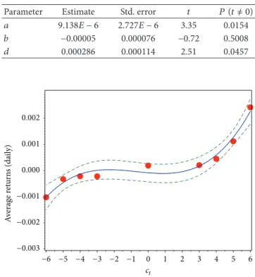
Figure 2 shows the relation between the average daily return of low-risk asset and the proxy of the excess demand for stock index (𝑐𝑡) and it gives some suggestions about the possible analytical expression to link these two variables. The central part of the graph (i.e.,−3 ≤ 𝑐_𝑡≤ 3) is almost flat, but at the two sides (i.e.,𝑐_𝑡< −3, 𝑐_𝑡> 3) the graph shows a positive dependency.

A possible empirical model describing the previous rela-tionship can be the following polynomial function:

̃𝑟𝑏,𝑡= 𝑎𝑐𝑡−13 − 𝑏𝑐𝑡−1+ 𝑑 + 𝜀𝑏,𝑡, (9) where ̃𝑟_𝑏,𝑡 are the daily returns observed for the Treasury bond and 𝑎 > 0, 𝑏 and 𝑑 are shape parameters to be estimated through a regression analysis which minimizes the error term. These estimates are shown inTable 1along with their significance test. Parameter 𝑎, which is relevant to characterize the polynomial model, appears significant at 1% confidence. Overall the regression has an adjusted determination coefficient (𝑅2) equal to.8824 and a value of the Root Mean Squared Error (RMSE) equal to.000341.

Table 1: Results of the regression analysis on the daily return observed: parameter estimates, standard error of the estimates,

Student’s𝑡 and probability of rejection.

Parameter Estimate Std. error 𝑡 𝑃 (𝑡 ̸= 0)

𝑎 9.138𝐸 − 6 2.727𝐸 − 6 3.35 0.0154 𝑏 −0.00005 0.000076 −0.72 0.5008 𝑑 0.000286 0.000114 2.51 0.0457 A verag e r et u rn s (da il y) −6 −5 −4 −3 −2 −1 0 1 2 3 4 5 6 ct −0.003 −0.002 −0.001 0.000 0.001 0.002

Figure 2: Relationship between the proxy variable of excess demand

(𝑐_𝑡) and the average daily returns on the US Treasury 30 years’ bonds

(red dots: observation period 1993–2008).𝑐_𝑡is calculated on data of

an NYSE stock index.

The continuous line inFigure 2represents the expression of̂𝑟_𝑏,𝑡in system(6), where the values of the parameters𝑎 and 𝑏 are fixed as inTable 1. WhatFigure 2shows is that the two markets (i.e., stocks and bonds) strengthen their link when a clear “sentiment” in the stock market persists. Indeed, when the returns of the NYSE have all the same sign during a week, the returns on the long-term bond move substantially away from zero and show the same sign as well.

4. Transition Dynamics

The analysis of the model dynamics can be developed by simulating the behavior of system(6)starting from different initial values of the excess demand. We consider here two levels for the initial excess demand: large and close to zero. We additionally combine these two cases with two different market configurations: one where rational investors prevail and the other where irrational investors (of the contrarian kind) prevail. Overall we therefore analyse four scenarios.

To check the internal consistency of the model we compare two types of correlations, which we call here ex-ante and ex-post. We refer to the ex-ex-ante correlation as the correlation estimated by rational agents through (4) and call ex-post correlation that resulting from the simulation of model(6). Of course, for the model to be consistent, the two types of correlations should take similar values under

(5)

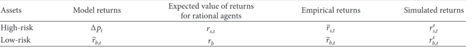
Table 2: Different types of returns.

Assets Model returns Expected value of returns

for rational agents Empirical returns Simulated returns

High-risk Δ𝑝_𝑡 𝑟_𝑠,𝑡 ̃𝑟𝑠,𝑡 𝑟𝑠,𝑡𝜀

Low-risk ̂𝑟_𝑏,𝑡 𝑟_𝑏 ̃𝑟𝑏,𝑡 𝑟𝜀𝑏,𝑡

Table 3: Correlation between the returns of high-risk and low-risk assets estimated by rational agents (ex-ante correlation).

Initial excess demand

Prevalence in the market Rational investors Contrarian speculators

𝜒₂= 30, 𝜒₁= 0.5 𝜒₂= 3, 𝜒₁= −4

Largely high or low 0.998 0.112

Close to zero 0.000 0.113

the same conditions. To obtain the estimate of the ex-post correlation, we simulate the returns of the two assets (i.e.,𝑟_𝑠,𝑡𝜀 and𝑟_𝑏,𝑡𝜀 ). These returns have been obtained adding a random disturbance toΔ𝑝_𝑡and tô𝑟_𝑏,𝑡, respectively, as described in the following equations:

𝑟_𝑠,𝑡𝜀 = Δ𝑝𝑡+ 𝑒𝑠,𝑡,

𝑟_𝑏,𝑡𝜀 = ̂𝑟_𝑏,𝑡+ 𝑒_𝑏,𝑡, (10) where𝑒_𝑠,𝑡and𝑒_𝑏,𝑡are i.i.d. disturbances distributed with zero expected value and standard deviations, respectively, equal to 0.02 and 0.00002.Table 2summarizes the different types of returns used. The purpose of adding a random disturbance is that of reducing the effect of purely deterministic simulation, where correlation between the two variables would be either 1 or−1.

The ex-post correlation on the returns simulated by model(6)is then calculated with the standard formula:

cov(𝑟_𝑠,𝑡𝜀 , 𝑟_𝑏,𝑡𝜀 ) 𝜎 (𝑟𝜀

𝑠,𝑡) 𝜎 (𝑟𝜀𝑏,𝑡)

, (11)

where cov(⋅, ⋅) and 𝜎(⋅) are, respectively, the usual covariance and standard deviation functions.

Tables3and4show the values of the correlation (resp., ex-ante and ex-post) between the returns of the two assets in the four scenarios.

Comparing the two Tables we can conclude that ex-post and ex-ante correlations change accordingly. Observing

Table 3, the large value of the ex-ante correlation occurs when rational agents dominate the market and the level of the excess demand gets very large. As already discussed, under these settings, rational agents estimate that the correlation between the traded assets (based on(4)) will run to unity. On the contrary in all the other combinations the ex-ante correlation estimate keeps at zero or slightly higher. Similar conclusions obtain observingTable 4.

Table 4: Correlation between the returns of high- and low-risk assets resulting from the simulation of the model (ex-post correlation).

Initial excess demand

Prevalence in the market Rational investors Contrarian speculators

𝜒2= 30, 𝜒1= 0.5 𝜒2= 3, 𝜒1= −4

Largely high or low 0.971 0.001

Close to zero 0.064 0.207

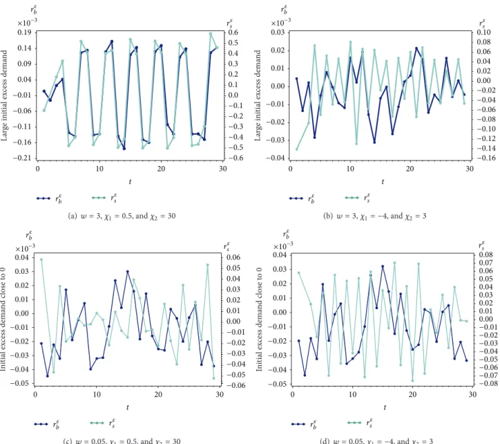
Figure 3shows simulated trajectories of𝑟_𝑠,𝑡𝜀 (light color) and 𝑟𝜀_𝑏,𝑡 (dark color). The cases where the initial excess demand is large are in the first row (panels (a) and (b)) and those where the initial excess demand is close to 0 are in the second row (panels (c) and (d)). Those trajectories have been obtained under the same setting that have been used for the estimate ofTable 4.

The visual inspection of Figure 3 confirms the results shown in Table 4. However the same figure also suggests to us something about the dynamics at the origin of the ex-post correlation. It is known that the theoretical model in (3) has a stable equilibrium in 𝑤_𝑡 = 0 and 𝑟_𝑠,𝑡 = 0. Indeed observing the second row ofFigure 3when the initial excess demand is sufficiently close to zero, the returns show a low correlation both when rational agents prevail and when speculators prevail. Things change significantly if the initial excess demand is very large and rational agents dominate, which is the case analyzed in panel (a). It is clear in this case that the system enters into an orbital dynamic, where the returns of both assets oscillate in a synchronous way. Indeed large positive values of the excess demand sustain large returns of both the risky and the low-risk assets, following, respectively,(2)and(9).

The model explains why both returns revert severely and turn to negative. When the price of the risky asset is high enough and combines with large excess demand, rational agents change deeply their portfolio as a consequence of two circumstances:

(i) mean reversion of prices generates highly negative expected returns (see(1));

(ii) large excess demand generates high correlation esti-mate, which in turn reduces the opportunity to form “balanced” portfolio, as it turns out from equation

(A.2) in the Appendix which determines the port-folio weight of the risky asset as a function of the

(6)

L ar ge ini tial ex cess dema n d −0.21 −0.16 −0.11 −0.06 −0.01 0.04 0.09 0.14 0.19 ×10−3 −0.6 −0.5 −0.4 −0.3 −0.2 −0.1 0.0 0.1 0.2 0.3 0.4 0.5 0.6 0 10 20 30 r𝜀b rs𝜀 r𝜀b r𝜀 s t (a)𝑤 = 3, 𝜒1= 0.5, and 𝜒2= 30 L ar ge ini tial ex cess dema n d −0.04 −0.03 −0.02 −0.01 0.00 0.01 0.02 0.03 ×10−3 −0.12 −0.10 −0.16 −0.14 −0.08 −0.06 −0.04 −0.02 0.00 0.02 0.04 0.06 0.08 0.10 0 10 20 30 rb𝜀 rs𝜀 r𝜀b r𝜀 s t (b) 𝑤 = 3, 𝜒1= −4, and 𝜒2= 3 In it ial ex ces s dema nd c los e t o 0 −0.05 −0.04 −0.03 −0.02 −0.01 0.00 0.01 0.02 0.04 0.03 ×10−3 0 10 20 30 r𝜀 b r𝜀s r𝜀 b t −0.06 −0.05 −0.04 −0.03 −0.02 −0.01 0.00 0.01 0.02 0.03 0.04 0.05 0.06 r𝜀s (c) 𝑤 = 0.05, 𝜒₁= 0.5, and 𝜒₂= 30 −0.06 −0.05 −0.08 −0.07 −0.04 −0.03 −0.02 −0.01 0.00 0.01 0.02 0.03 0.05 0.04 0.06 0.08 0.07 r𝜀 s In it ia l ex cess dema nd c los e t o 0 −0.05 −0.04 −0.03 −0.02 −0.01 0.00 0.01 0.02 0.04 0.03 ×10−3 0 10 20 30 r𝜀 b r𝜀s r𝜀b t (d)𝑤 = 0.05, 𝜒₁= −4, and 𝜒₂= 3

Figure 3: Simulated trajectories of the risky and the low-risk assets. For all plots parameter values are𝛼₁= 0.02, 𝛼₂= 0.06, 𝜆 = 0.05, 𝑌 = 0.5,

𝑟𝑏 = 0, 𝑃 = 1, 𝑘 = 0.20, and 𝜇 = 0, 15. (a) Prevalence of rational investors (𝜒2 = 30) and lower importance of momentum speculators

(𝜒₁= 0.5); (b) prevalence of contrarian speculators (𝜒₁ = −4) and lower importance of rational investors (𝜒₂ = 3). (c) and (d) Showing the

same market composition as in (a) and (b), but the starting value of the simulation is𝑤 = 0.05.

excess demand. Besides, extremely imbalanced port-folios are the expected result following the standard Markowitz theory when correlation between the asset values tends to 1.

Under such conditions, rational agents put on the market large order for selling the risky asset, and if they represent the large majority of the market a large negative excess demand appears on the market. Both the risky and the low-risk asset returns are then driven down and now the story can repeat symmetrically. If on the contrary rational agents do not dominate the market as in panels (b) and (d) ofFigure 3, then

their weight is not enough to condition the market and the orbit does not develop.

The core of the model lies in that rational investors antic-ipate the correlation breakdown of the asset returns. When they do, they react directing (almost entirely) their demand towards one of the two assets and getting rid of the other. Rational agents therefore successfully anticipate the correla-tion breakdown between the assets, but doing so they also destroy the portfolio diversification usually protecting their investment during standard market periods. The model pre-dicts also that when the market is sufficiently balanced with contrarian speculators, the (ex-post) correlation coefficient

(7)

remains at low levels, because they counterbalance the pro-cyclical behavior of rational investors.

5. Conclusions

The major point of this work has consisted of pushing forward the analysis of the model proposed by Falbo and Grassi [15]. Results have shown that the model is consistent with respect to the hypothesis that rational agents modify correctly their estimates of the variance and the covariance of the assets returns, anticipating the market excess demand. The relevance of this finding is in turn that of showing that putting on the shoulders of speculators all the responsibility for generating the financial crisis or the speculative bubbles, which occasionally occur on the financial markets, is not entirely justified. Indeed also risk averse, informed, rational investors can trigger such phenomena if they simply believe that large market consensus (such as large values of the excess demand) has an impact on the forthcoming correlation between the financial assets.

In extremely simplified terms this analysis has shown that also rational investors can be victim of a self-fulfilling prophecy, as soon as they attempt to anticipate what the mar-ket is going to do, which is usually attributed to speculators. Attributing to only speculators the origin of financial disas-ters is therefore not a correct way to understand such kind of events. Paradoxically we show that contrarian speculators act on the market as a countercyclical factor. The attitude of taking a given position on the market as a consequence of the fact that the large majority is doing the same appears

rather as the triggering factor. No superior information, no diversification, and no risk averse attitude seem to supply a sufficient antidote against it.

We assumed a model for the returns of the low-risky asset, whose analytical properties capture the fundamental features observable from the financial data. This is relevant because it adds an empirical consistency to the model, next to the theoretical one discussed above.

Appendix

We shortly remind the solution of the portfolio optimization for rational agents. We refer to Falbo and Grassi [15] for a detailed explanation of computation.

The optimal quantity 𝑞∗_𝑡 is obtained by searching the maximum of the following performance indicator:

𝑔 = q𝑇𝑡r

q𝑇

𝑡𝑉𝑡−1q𝑡,

(A.1)

wherer𝑇= [𝑟_{𝑠,𝑡−1} 𝑟_𝑏] is the vector of expected returns of the higher and low-risk assets andq𝑇_𝑡 = [𝑞_𝑡 1− 𝑞_𝑡] is the vector of their portfolio weights.

The variance-covariance matrix 𝑉_𝑡−1 is estimated as function of 𝑤_𝑡−1 referring to (4). 𝑔 is equivalent to the Sharpe ratio, so that the optimal portfolioq∗_𝑡 = arg max 𝑔 is also Markowitz efficient. The solution of the portfolio optimization problem, depending on the dynamic variables 𝑟_𝑠and𝑤, is the following:

𝑞∗ 𝑡 (𝑤𝑡−1, 𝑟𝑠,𝑡−1) = { { { { { { { { { { { { { { { − 𝑟𝑏 𝑟_{𝑠,𝑡−1}− 𝑟_𝑏+ √(𝛼2 1+ 𝛼22+ 2𝛼1𝛼2(𝑒−𝜇𝑤2𝑡−1− 1)) ((𝑟_{𝑠,𝑡−1}𝛼₂− 𝑟_𝑏𝛼₁)2+ 2𝛼₁𝛼₂𝑟_𝑏𝑟_{𝑠,𝑡−1}𝑒−𝜇𝑤𝑡−12 ) (𝑟_{𝑠,𝑡−1}− 𝑟_𝑏) (𝛼2 1+ 𝛼22− 2𝛼1𝛼2(−𝑒−𝜇𝑤2𝑡−1+ 1)) if 𝑟𝑠,𝑡−1 ̸= 𝑟𝑏 𝛼₁𝛼₂(−𝑒−𝜇𝑤2 𝑡−1+ 1) − 𝛼2 2 2𝛼₁𝛼₂(−𝑒−𝜇𝑤2 𝑡−1+ 1) − 𝛼2₁− 𝛼2₂ if 𝑟𝑠,𝑡−1= 𝑟𝑏. (A.2)

From(A.2),𝑞_𝑡∗(0, 𝑟_{𝑠,𝑡−1}) can be easily obtained as 𝑞∗_𝑡 (0, 𝑟_{𝑠,𝑡−1}) = − 𝑟𝑏 𝑟_{𝑠,𝑡−1}− 𝑟_𝑏+ √𝑟2 𝑠,𝑡−1𝛼22+ 𝑟𝑏2𝛼21 (𝑟_{𝑠,𝑡−1}− 𝑟_𝑏) √𝛼2 1+ 𝛼22 . (A.3)

Conflict of Interests

The authors have no conflict of interests related to publishing this paper.

References

[1] E. Bertero and C. Mayer, “Structure and performance: global interdependence of stock markets around the crash of October

1987,” European Economic Review, vol. 34, no. 6, pp. 1150–1180, 1990.

[2] M. A. King and S. Wadhwani, “Transmission of volatility between stock markets,” Review of Financial Studies, vol. 3, pp. 5–33, 1990.

[3] S. Calvo and C. Reinhart, “Capital flows to latin america: is there evidence of contagion effects?” in Private Capital Flows to Emerging Markets After the Mexican Crisis, G. A. Calvo, M. Goldstein, and E. Hochreiter, Eds., Institute for International Economics, Washington, DC, USA, 1996.

[4] T. Baig and I. Goldfajn, “Financial market contagion in the Asian crisis,” IMF Staff Papers, vol. 46, no. 2, pp. 167–195, 1999. [5] F. M. Longin, “The asymptotic distribution of extreme stock

(8)

[6] P. Hartmann, S. Straetmans, and C. G. de Vries, “Asset market linkages in crisis periods,” The Review of Economics and Statis-tics, vol. 86, no. 1, pp. 313–326, 2004.

[7] K.-H. Bae, G. A. Karolyi, and R. M. Stulz, “A new approach to measuring financial contagion,” Review of Financial Studies, vol. 16, no. 3, pp. 717–763, 2003.

[8] L. Ramchand and R. Susmel, “Volatility and cross correlation across major stock markets,” Journal of Empirical Finance, vol. 5, no. 4, pp. 397–416, 1998.

[9] A. Ang and G. Bekaert, “Regime switches in interest rates,” Journal of Business & Economic Statistics, vol. 20, no. 2, pp. 163– 182, 2002.

[10] F. Chesnay and E. Jondeau, “Does correlation between stock returns really increase during turbulent periods?” Economic Notes, vol. 30, no. 1, pp. 53–80, 2001.

[11] M. Loretan and W. B. English, “Evaluating correlation break-downs during periods of market volatility,” WP 658, Board of Governors of the Federal Reserve System International Finance, 2000.

[12] G. A. Karolyi and R. M. Stulz, “Why do markets move together? An investigation of U.S.-Japan stock return comovements,” The Journal of Finance, vol. 51, no. 3, pp. 951–986, 1996.

[13] B. H. Boyer, “Pitfalls in tests for changes in correlations,” International Finance Discussion Paper, Board of Governors of the Federal Reserve System, 1997.

[14] R. Rigobon, “Contagion: how to measure it?” in Preventing Currency Crises in Emerging Markets, S. Edwards and J. Frankel, Eds., pp. 269–334, The University of Chicago Press, Chicago, Ill, USA, 2001.

[15] P. Falbo and R. Grassi, “Market dynamics when agents antici-pate correlation breakdown,” Discrete Dynamics in Nature and Society, vol. 2011, Article ID 959847, 33 pages, 2011.

(9)

Submit your manuscripts at

http://www.hindawi.com

Hindawi Publishing Corporation

http://www.hindawi.com Volume 2014

Mathematics

Journal of

Mathematical Problems in Engineering

Hindawi Publishing Corporation http://www.hindawi.com

Differential Equations International Journal of

Volume 2014 Hindawi Publishing Corporation

http://www.hindawi.com Volume 2014 Hindawi Publishing Corporationhttp://www.hindawi.com Volume 2014

Mathematical PhysicsAdvances in

Complex Analysis

Journal of

Optimization

Journal of Hindawi Publishing Corporation

Combinatorics

International Journal of Hindawi Publishing Corporation

Journal of

Function Spaces

Abstract and Applied Analysis

http://www.hindawi.com Volume 2014 International Journal of Mathematics and Mathematical Sciences

Hindawi Publishing Corporation http://www.hindawi.com Volume 2014

The Scientific

World Journal

Discrete Dynamics in Nature and Society

Discrete Mathematics

Journal of

http://www.hindawi.com Volume 2014 Hindawi Publishing Corporationhttp://www.hindawi.com Volume 2014

Does Expectation of Correlation Breakdown in Financial Market Fulfill Itself?

Research Article