Identification of editing effect in image sequences by statistical modeling

Identification of editing effect in image sequences

by statistical modelling

N. Adami & R. Leonardi

Dept. of Electronics for Automation - University of Brescia

Via Branze 38, I-25123 Brescia - Italy

Phone +39-30-3715.434

E-mail:

{adami, leon}@ing.unibs.it

January 12, 2010

This work has been partially supported by project ESPRIT 28798 AVIR and the italian Ministry of the University and of the Scientific and Technological Research. The authors thank the Radio Televisione Italiana (RAI) for providing test material for the simulations.

Abstract

This paper presents a novel approach for video editing effect detection in digital image se-quences such as movies, commercials... The proposed method is based on histogram information and the decision criterion is derived from statistical properties of dissolve or wipe images, with respect to some hypothesis on the histograms of shots that surround the dissolve interval. More in particular the histogram of a dissolve image is given by the convolution of the histograms of two contiguous shots, provided that the random processes associated with the two shots are sta-tistically independent. A two step algorithm is presented: in the first step the dissolve effects are detected while in the second a precise estimate of the editing effect time interval is established. Simulation results indicate that high performance can be achieved with the proposed approach.

1

Introduction

An image sequence is formed of a certain number of shots that correspond to a series of frames typically extracted from a single camera record. During the editing stages, each camera record is linked to another one by means of editing effects such as cuts which simply define a sharp transition, wipes which corresponds to a sliding window effect, mates which let a dark blob invade the frames and dissolves, which represent a gradual change from one camera record to another by simple linear combination of the frames involved in the dissolve process. The weights of the linear combination are set on the basis of the distance of the frame which is part of the dissolve with respect to the beginning and the end of the surrounding shots respectively. Other effects such as fade-in and fade-out are also used; in the first case, it simply correspond to a dissolve from a continuous black shot to a real camera record, while in the second case, a camera record is progressively darkened.

A first attempt to temporally segment a video sequence is performed by identifying the single shots, i.e. by recovering the various editing effects. This is very relevant as the temporal organization of shots has often a semantic significance, which may be used to recover high-level descriptors of the audio-visual data. Once the shots have been separated, it is also possible to summarize the information content by the use of indices such as K-frames or video objects (mosaics/sprites). Such indexing procedure may be then efficiently used for subsequent queries [3].

As some of the editing effects such as dissolves have more semantic significance than others, it is also important to recover the type of editing being used. Depending on the type of audio-visual material, some editing effects may be used more than others. For example, a football game is likely to contain only cuts, whereas the situation is quite different for movies.

The automatic identification of editing effects has already been studied in the literature [1]. Most of the effort has been devoted to the identification of abrupt transitions between shots. Most approaches operate by measuring differences of color histograms. The performance of such algorithms when aiming to detect gradual transitions such as dissolves have not been very satisfactory [2].

Even though the approach proposed in this work falls under the category of histogram based methods, it reaches much better performance, as it relies on reasonable statistical models of shots and of the processing that takes place during the editing effect. The identification of the dissolve is achieved in two stages: the first one is a detection process, while the second aims at locating with precision the time interval that the editing effect is covering.

2

Statistical model

It is assumed that a dissolve is created by overlapping two camera records for the duration of the dissolve and by weighting the contribution of each frame at any given instant n on the basis of its location with respect to the boundaries of the editing effect. If the two overlapping shots are identified as shotprev and shotnext, the following relationship holds when they overlap for n = nin..nout (see

Fig. 1): F[n] = nout− n nout− nin × Fin[n] + n− nin nout− nin × Fout[n] (1)

At times, it is possible to have also a non linear combination of weights in the formation of the dissolve frame F [n]. The model that is proposed here after could be adopted accordingly. Assuming that the series of frames forming each shot are outcomes of a same stationary random process (at least for first order statistics), an estimate of the marginal pdf of each process is represented by the last frame of shotprev/shotnext prior to the dissolve, Fin/Fout, respectively.

w

n

Fin Fout

shotprev shotnext

n in n out n out n n in -- n -n_in n out - n in n out

Figure 1: Weighting behavior in presence of a dissolve.

Normally frames Fin and Fout are quite different so that it can be really assumed that their

associated histograms are those of two indipendent random variables. Accordingly for any frame F [n] being part of the dissolve, its associated first order statistics can be estimated by the convolution of the histograms Hin and Hout properly scaled to take into account the weighting factors contained in

Equation 1.

This implies that the difference between H[n] and Hin∗ Hout should ideally be zero. On the

contrary, if Fin and Fout belong to a same shot, the previous histogram difference would be different

from zero. From this simple consideration, it is possible to obtain a simple criterion for dissolve detection.

3

Dissolve detection method

The dissolve detection process tries to identify its central temporal location where ideally we should have: F = Fin+Fout

2 .

Consider now the following expressions:

H[n] = H1

2[n] ∗ H12[n]

HM[n] = H1

2[n − M ] ∗ H12[n + M ]

(2) where M > 0 is a parameter (which should ideally be set so as to correspond to slightly over half the duration of the dissolve and H1

2[n] is the histogram of a generic frame F [n] scaled by half (

1 2F[n]).

Now if one estimates the function:

R[n] = χ 2 (H[n], H[n]) χ2_{(H[n], H} M[n]) − 1 (3)

Assuming that n is the center of a dissolve and that M is set so that H(n − M ) = Hin and

H[n + M ] = Hout, the denominator of the fraction in function R[n] will be substantially smaller than

its numerator (and in an ideal situation, it would go to zero). On the other hand, if there are no dissolves, numerator and denominator of the same fraction will have substantially the same value (and in an ideal situation, the fraction would go to 1). In other words, in presence of a dissolve, R[n] exhibits local maxima (≫ 0), while in the other cases, R[n] is substantially zero or negative. The aforementioned criterion is preferable to the one based on searching the local minima of the function χ2_{(H[n], H}

M[n]). In this case, as no normalization is taking place with respect to the histogram

characteristics, false detection are more likely to occur. With the previous procedure, in presence of a dissolve, we have roughly found its central location, n. It is now necessary to estimate its extent. For this purpose the function D(d, n) is computed.

D(d, n) = χ2

(H[n], Hd[n]) (4)

The minimum of such function with respect to d correspond to the boundaries of the dissolve with respect to n, which are located at n − d and n + d.

4

Test and Results

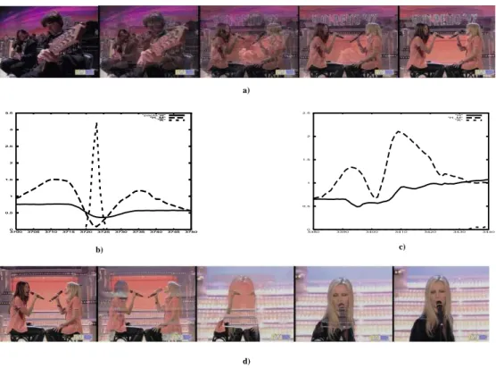
The algorithm has been tested extensively on various image sequences, demonstrating good perfor-mance both in terms of dissolve detection and precise estimation of their extent. Figure 3 shows an example of the R[n] function with real data, the parameter M being set to 15. Even if a low threshold is set, only two false detections are obtained. These occur typically because of the presence of shots with very short duration. They can be easily be removed by analyzing the monotonously decreasing behavior of the D[d, n] function (see Fig. 2). An alternative way to remove such false detections is to combine the result with the one of an abrupt transition detction algorithm. Another problem is the missed detection of a dissolve due to the statistical dependence of the histograms. The Figure 4 a) shows a dissolve for which the statistical independence hypothesis is correct and, as it can be seen by Figure 4 b), the correspondent R[n] exhibits a peak. This does not happen for the dissolve of Figure 4 c) and d) where the two shots are very similar.

130 140 150 160 170 180 190 0 2 4 6 8 10 12 14 16 18 20 D(d) 132 134 136 138 140 142 144 146 148 150 0 2 4 6 8 10 12 14 16 18 20 D(d) a) b)

Figure 2: Example of a typical D[d, n].

In a) the function D[d, n] is shown in presence of a real dissolve, while in b) the same function is shown for a false first step detection, in presence of very short shot durations.

0 10 20 30 40 50 60 70 80 0 100 200 300 400 500 600 700 R(n)

0 0.5 1 1.5 2 2.5 3 3.5 3700 37053710 3715 37203725 3730 37353740 3745 3750 "H" "H_M""R" 0 0.5 1 1.5 2 2.5 3 3.5 3700 37053710 3715 37203725 3730 37353740 3745 3750 "paola_0" "H_M""R" 0 0.5 1 1.5 2 2.5 3380 3390 3400 3410 3420 3430 3440 "H" "H_M""R" a) b) c) d) Figure 4:

Figure a) is a dissolve of two quite different shots and in b) are depicted the correspondents H,HM Rfunctions. In the same way Figures c) and d) are relative to a dissolve between similar shot

5

Conclusion

The proposed algorithm is based on a criterion which uses the hypotesis of statistical independence of the shots which are involved in creating the dissolve effect. The proposed algorithm establishes first the temporal location of the effect; then its extent is found by appropriate means. Extensive simulation results are showing good performance, both in terms of correct detection and no false alarms. The adopted statistical model can be applied not only to detect dissolve. It is accurate in all the cases where the transition image can be expressed as a linear combination of two random variables (e.g. wipe ..). Complex editing effects require further investigation whenever the transition image can be modeled as non linear combination of two random variables.

References

[1] J.S. Boreczky and L.A. Rowe. Comparison of video shot boundary detection techniques. Storage & Retrieval for Image and Video Databases IV, Proc. SPIE 2670:170–179, 1996.

[2] G. Lupatini, C. Saraceno, and R. Leonardi. Scene break detection: a comparison. Research Issues in Data Engineering, February 23-24 1998.

[3] C. Saraceno. Content-Based Representation and Analysis of Video Sequences by Joint Audio and Visual Information. PhD thesis, University of Brescia, 1998.