Inventory Management in Closed Loop Supply Chains: a heuristic approach with safety stock on demand

1

Inventory Management in Closed Loop Supply Chains:

a heuristic approach with safety stock on demand

Andrea Buccini (andrea.buccini@uniroma2.it)

Department of Management, “Tor Vergata” University of Rome, Italy

Massimiliano M. Schiraldi

Department of Management, “Tor Vergata” University of Rome, Italy

Erica Segel

Department of Management, “Tor Vergata” University of Rome, Italy

Abstract

Inventory management is one of the most important aspect in Closed Loop Supply Chain. This paper introduces a strategy for managing the return flow in order to increase service level in a stochastic scenario. We analyse a single-product hybrid system where inventory level is under continuous review and remanufacturing is used as a recovery option to protect from stockout. The aim is to exploit the opportunity of relocating safety stocks from a serviceable inventory to a remanufacturable inventory, in order to reduce stockholding costs.

Keywords: Inventory Management, Close Loop Supply Chain, Remanufacturing.

Introduction

Increased profitability, societal pressure, ethical responsibility, environmental legislation and asset (brand) protection are just some of the reasons for companies to engage in product recovery management. However, the integration of product recovery into logistics processes brings additional complexity to traditional operations management methodologies and practices and entails a transformation of the traditional Supply Chain Management, as we know it. From a logistics perspective, product recovery initiates additional goods flows from end users to original equipment manufacturer (OEM) or/and specialized companies. The management of these flows, opposite to the conventional supply chain flows, is addressed in the recently emerged field of “Reverse Logistics” (RL). Fleischmann et al., (1997) subdivided Reverse Logistics into three main areas, namely distribution planning, production planning and inventory control. The latter is where we put the focus of our contribution. Traditional inventory control models do not take into consideration that issued items, which the serviceable inventory due to customer demands, may be returned by the end-users after a certain time lag and recovered by the manufacturer. Thus, the adequacy and applicability of the traditional inventory management methods depends on two different aspects, namely the actors involved in the recovery activities and their respective

2

functions. Whereas specialized recycling companies purchasing used products and/or materials from third parties may possibly rely on traditional inventory control methods, the original equipment manufacturer (OEM) have to face a different situation where returned products may represent an alternative input resource in the manufacturing process. As a consequence, integrating the returning flows of the used products into the control strategy of the OEM requires the developing of appropriate mechanisms. In the recent years, inventory management in the reverse logistics context is been largely investigate and identified as a key area. Recoverable manufacturing systems can be defined as closed loop systems with discarded items used in place of externally supplied virgin materials to the extent possible in the fabrication of new products (Guide et al., 2000). These systems are capable of dealing with product returns via several product recovery options, e.g. direct reuse, repair, refurbishing, remanufacturing, cannibalization and recycling (Thierry et al., 1995). The objective for such hybrid systems with manufacturing and recovery processes is to control external component orders and the internal component recovery operations to guarantee a required service level and/or to minimize fixed and variable costs. Reviews of the related literature are provided by Guide et al. (1997), for repair models, and Fleischmann et al. (1997), for refurbishing/remanufacturing models. A more recent (remanufacturing) contribution is that by van der Laan et al. (1999). In addition to the theoretical contributions, case studies have been reported by Toktay et al. (2000), for single-use cameras, Rudi and Pyke (2000), for medical devices, van der Laan (1997), for automotive exchange parts and Fleischmann (2001), for electronic equipment. From an inventory control perspective most of the model that have been considered in the literature, have a fairly similar structure. Consequently, is possible to highlight a number of general observations. Figure 1 presents a general framework displaying the goods flows in case of products returns, which is adapted from Van der Laan (1997).

Figure 1. Framework of inventory system with Reverse Logistics

The producer has two distinct alternative suppliers in order to satisfy demand for new products. One is to follow the traditional scheme of ordering the required raw materials to en external supplier and fabricates new products, while the other is to overhauls old products and brings them back to “as new” conditions. However, the presence of returns certainly introduces an extra source of complexities into system interactions (such as the interaction between the output of the manufacturing and recovery processes, and the correlation between demands and returns) and return uncertainties (such as the uncertainty in the timing, quantity and quality of returned products). Clearly, these factors are not present in traditional systems. Finally, it should be noted that the logistics system, showed above, forms a link between two exogenous drivers, namely (recoverable) supply and demand. The relation between both processes appears to be one main discriminating factor characterising different recovery systems. As a matter of fact, product recovery models do not entail a priori assumptions on the type of relation

manufacturing remanufacturing _serviceable inventory customer returns inventory product demands product returns

3

between products demand and returns, where the latters are expected to be returned after a stochastic market sojourn time.

Considerations on the product life cycle

The current stage of a product’s life cycle is the first organizational strategic factor that influences the management of a supply chain of an organization. The typical product life cycle includes four phases (see, e.g. Kotler, 1995): a product introduction phase, which is characterized by increasing production capacity and logistics channels developing; a maturity phase, where process and cost efficiencies are typically implemented; a decline phase, where the focus is on product divestment. Clearly, is necessary to carefully evaluate the product life cycle phase impact on the greening of the supply chain.

A product life cycle view in a reverse logistics context.

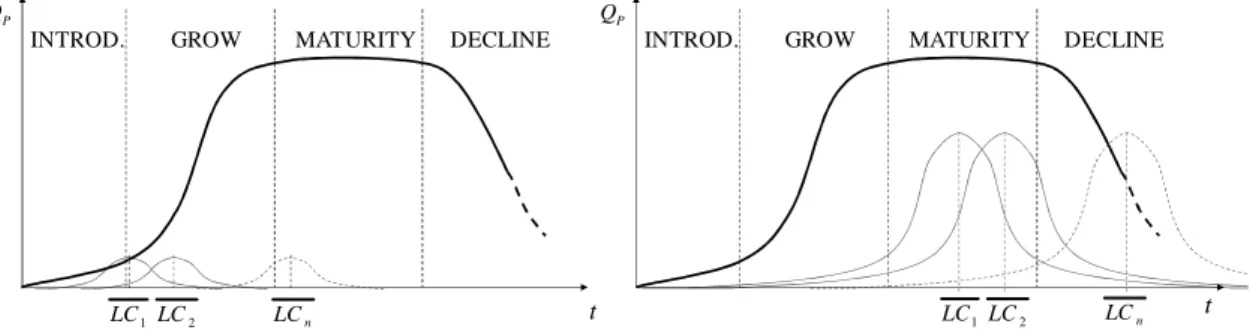
A proper observation and definition of the product life cycle is needed to estimate the expected return flow of products and thus determine the best inventory management policy that maximizes the benefits achieved by the integration of new and reusable product flow. A S-shaped curve it is typically adopted to define the life cycle of a product which indicates the number of units that are placed on the market and therefore to estimate the return rate based on the demand rate of a particular phase (Tibben-Lembke R.S, 2002). This approach does not take into account different types of products according to their actual stage in the life cycle, but considers only the production evolution over time and cannot distinguish goods with long life cycle (e.g. electronic/mechanical devices) from those with a short one (e.g. packaging). To our knowledge, no contribution made so far seems to include the (real) life cycle of the product in the return rate estimation.

We can distinguish three phases in the product life cycle (Jun H.B et al., 2007):

• Begin of Life (BOL): manufacturing and distribution

• Middle of Life (MOL): customer service and maintenance

• End of Life (EOL): disposal, reuse and recycle.

Therefore, we strongly suggest that the rate of return of the product should depend on its life cycle, and assume that the life of a product is related to a random normal variable Product_Life_Cycle = N

(

σ

)

Hence, we can represent the probability that a product ceases its normal use within a certain time during different phases, thus representing a potential return: e.g. fault for design or manufacturing (BOL), problems related to failure or and of use (MOL), obsolescence or usage (EOL).

Figure 2. A representation of the product lifecycle distribution t EOL MOL BOL LC ) (t f_LC

4

The different types of products result in different values of the mean life cycle and in their variability (standard deviation) and then different return rates along the to the S-shaped market curve.

Figure 3. Different product lifecycles determine different return rates over time

However, a detailed estimation of the return rate is beyond the scope of this paper. Thus, to our extent, we assume the return rate to be constant and equal to its mean value, which is reasonable in the case of reusable packages.

A Lot-sizing policy

To set the foundations of this study, we begin by addressing the lot sizing problem. We adopt a heuristic procedure for approximating optimal order quantities, exploiting the logic of the Economic Order Quantity (EOQ), as its been presented by van der Laan and Teunter (2006). Heuristic approaches have important practical value; they are easier to understand and to implement, and are generally preferred in practice. The main advantage of EOQ models is that, due to their simplicity, they lead to closed-form expressions for the optimal batch sizes. Unfortunately, the strong underlying assumptions are often not too realistic. However, following the same approach as in traditional inventory systems with manufacturing only, the EOQs can be used as approximations of more realistic situations.

Hybrid systems are the answer to a growing need for integrating environmentally sound choices into inventory control management. However, it is not just only about being environment friendly, it is about business opportunity and increasing profits. In fact, the expected total costs of implementing a hybrid system may be potentially lower than the traditional system without recovery options. This is mainly due to saves in material costs as a result of the re-use of items. These cost savings may make it cheaper to recover a used product than to manufacture a completely new product (van der Laan et al., 1999). Unfortunately hybrid systems have to face various sources of uncertainty (such as the uncertainty in the timing, quantity and quality of returned products) that are absent in traditional manufacturing systems. Clearly, in order to control such a system efficiently, manufacturing and remanufacturing decisions have to be coordinated.

In this paper, we analyse a single-product hybrid system where remanufacturing is used as the recovery option and we assume the inventory level is under continuous review. In addition to newly produced items, remanufactured items as well can be used to meet customer demands. Remanufactured products are considered to be as-good-as-new, but remanufacturing occurs to be cheaper than manufacturing. Hence can lead to considerable costs savings. What we focus on the phase where, due to the maturity of the design, we aspect the returns to be a sufficient to set up a remanufacturing operation.

P Q t MATURITY DECLINE GROW INTROD. 1 LC LC2 LCn P Q t MATURITY DECLINE GROW INTROD. 1 LC LC2 LCn

5

Within this perspective, we consider manufacturing to be trigger by a standard re-order level (RL) policy with EOQ. In PUSH control, the timing of the remanufacturing operations is completely return driven: as soon as sufficient returned products are in the returns inventory, these products are batched and pushed into the remanufacturing process. On the other hand, with PULL control, the timing of the remanufacturing operations depends on a composite of returns, future expected demands, and inventory positions. Informally, under PUSH control, remanufacturing operations are scheduled as early as possible, whereas under PULL control they are scheduled as late as is convenient.

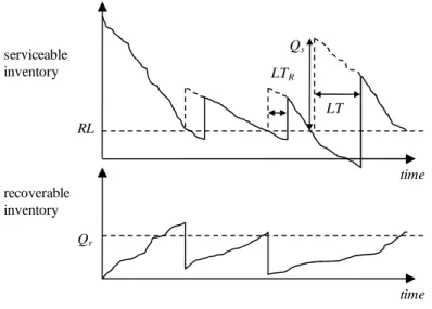
PULL policies prevent large stocks by using an order level for remanufacturing, while PULL strategy outperforms the PUSH strategy when stockholding costs for returned products is lower than that of remanufactured products (van der Laan et al., 1999). Henceforth, pull strategy is further analysed. This is illustrated in Figure 4.

Figure 4. An example of PULL policy

The heuristic solution provided by van der Laan et al., allows a simple computation of the EOQ in serviceable and return inventory, despite not introducing a planning horizon in the EOQ formulation. Thus it can be modified as follows:

s r m m h d r h d r P r d K Q ) -1 ( + ) -( 2 = s r r r h d r h P r K Q + 2 = Where:

• Km and Kr are respectively the fixed order and remanufacturing cost

• d and rare respectively the mean demand and return rate (i.e. daily or weekly)

• h and s hr are respectively the unit holding cost for new and returned items per

time unit (i.e. day or weeks)

• P the planning horizon (number of time units, i.e. number of days, weeks)

LT LTR Qr RL Qs time time serviceable inventory recoverable inventory

6

A strategy to increase the service level through remanufacturing

In a stochastic scenario we are forced to take into account demand and lead time variability in order to assure a desirable service level. A major limit of van der Laan and Teunter’s model is to consider backorder costs, which are well known to be very difficult to estimate in real contexts: thus, we prefer to adopt a different approach focused on setting target service level. In the remainder of this paragraph we address this issue in more detail. Subsequently, we modify the model introducing a service level objective and we extend the analysis to allow for stochastic lead-times based on the Hadley and Whitin safety stock model (1963). When inventory availability is measured in terms of the no-stock out probability per order cycle and the traditional safety factor (k) approach to setting safety stocks levels is employed, safety stocks are a function of the management specified service level and the standard deviation of demand during delivery time. The customer service level is in this way translated into a safety stock level, which is physically made available in the warehouse. Therefore, we propose a method to control external component orders and the internal component recovery process to guarantee a required service level. In our model we consider a re-order level (RL) inventory policy and assume customer demand and procurement delivery time to be independent random variables, so that:

1. The demand follows a normal distribution, N(d,σD)

2. The procurement delivery follows a normal distribution, N(LT,σLT) 3. The remanufacturing lead time follows a normal distribution ( , )

R

LT

R σ

LT N

The following notation will be used:

A strategy for including the reverse flow in safety stocks

The objective is to exploit the opportunity of relocating safety stocks (SS) from the serviceable inventory to the remanufacturable inventory, in order to reduce the inevitable inventory costs, which are entailed by maintaining SS in the warehouse. Since the strategy is based on the possibility to launch the order for safety stock as late as convenient, hence only when is required to assure the desired service level, a fundamental condition must be satisfied:

LT ST LTR + R <

Table 1 – Notation

D stochastic demand rate with mean dand standard deviation σD R stochastic return rate with mean rand standard deviation σr

LT stochastic procurement lead time with mean LTand standard deviation σLT LTR stochastic remanufacturing lead time with mean LT_Rand standard deviation

R

LT

σ

InvT inventory level at the time T T

SO

T minimum time to stock out event at the instant T SSm safety stock of serviceable items

7

That is the remanufacturing lead time (i.e. remanufacturing average lead time plus a safety time determined on the basis of a confidence value) is generally lower than the mean procurement lead time.

STR =krσLT_R is the safety time for LTR and kr is defined as value confidence dx x f s k _ ) ( 2 1 -=

∫

π

For example, to be confident at 99% that the total remanufacturing time will be lower than procurement lead time, kr should be not lower than 2.33. As previously stated, we

also assume that:

hr < hs

The inventory observation period starts from the moment when the stock level drops under the re-order level RL, and ends the moment when a batch from the supplier or the remanufacturing is received, thus traditionally:

d

RL= LT

Since in our paper we consider a PULL reorder policy, we should define a minimum level of safety stock in the serviceable inventory in order to protect from the variability during the stochastic remanufacturing lead time. Furthermore, we should consider an extra safety stock level in the returns inventory during the procurement lead time. Safety stock level under remanufacturing lead time

In this section, we compute the minimum SS level necessary to cope with demand and lead time variability, while a remanufacturing pending order is been launched in the serviceable inventory. According to Hadley and Whitin formula, we obtain:

R D LT m k d σ σ LT SS R 2 2 2 + =

Where k is the dimensionless safety factor relating the investment in safety stock to measure of service level (SL):

SL dx x f k =

∫

π

LT d k SS_m < 2σ_LT2 +σ_D2 if 2 2 2 2 + ) -( < d σ d LT LT σ σ D R LT LT_R

8

remarking the hypothesis LTR < LT, this can be reduce to

2 2 + ) -( < D R LT LT RSD LT LT σ σ R

Where RSDD indicates the variation coefficient of the demand.

Safety stock level under procurement lead time

During the procurement lead time, since we assumed LTR <LT , we face the demand and lead time variability in a longer time span, thus an extra safety stock level is necessary to be held in the remanufacturing inventory. Therefore, it is necessary to choose when to place the order and how many items are required. An heuristic approach is here proposed.

As shown in Figure 5, we define a confidence interval in which the demand will fluctuate with probability pD and we define α, αM, αm, the mean, the maximum and the minimum demand curve slope respectively, that are:

= α _arctg( d 1 ) ; α_M =_arctg( D Dσ k d + 1 ); αm =arctg( D Dσ k d -1 ) being kD so that +0,5 2 = ) ( 2 1

∫

As a result, at a generic time t within the time span from the moment the inventory level drops under the RL to the moment when the order is delivered, assuming that in the worst case the demand slope would not exceed αM _{(as shown in} Figure 5), we obtain

that we should not incur in stock out before:

= + ) ( = _{Inv tg} α T T T M T SO T σ k d InvT D D + +

Consequently, the strategy operates iteratively evaluating, at each instant T, whether to order the units at this time or to postpone the decision to ∆T (i.e. to the next time T+1). The decision will be taken at the time T* when the following condition is met:

LT

T -

(

)

The number of units to remanufacture at the instant T* depends on the inventory level at this time. Since we want to grant service level SL, we have to consider the demand and lead time variability starting from the instant T* to LT. Therefore, if the inventory level at the time T* is Inv_T*a simple heuristic may return the SSr order size as:

= r SS _{k d}2σ2 +σ2(LT-T*) D LT -( - ( - )) * * d LT T Inv_T Where (Inv * -d(LT -T*))

T is the gap between the inventory level at the time T

*

and the expected average inventory at that time. In this way, if the actual demand sticks to its

9

average and, thus, at T* the inventory level is exactly equal to the expected, the SSr

order size returns the original Hadley & Whitin formula, computed on the remaining *

- T

LT time before the arrival of the replenishment lot, that is: = r SS _{k d}2σ2 +σ2(LT -T*) D LT

The proposed strategy becomes economically feasible if the following condition is satisfied: s r r r s r MIN SO r SS h SS h LT h SS T LT K + ( - ) + ≤ that is ≤ ⋅ −φ LT T h h MIN SO s r where r r SS K =

φ is the remanufacturing cost for one unit of safety stock.

Figure 5. Confidence range of the demand rate

Conclusions

In this paper an heuristic inventory management approach has been discussed in order to integrate the new and returned item flows in a stochastic scenario. Staring from the literature analysis, we observed that there are few contributions on safety stock computation in a reverse logistics scenario, with the objective to grant a desired service level despite minimizing a cost function that includes backorder costs. A safety stock policy has then been introduced, together with its economical evaluation, to exploit the opportunity to relocate safety stock to remanufacturable warehouse. Based on the continuous inventory level review, a simple heuristic allows to identify the proper time to place the necessary safety stock order from the recovery inventory, thus replenishing the serviceable inventory just in time and just in case. Starting from this contribute a further research is needed to deepen the analysis in order to study how to include the products lifecycle in their return rate estimation.

LT MIN SO T R ST Q time α m α M α * T R LT 0

10 References

Fleischmann M., Bloemhof-Ruwaard J.M., Dekker R., van der Laan E., van Nunen J.A.E.E. and van Wassenhove L.N., “Quantitative models for reverse logistics: A review”, European Journal of Operational Research, vol. 103, 1997, pp. 1–17.

Guide V.D.R., Jayaraman V., Srivastava R. and Benton W.C., “Supply-chain management for recoverable manufacturing systems”, Interfaces, vol. 30, 3, 2000, pp. 125–142.

Guide V.D.R., Jayaraman V., Srivastava R, “Repairablei nventory theory: Models and applications”, European Journal of Operational Research, vol. 102, 1997, pp. 1–20.

Hadley G., Whitin T.M., “Analysis of Inventory Systems” Prentice Hall, Inc., Englewood Cliffs, N.J. 1963.

Jelinski L.W., Graedel T.E., Laudise W.D., McCall D.W. and Patel K.N., “Industrial ecology: concepts and approaches”, Proceedings of the National Academy of Sciences, vol. 89, 1996, pp. 793–797.

Jun H.B., Kiritsisa D., and Xirouchakisa P., “Research issues on closed-loop PLM”, Computers in Industry, vol. 58, 8-9, 2007, pp 855-868.

Kotler R.J., “Principles of Marketing”, 7th ed., Prentice-Hall International, Englewood Cliffs, NJ, 1995.

Lowe E., “Industrial ecology: an organizing framework for environmental management”, Total Quality Environmental Management, vol. 3, 1, 1990, pp. 73–85.

Rudi N. and Pyke D.F., “Product recovery at the Norwegian health insurance administration”, INTERFACES, vol. 30, 3, 2000, pp. 166–179.

Tibben-Lembke R.S., “The impact of reverse logistics on the total cost of ownership”, Journal of Marketing: Theory and Practice, 1999, pp. 51–60.

Tibben-Lembke R.S., “Life after death: Reverse logistics and the product life cycle”, International Journal of Physical Distribution & Logistics Management, 32, 3-4, 2002, pp. 223-244.

Thierry M., Salomon M., van Nunen J. and Van Wassenhove, L.N., “Strategic issues in product recovery management”, California Management Review, 37, 2, 1995, pp. 114–134.

Toktay L.B., Wein L.M. and Zenios S.A., “Inventory management of remanufacturable products”, Management Science, vol. 46, 11, 2000, pp. 1412–1426.

van der Laan E.A., Salomon M., “Production planning and inventory control with remanufacturing and disposal”, European Journal of Operational Research, vol. 102, 2, 1997, pp. 264–278.

van der Laan E.A., Salomon M., Dekker R., van Wassenhove L., “Inventory control in hybrid systems with remanufacturing, Management Science”, vol. 45, 5, 1999, pp. 733–747.

van der Laan E.A., Teunter R.H., “Simple heuristics for push and pull remanufacturing policies”, European Journal of Operational Research, vol. 175, 2006, pp. 1084–1102.