Review Article
A New Theory to Forecast the Price of
Nonrenewable Energy Resources with Mass and
Energy-Capital Conservation Equations
Fabio Gori
Department of Industrial Engineering, University of Rome “Tor Vergata,” Via del Politecnico 1, 00133 Rome, Italy
Correspondence should be addressed to Fabio Gori; [email protected] Received 31 December 2013; Accepted 1 April 2014; Published 5 June 2014 Academic Editors: K. Abhary and Y. Demirel
Copyright © 2014 Fabio Gori. This is an open access article distributed under the Creative Commons Attribution License, which permits unrestricted use, distribution, and reproduction in any medium, provided the original work is properly cited.
The mass and energy-capital conservation equations are employed to study the time evolution of mass and price of nonrenewable energy resources, extracted and sold to the market, in case of no-accumulation and no-depletion, that is, when the resources are extracted and sold to the market at the same mass flow rate. The Hotelling rule for nonrenewable resources, that is, an exponential increase of the price at the rate of the current interest multiplied the time, is shown to be a special case of the general energy-capital conservation equation when the mass flow rate of extracted resources is unity. The mass and energy-capital conservation equations are solved jointly to investigate the time evolution of the extracted resources.
1. Introduction
The price evolution of nonrenewable energy resources is a very important problem in an economy based on non-renewable energy resources. The economics of exhaustible
resources was investigated by Hotelling [1], and reviewed in
[2], with the conclusion that the price of a resource increases
exponentially with the product of time and interest rate of capital.
After the oil crisis of 1973 the problem of the energy resources became a very important issue and several energy models and forecasts have been developed and employed.
During the decade of 1970s, among the others, McCall [3]
presented a linear program for the world oil industry which
was employed by an oil company. Tewksbury [4] described
a practical general approach to forecast foreign oil prices
to the year 2000. Pindyck [5] described a new version of
an econometric policy model of the natural gas industry.
Adelman [6] forecasted a decade of rising real oil prices for
the US. DuMoulin and Newland [7] came to the conclusion
that a rapid take-off in demand is likely to be followed by a rapid increase in the price of oil.
During the 1980s, among the others, Pearce [8] presented
an overall look at the world energy demand forecasts with
the conclusion that the judgment, rather than explicit mod-elling, is used to suggest a world crude oil scenario in which
oil prices rise at 10% per year. French [9] discussed the
mar-kets of world oil, natural gas, coal, electricity, and the energy demand, with the conclusion that from mid-decade onward energy prices will most likely increase more rapidly than the
overall price level. Roberts [10] concluded his analysis that
through the mid-1980s, real crude prices should be flat to down and thereafter increase at a rate equal to or less than
inflation. Campbell and Hubbard [11] showed that forecasts
of prices—including oil, natural gas, equipment and drilling costs, and money—affect the evaluation of all projects. Clark
[12] focused on generalized price formation in the U.S. gas
industry. David and Carson [13] focused on the banks which
use the long term oil supply and demand situation as the underlying support for making oil and gas price projections.
Lorentsen and Roland [14] outlined a very open model, which
can easily impose different assumptions about oil supply and demand in order to indicate a range of feasible projections
for oil prices. Curlee [15] concluded that overall assessment
of forecasts and recent oil market trends suggests that prices will remain constant in real terms for the remainder of the 1980s, to increase by 2-3% during the 1990s and beyond.
Anon [16] studied the U.S. demand for petroleum products
Volume 2014, Article ID 529748, 37 pages http://dx.doi.org/10.1155/2014/529748
in 1987, based on the assumption that world oil prices will average 13 US $/bbl through the third quarter of 1986 and rise gradually to 18 US $/bbl by the end of 1987. Dielwart and
Coles [17] discussed the current market uncertainties and
their impact on Canadian oil and natural gas prices. Yohe
[18] presented an analytical technique based on an adaptive
expectations model of incorporating current information
into long-term forecast. Sekera [19] presented three price
forecasting analyses with forecasts under each theory and the recommendation that all long term forecasts be based on fundamental/economic analysis, while short term forecasting
needs to utilize other methods. Gately [20] reviewed recent
and current opinions about prospects for prices in the world market for crude oil with two alternative views. Holden et al.
[21] examined the accuracy and properties of forecasts by
the OECD for 24 countries and 8 variables. Dougherty [22]
presented some rules of thumb that may help to understand the evolution of oil prices, to identify factors to consider when deciding on the credibility of an oil price forecast, rather
than to prophesize future oil price. Amano [23] developed
an annual, small-scale econometric model of the world oil market to analyze oil market conditions and oil prices for the period 1986–1991.
During the 1990s, among the others, Garces [24] explored
the effects of natural gas storage on short-term gas price forecasts, with preliminary results which indicate that by using natural gas storage as a causal variable, the final gas price forecasts can decrease by as much as 5% over
the forecast period. Angelier [25] concluded his analytical
framework with the forecast that, in the year 2000, oil prices will not be significantly different from those of 1990s. Bopp
and Lady [26] concluded their analysis that when actual
prices are employed, future prices did correctly anticipate
the observed seasonal pattern. Abramson and Finizza [27]
developed a system that forecasts crude oil prices via Monte
Carlo analyses of the network. Charleson and Weber [28]
forecasted energy consumption in Western Australia with
Bayesian vector autoregressions to 2010. Fesharaki [29]
believed that for the next three to five years oil prices will remain at lower levels than generally predicted, because price increases, even when they occur, will not be sustainable
for very long. Huntington [30] reviewed forecasts of oil
prices over the 1980s that were made in 1980, identifying the sources of errors due to such factors as exogenous GNP assumptions, resource supply conditions outside the cartel, and demand adjustments to price changes. Moosa and
Al-Loughani [31], on the basis of monthly observations on spot
and future prices of the West Texas Intermediate (WTI) crude oil, suggested that future prices are neither unbiased nor
efficient forecasters of spot prices. Abramson [32] discussed
a knowledge-based system that models the crude oil market as a belief network and uses scenario generation and
Monte-Carlo analysis to forecast oil prices. Skov [33] reviewed some
of the more significant forecasts of energy supply, demand, and oil prices made in the last 25 years and identifies the basic premises used and why they led to incorrect forecasts.
Abramson and Finizza [34] described a case study in the
use of inherently probabilistic belief network models to produce probabilistic forecasts of average annual oil prices.
Santini [35] investigated the statistical model of oil prices
examining issues and trends related to both the U.S. and
world oil supply. Williams [36], in order to forecast the
future, examined historical trends and presents the new idea that there is an inverse relationship between crude oil prices volatility and the strength of the relationship between the owners of crude oil (host governments) and the oil companies that develop, refine, market, and sell the
products. Chaudhuri and Daniel [37] demonstrated that the
nonstationary behavior of US dollar real exchange rates, over the post-Bretton Woods era, is due to the nonstationary
behavior of real oil prices. Pindyck [38] discussed how price
forecasts also influence investment decisions and the choice
of products to produce. Silvapulle and Moosa [39] examined
the relationship between the spot and futures prices of WTI crude oil using a sample of daily data with the result that both spot and futures markets react simultaneously to new information.
During the 2000s, among the others, Alba and Bourdaire
[40] consider the actual situation as a “cohabitation” between
oil and the other energies with the oil price, extremely volatile, reflecting the trial and error adjustment of the market share left to the other energies. The Centre for Global Energy
Studies [41] covers several topics including oilfields set to
begin production in 2000, non-OPEC production, demand in western OECD countries and the Asia Pacific region, and oil
price forecasts. According to the US energy information [42]
global crude oil prices in 2000 will rise to 24 US $/bbl, up by 2 US $/bbl from its earlier estimate, while spot prices for West Texas Intermediate crude will average more than 22 US $/bbl
through 2001. Hare [43] reported that according to forecasts
by the Energy Information Administration, increases in natural gas prices will continue all the way to the summer and winter of 2000, and that high oil prices will still be seen in 2001. According to the managing director of Shell’s
exploration and production [44] crude oil prices will average
in the mid-teens of US $/bbl over the next 10 years. The Energy Department of Energy Information Administration
[45] forecasts the monthly average price of crude oil imported
to the USA to stay above 28 US $/bbl for the rest of 2000.
Walde and Dos Santos [46] identified factors that have to be
considered in speculating about the future evolution of oil
prices. Birky et al. [47] examined the potentiality of
uncon-ventional natural gas resources with all other fossil fuels combined with the conclusion of a widespread production and use of these unconventional reserves. The trend of world crude oil price in 1999 has been reviewed and analyzed by
Yang [48] and the prospects on world crude oil price in 2000
were predicted. MacAvoy and Moshkin [49] used a model
framework consisting of a simultaneous equations system for production from reserves and for demands for production in the residential, commercial, and industrial sectors, with a significant negative trend in the long-term price of natural
gas. Morana [50] showed how the GARCH properties of
oil price changes can be employed to forecast the oil price distribution over short-term horizons, with a semiparametric methodology based on the bootstrap approach. Tang and
Hammoudeh [51] investigated the behavior of the nonlinear
good forecasting ability when the oil price approaches the upper or the lower limit of the band. Alvarez-Ramirez
et al. [52] studied daily records of international crude oil
prices using multifractal analysis methods, where rescaled range Hurst analysis provides evidence that the crude oil market is a persistent process with long-run memory effects, demonstrating that the crude oil market is consistent with the random-walk assumption only at time scales on the
order of days to weeks. Ye et al. [53] presented a
short-term monthly forecasting model of West Texas Inshort-termediate crude oil spot price using OECD petroleum inventory levels, which are a measure of the balance, or imbalance, between petroleum production and demand, and thus provide a good
market barometer of crude oil price change. Sadorsky [54]
used an ARMAX-ARCH model to estimate the conditional expected returns of petroleum futures prices under time-varying risk with results from a small forecasting experiment which indicates that the out-of-sample forecasts from an ARMAX-ARCH model generally outperform a random walk
for all forecast horizons. Fong and See [55] examined the
temporal behaviour of volatility of daily returns on crude oil futures using a generalised regime switching model that allows for abrupt changes in mean and variance, GARCH dynamics, basis-driven time-varying transition probabilities,
and conditional leptokurtosis. Taal et al. [56] gave a summary
of the most common methods used for cost estimation of heat exchange equipment in the process industry and the sources of energy price projections, showing the relevance of the choice of the right method and the most reliable source of energy price forecast used when choosing between alternative retrofit projects or when trying to determine the viability
of a retrofit project. Cortazar and Schwartz [57] developed
a parsimonious three-factor model of the term structure of oil future prices that can be easily estimated from available
future price data. Cabedo and Moya [58] proposed to use
value at risk (VaR) for oil price risk quantification, providing an estimation for the maximum oil price change associated with a likelihood level, which fits the continuous oil price movements well and provides an efficient risk quantification.
Burg et al. [59] developed an econometric modeling of the
world oil market suggesting that world oil prices are likely to fall in the latter part of 2004 and in 2005 as global demand
pressures ease. Burg et al. [60] made a market forecast
for various energy sources, including oil and gas and coal, with the conclusion that prices are forecasted to decline in
2005 to average 38 US $/bbl WTI. Mirmirani and Li [61]
applied VAR and ANN techniques to make ex-post forecast
of U.S. oil price movements. Abosedra and Bagesthani [62]
evaluated the predictive accuracy of 1-, 3-, 6-, 9-, and 12-month-ahead crude oil future prices for the period from
January 1991 until December 2001. Gori and Takanen [63]
forecasted the energy demand in a specific country, where the analysis of the electricity demand was focused, for the first time, on the energy consumption and the possible substitution among the different energy resources by using a modified form of the econometric model EDM (Energy
Demand Model). Feng et al. [64] predicted the oil price
fluctuation by ARFIMA model, which takes the long memory feature into consideration, showing that ARFIMA model
is better than ARMA model. Movassagh and Modjtahedi
[65] tested the fair-game efficient-markets hypothesis for
the natural gas future prices over the period 1990 through
2003. Ye et al. [66] presented a short-term forecasting model
of monthly West Texas Intermediate crude oil spot prices using readily available OECD industrial petroleum inventory
levels. Yousefi et al. [67] illustrated an application of wavelets
as a possible vehicle for investigating the issue of market
efficiency in future markets for oil. Sun and Lai [68] presented
a forecast model of time series oil price about NYMEX with BP neural networks, analyzing the oil price fluctuation
trend. Sadorsky [69] used several different univariate and
multivariate statistical models to estimate forecasts of daily
volatility in petroleum future price returns. Ye et al. [70]
showed the effect that surplus crude oil production capacity has on short-term crude oil prices. Moshiri and Foroutan
[71] modelled and forecasted daily crude oil future prices
from 1983 to 2003, listed in NYMEX, applying ARIMA and GARCH models, tested for chaos using embedding dimension, BDS(L), Lyapunov exponent, and neural net-works tests, and set up a nonlinear and flexible ANN model to forecast the series. The United States Energy Information
Administration (EIA) [72] expects worldwide oil demand to
increase from 80 million bbl/day in 2003 to 98 million bbl/day in 2015 and to 118 million bbl/day in 2030. The latest forecast reference case calls for crude oil prices to climb from 31 US
$/bbl in 2003 to 57 US $/bbl in 2030. Ghouri [73] analyzed
qualitatively and quantitatively the relationship between US monthly ending oil stocks position with that of West Texas Intermediate (WTI) oil prices from February 1995 to July 2004, concluding that, if other things are held constant, WTI is inversely related to the petroleum products (PPP), com-bined petroleum products and crude oil (CPPP), crude oil alone (crude), total oil stocks including petroleum products, crude oil and strategic petroleum reserves SPR (total), total
gasoline (TGO), and total distillate (TDO). Ye et al. [74]
incorporated low- and high-inventory variables in a single equation model to forecast short-run WTI crude oil prices enhancing the model fit and forecast ability. The approach of using mass and energy-capital conservation equations to investigate the price evolution with time throughout the use
of economic parameters was proposed in [75, 76] by the
present author. The Hotelling rule was generalized in [75]
with the conclusion that the price of the extracted resources increases exponentially with the product of the time and the difference between the inflation rate and the extraction rate of the resources, PIFE, “price increase factor of extracted
resources.” A further generalization was done in [76] with
the introduction of the price of the selling resources, which depends on PIFE and the new parameter PIFS, “price increase factor of selling resources,” that is, the difference between the prime rate of interest and the extraction rate of the resources. The political events and many complicated factors which happened in the last decades have made oil prices highly nonlinear and even chaotic, with irregularities and random oscillations, linked to the day-to-day events, giving reliability to forecast oil price and consumption in really short terms only, by using adaptive neural fuzzy inference
examined the volatility of the crude oil price using daily data for the period from 1991 to 2006, in various subsamples in order to judge the robustness of the results, implying that the behaviour of the oil prices tend to change over
short periods of time. Knetsch [79] developed an oil price
forecasting technique, based on the present value model of rational commodity pricing, suggesting the shifting of the forecasting problem to the marginal convenience yield, which can be derived from the cost-of-carry relationship. Deutsche
Bank [80] reported that light sweet crude oil prices will
average 80 US $/bbl on the New York Mercantile Exchange in 2008 while natural gas prices will average 7.75 US $/MMbtu and perhaps stay put there. It also reported that crude oil in this decade is likely to average nearly 55 US $/bbl. It seems that crude oil markets are following the reciprocal of the declining value of the US dollar and ignoring deteriorating
oil fundamentals. MacAskie and Jablonowski [81] developed
a decision-analytic model to value commodity price forecasts in the presence of futures markets and applied the method
to a data set on crude oil prices. Askari and Krichene [82]
observed markets expecting oil prices to remain volatile and jumpy and, with higher probabilities, to rise, rather than fall,
above the expected mean. Xu et al. [83] investigated with ILS
approach the forecast of the relationship between commodity inventory levels and crude oil spot prices effectively, with the conclusion that their empirical study suggests that both the ILS method and the confidence interval method can
produce comparable quality forecasts. Yu et al. [84] proposed
empirical mode decomposition (EMD) based on neural network ensemble learning paradigm for world crude oil spot price forecasting, decomposing the original crude oil spot price series into a finite, and often small, number of
intrinsic mode functions (IMFs). Fan et al. [85] applied
pattern matching technique to multistep prediction of crude oil prices and proposed a new approach: generalized pattern matching based on genetic algorithm (GPMGA), which can be used to forecast future crude oil price based on historical observations. This approach can detect the most similar pattern in contemporary crude oil prices from the
historical data. Kang et al. [86] investigated the efficacy
of a volatility model for three crude oil markets—Brent, Dubai, and West Texas Intermediate (WTI)—with regard to its ability to forecast and identify volatility stylized facts, in particular volatility persistence or long memory with the conclusion that CGARCH and FIGARCH models are useful for modeling and forecasting persistence in the volatility
of crude oil prices. Hamilton [87] examined the factors
responsible for changes in crude oil prices, reviewing the statistical behavior of oil prices, in relation to the predictions of theory, and looking in detail at key features of petroleum demand and supply, discussing the role of commodity
spec-ulation, OPEC, and resource depletion. Cuaresma et al. [88],
using a simple unobserved components model, showed that explicitly modelling asymmetric cycles on crude oil prices improves the forecast ability of univariate time series models
of the oil price. Ye et al. [89] predicted crude oil prices from
1992 through early 2004 by using OECD’s relative inventories and OPEC’s excess production capacity improving forecasts for the post-Gulf War I time period over models without
the ratchet mechanism. Cheong [90] investigated the
time-varying volatility of two major crude oil markets, the West Texas Intermediate (WTI) and the Europe Brent, with a flex-ible autoregressive conditional heteroskedasticity (ARCH) model to take into account the stylized volatility facts such as clustering volatility, asymmetric news impact, and long
memory volatility. Ghaffari and Zare [91] developed a method
based on soft computing approaches to predict the daily variation of the crude oil price of the West Texas Intermediate (WTI), with comparison to the actual daily variation of the oil price, and the difference is implemented to activate the learning algorithms. The energy supply curve, that is, price versus consumption, of nonrenewable energy resources was
constructed in [92] where new parameters were introduced to
forecast the price evolution of nonrenewable resources. The present theory has been reviewed and applied to the period
from 1966 until 2006 in [93].
During the 2010s, among the others, de Souza e Silva et al.
[94] investigated the usefulness of a nonlinear time series
model, known as hidden Markov model (HMM), to predict future crude oil price movements, developing a forecasting methodology that consists of employing wavelet analysis to remove high frequency price movements, assumed as noise, and using the probability distribution of the price return accumulated over the next days to infer future price trends.
He et al. [95] presented two forecasting models, one based on
a vector error correction mechanism and the other based on a transfer function framework with the range taken as a driver variable, for forecasting the daily highs and lows, showing that both of these models offer significant advantages over the na¨ıve random walk and univariate ARIMA models in
terms of out-of-sample forecast accuracy. Miller and Ni [96]
examined how future real GDP growth relates to changes in the forecasted long-term average of discounted real oil prices and to changes in unanticipated fluctuations of real oil prices around the forecasts. Forecasts were conducted using a state-space oil market model, in which global real economic activity and real oil prices share a common stochastic trend.
Yaziz et al. [97] obtained the daily West Texas
Intermedi-ate (WTI) crude oil prices data from Energy Information Administration (EIA) from the 2nd of January, 1986, to the 30th of September, 2009, by using the Box-Jenkins methodol-ogy and generalized autoregressive conditional heteroscedas-ticity (GARCH) approach in analyzing the crude oil prices, which is able to capture the volatility by the nonconstant
of conditional variance. Prat and Uctum [98] suggested a
mixed expectation model, defined as a linear combination of these traditional processes, interpreted as the aggregation of individual mixing behavior and of heterogeneous groups of agents using these simple processes, consistent with the economically rational expectations theory. It was shown that the target oil price included in the regressive component of this model depends on the long-run marginal cost of crude oil production and on the short term macroeconomic fundamentals whose effects are subject to structural changes.
Jammazi and Aloui [99] combined the dynamic properties
of the multilayer back propagation neural network and the recent Harr A trous wavelet decomposition, implementing a hybrid model HTW-MPNN to achieve prominent prediction
of crude oil price, by using three variants of activation function, namely, sigmoid, bipolar sigmoid, and hyperbolic tangent in order to test the model’s flexibility. Mingming
and Jinliang [100] constructed a multiple wavelet recurrent
neural network (MWRNN) simulation model, in which trend and random components of crude oil and gold prices were considered to capture multiscale data characteristics, while a real neural network (RNN) was utilized to forecast crude oil prices at different scales, showing that the model has high
prediction accuracy. Baumeister and Kilian [101] constructed
a monthly real-time dataset consisting of vintages for the period from January, 1991, to December, 2010, that is suitable for generating forecasts of the real price of oil from a variety of models and documenting that revisions of the data typically represent news, and introducing backcasting and nowcasting techniques to fill gaps in the real-time data. It was shown that the real-time forecasts of the real oil price can be more accurate than the nochange forecast at horizons up to 1 year.
Azadeh [102] presented a flexible algorithm based on artificial
neural network (ANN) and fuzzy regression (FR) to cope with optimum long-term oil price forecasting in noisy, uncer-tain, and complex environments, incorporating the oil supply, crude oil distillation capacity, oil consumption of non-OECD, U.S. refinery capacity, and surplus capacity as economic
indicators. Wang et al. [103] investigated the interacting
impact between the crude oil prices and the stock market indices in China and analyzed the corresponding statistical behaviors introducing a jump stochastic time effective neural network model and applying it to forecast the fluctuations of the time series for the crude oil prices and the stock indices, and studying the corresponding statistical properties
by comparison. Hu et al. [104] attempted to accurately
forecast prices of the crude oil futures by adopting three popular neural networks methods including the multilayer perceptron, the Elman recurrent neural network (ERNN), and the recurrent fuzzy neural network (RFNN), with the conclusion that learning performance can be improved by increasing the training time and that the RFNN has the best predictive power and the MLP has the worst one among
the three underlying neural networks. Ruelke et al. [105]
derived internal consistency restrictions on short, medium, and long-term oil price forecasts, by analysing whether oil price forecasts extracted from the Survey of Professional Forecasters (SPF), conducted by the European Central Bank (ECB), satisfy these internal consistency restrictions, finding that neither short-term forecast is consistent with medium-term forecasts nor that medium-medium-term forecasts are consistent with long-term forecasts. A new category of cases, that is, the negative inflation rate, has been introduced, within the
present theory, in [106], where some preliminary results have
been presented. Pierdzioch et al. [107] found that the loss
function of a sample of oil price forecasters is asymmetric in the forecast error, indicating that the loss oil price forecasters incurred when their forecasts exceeded the price of oil tended to be larger than the loss they incurred when their forecast fell short of the price of oil. Accounting for the asymmetry of the loss function does not necessarily make
forecasts look rational. Shin et al. [108] proposed a study to
exploit the method of representing the network between the
time-series entities and to then employ SSL to forecast the upward and downward movement of oil prices by using one-month-ahead monthly crude oil price predictions between
January, 1992, and June, 2008. Alquist [109] addressed some
of the key questions that arise in forecasting the price of
crude oil. Xiong et al. [110] proposed a revised hybrid
model built upon empirical mode decomposition (EMD) based on the feed-forward neural network (FNN) modeling framework incorporating the slope-based method (SBM), which is capable of capturing the complex dynamic of crude oil prices. The results obtained in this study indicate that the proposed EMD-SBM-FNN model, using the MIMO strategy, is the best in terms of prediction accuracy with accredited
computational load. Chang and Lai [111] attempted to develop
an integrated model to forecast the cycle of energy prices with respect to the level of economic activity, showing that the oil price cycle and economic activities have bidirectional causality in the short run, and that the upwards (downwards) cycle of oil prices is accompanied by expansion (contraction) of economic activities, and vice versa, with a comovement trend in the long run. Conceptually, the model developed in this work is useful with regard to forecasting the level of economic activities using the oil price cycle, as most
economic activities depend on energy. Salehnia et al. [112]
used the gamma test for the first time as a mathematically nonparametric nonlinear smooth modeling tool to choose the best input combination before calibrating and testing models and developing several nonlinear models with the aid of the gamma test, including regression models, local linear regression (LLR), dynamic local linear regression (DLLR)
and artificial neural networks (ANN) models. Shin et al. [113]
exploited the method of representing the network between the time-series entities to employ semisupervised learning (SSL) to forecast the upward and downward movement of oil prices, by using one-month-ahead monthly crude oil price predictions between January, 1992, and June, 2008. Yang et al.
[114] forecasted the international crude oil price by using
the grey system theory and creating a MATLAB program to achieve it. The present theory has been confirmed in case
of negative inflation rate [115], projecting the forecast to
the following five months of 2013 [116], with a very recent
verification [117].
2. Mass Conservation Equation of
Extracted Resources
Assume the mass 𝑀 of nonrenewable energy resources is
in the reservoir, 𝐶, reported in Figure 1. The mass flow
rate of extraction from the reservoir is,𝐺, with dimensions
(mass/annum).
The mass conservation equation of the extracted resources is
𝑑𝑀
𝑑𝑡 = −𝐺, (1)
which, after integration, becomes
𝑀 = 𝑀0− ∫𝑡
Nonrenewable energy resources
G C
Gk
Figure 1: Nonrenewable energy resources in the reservoir𝐶.
G Go 𝛼 > 0 𝛼 = 0 𝛼 < 0 t (t0+ ∞) (t0+ 0) (constant)
Figure 2: Time evolution of the mass flow rate of extraction,𝐺.
where𝑀0is the mass of resources in the reservoir at the initial
time𝑡 = 0.
Assuming the extraction rate,𝛼, at the time 𝑡, given by
1 𝐺
𝑑𝐺
𝑑𝑡 = 𝛼, (3)
the mass flow rate of extraction with constant𝛼 in the time
interval0 − 𝑡 is
𝐺 = 𝐺0exp(𝛼𝑡) . (4)
The evolution of the mass flow rate of extraction, given
by (4) and presented inFigure 2, depends on the value of𝛼.
𝐺 is constant with time if 𝛼 = 0, 𝐺 increases if 𝛼 > 0, and 𝐺
decreases if𝛼 < 0.
The mass of nonrenewable resources in the reservoir𝐶
becomes, dividing by𝐺0, 𝑀 𝐺0 = 𝑀0 𝐺0 + [1 − exp (𝛼𝑡)] 𝛼 , (5)
and its time evolution is presented inFigure 3.
In case of a constant extraction rate,𝐺 = 𝐺0, that is,𝛼 = 0,
(1) gives
𝑀 = 𝑀0− 𝐺0⋅ 𝑡; (6)
that is, the mass of resources in the reservoir 𝐶 decreases
linearly with time. Equation (6) gives the time𝑡𝑓 = 𝑀0/𝐺0
when 𝑀 = 0, that is, the time of exhaustion of the
nonrenewable resources. t 0 𝛼 > 0 𝛼 = 0 (t0+ 0) 𝛼c< 𝛼 < 0 𝛼 < 𝛼c< 0 𝛼 = 𝛼c< 0 M/G0 M0/G0 M0/G0 M(∞)/G0= M0/G0− 1/|𝛼|
Figure 3: Time evolution of𝑀/𝐺0(years) at the extraction rate𝛼.
If, for example, the ratio𝑀0/𝐺0is equal to 50 years, the
time to exhaust the resources is𝑡𝑓 = 50 years. If 𝛼 > 0, the
mass of resources in the reservoir𝐶 is exhausted faster than
for𝛼 = 0, that is, before 50 years. The time 𝑡𝑓, which gives
𝑀 = 0, is given by (5) as
𝑡𝑓= 𝛼1ln[1 + 𝛼𝑀𝐺0
0] . (7)
Assuming𝑀0/𝐺0 = 50 years, the number of years for the
exhaustion of the resources depends on the value of𝛼. From
(7) it can be found that
(i)𝑡𝑓= 40.55 years for 𝛼 = 0.01 (1/annum);
(ii)𝑡𝑓= 17.92 years for 𝛼 = 0.1 (1/annum).
If𝛼 < 0, (5) can be written as 𝑀 𝐺0 = 𝑀0 𝐺0 − [1 − exp (|𝛼| 𝑡)] |𝛼| , (8)
which, for an infinite time𝑡 → ∞, gives
𝑀 (∞) 𝐺0 = 𝑀0 𝐺0 − 1 |𝛼|. (9)
The extraction policy to exhaust the nonrenewable resources
in an infinite time𝑡 → ∞ is to have
𝑀 (∞) 𝐺0 = 𝑀0 𝐺0 − 1 |𝛼| = 0, (10)
which gives the critical extraction rate,𝛼𝑐,
𝛼𝑐 = 𝐺𝑀0
0. (11)
For𝑀0/𝐺0= 50 years the critical extraction rate is 𝛼𝑐= −0.02
(1/annum).
If𝛼𝑐 < 𝛼 < 0, the time to exhaust the resources is given
by
𝑡𝑓= − 1
|𝛼|ln[1 − |𝛼|
𝑀0
which depends on𝛼. For 𝑀0/𝐺0= 50 years the time 𝑡𝑓is
(i)𝑡𝑓= 69.31 years for 𝛼 = −0.01 (1/annum);
(ii)𝑡𝑓= 51.29 years for 𝛼 = −0.001 (1/annum).
The owner of the nonrenewable resources does not find convenient to have 𝑀 (∞) 𝐺0 = 𝑀0 𝐺0 − 1 |𝛼| > 0, (13)
at an infinite time,𝑡 → ∞, because the resources could
remain nonextracted.
If 𝛼 < 𝛼𝑐 < 0, the nonrenewable resources will
never be extracted and a certain amount of resources will
remain in the reservoir as nonextracted. For example, if𝛼 =
−0.04 (1/annum) the amount of resources which will remain
nonextracted is𝑀(∞)/𝐺0= 25 years.
3. Hotelling Rule
Assume the nonrenewable resource can be extracted without
cost. Denote𝑝𝑜 the initial price per unit of resource at the
initial time𝑡 = 0 and suppose the interest rate, 𝑟, is constant
in the time interval from𝑡 = 0 to 𝑡. The owner of the resources
unit has two options: to keep the unit of resources in the
reservoir for the time interval𝑡 with the real expectation that
the price at𝑡 will be higher, saying 𝑝(𝑡), or to sell the unit
of resources and put the money, obtained from the sale, in
a bank for the same time interval𝑡 to get an interest return
equal to𝑝(𝑡)𝑡𝑟. Under competitive conditions the owner is
indifferent between these two options; then, the price of the
unit at𝑡, 𝑝(𝑡), must be equal to the price 𝑝0 at the time𝑡0,
increased of the interest return𝑝(𝑡)𝑡𝑟. In other words
𝑝 (𝑡) = 𝑝0+ 𝑝 (𝑡) 𝑡𝑟, (14)
or, taking the limit as𝑡 → 0, it can be obtained
𝑑𝑝
𝑑𝑡 = 𝑝 ⋅ 𝑟. (15)
After integration, (15) becomes
𝑝 (𝑡) = 𝑝0exp(𝑟𝑡) , (16)
also called Hotelling rule, [2], in honour of Hotelling [1],
where,𝑟, the interest rate of capital, is assumed constant in
the time period0 − 𝑡.
Equation (16) states that the price of nonrenewable
resources can only increase exponentially with time if the
interest rate𝑟 is positive while only decreasing in case of
neg-ative inflation rate. The price evolution is independent of any other variable present in the energy game of nonrenewable resources.
4. Energy-Capital Conservation Equation of
Extracted Resources
The energy-capital conservation equation can be written in unsteady state, similarly to the energy conservation equation
of thermal engineering, for the nonextracted resources of the
reservoir𝐶,Figure 1, with interest rate𝑟𝑁(1/annum), as
𝑑𝐾
𝑑𝑡 = 𝐺𝑘. (17)
The left term expresses the time variation of the capital𝐾,
due to the resources of the reservoir𝐶, while 𝐺𝑘is the capital
flow rate entering into the reservoir𝐶, which derives from the
mass flow rate of extraction,𝐺.
The capital𝐾 is written as
𝐾 = 𝐺 ⋅ 𝑝, (18)
where𝑝 is the current price of a unity of extracted resources
and𝐺 is the mass flow rate of extraction.
The right term of (17), that is, the capital flow rate entering
into the reservoir, is written as
𝐺𝑘= 𝐾 ⋅ 𝑟𝑁= 𝐺 ⋅ 𝑝 ⋅ 𝑟𝑁, (19)
where𝑟𝑁is the interest rate of the nonextracted resources.
Equation (17) then becomes
𝑑 (𝐺 ⋅ 𝑝)
𝑑𝑡 = 𝐺 ⋅ 𝑝 ⋅ 𝑟𝑁, (20)
which, for a mass flow rate of extraction being equal to 1,
that is,𝐺 = 1, it gives (15), that is, the Hotelling rule before
integration. In conclusion, the Hotelling rule can be obtained from the energy-capital conservation equation with a mass
flow rate of extraction being equal to𝐺 = 1.
Differentiation of the capital conservation equation, (20),
and division by the capital𝐾 gives
1 𝑝 𝑑𝑝 𝑑𝑡 + 1 𝐺 𝑑𝐺 𝑑𝑡 = 𝑟𝑁. (21)
Equation (21) can be used, with (3), to study the price
evolution of the extracted resources with interest rate 𝑟𝑁.
Equation (21) becomes, indicating𝑝 as 𝑝𝐸for the extracted
resources and using (3),
1
𝑝𝐸
𝑑𝑝𝐸
𝑑𝑡 = 𝑟𝑁− 𝛼, (22)
which, after integration, gives
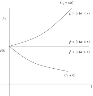
𝑝𝐸= 𝑝𝐸0⋅ exp (𝛽 ⋅ 𝑡) , (23)
where,
𝛽 = 𝑟𝑁− 𝛼, (24)
that is, the difference between the interest rate of
nonex-tracted resources, 𝑟𝑁, and the extraction rate, 𝛼, is a
new parameter called “price increase factor of extracted resources,” PIFE. The price evolution with time of the
extracted resources, given by (23), is shown inFigure 4.
The price of extracted resources evolves with time
accord-ing to the value of PIFE,𝛽. If the extraction rate 𝛼 is equal
t (t0+ ∞) pE pE0 𝛽 > 0, (𝛼 < r) 𝛽 = 0, (𝛼 = r) 𝛽 < 0, (𝛼 > r) (t0+ 0)
Figure 4: Time evolution of the price of extracted resources.
increase factor, PIFE is equal to zero,𝛽 = 0, and the price 𝑝𝐸
remains constant with time. If the extraction rate𝛼 is higher
than𝑟𝑁, the price increase factor, PIFE is negative,𝛽 < 0,
and the price𝑝𝐸decreases with time. If the extraction rate𝛼
is lower than𝑟𝑁, the price increase factor, PIFE is positive,
𝛽 > 0, and the price 𝑝𝐸 increases with time. In case of a
conservative policy of extraction; that is,𝛼 < 0, the price
increase factor, is greater than zero,𝛽 > 0, and the price 𝑝𝐸
increases with time.
5. Mass and Energy-Capital Conservation
Equations of Selling Resources
Assume that nonextracted and extracted energy resources are
in the two reservoirs,𝐶𝑁and𝐶𝐸, ofFigure 5.
The nonextracted resources are in the reservoir𝐶𝑁with
mass𝑀𝑁and interest rate𝑟𝑁. The mass flow rate of extracted
resources from the reservoir𝐶𝑁is𝐺𝐸while the capital flow
rate, relative to the mass flow rate𝐺𝐸, is𝐺𝐾𝐸. The resources
of the reservoir𝐶𝑁are extracted at the price of the extracted
resources,𝑝𝐸, and allocated in the reservoir𝐶𝐸, where𝑀𝐸is
the mass of extracted resources. The resources of the reservoir
𝐶𝐸are sold at the price𝑝𝑆. The mass flow rate of the selling
resources from the reservoir𝐶𝐸is𝐺𝑆while the capital flow
rate, relative to the mass flow rate𝐺𝑆, is𝐺𝐾𝑆.
The mass conservation equation of the extracted
resources in the reservoir𝐶𝐸is
𝑑𝑀𝐸
𝑑𝑡 = 𝐺𝐸− 𝐺𝑆, (25)
while the relative energy-capital conservation equation is 𝑑 𝑑𝑡(𝐾𝐸) = 𝐺𝐾𝑆− 𝐺𝐾𝐸, (26) Nonextracted energy resources Extracted energy resources CN CE MN, rN ME, rE GE(extracted) pE GS(selling) pS GKE(pE) GKS(pS)
Figure 5: Nonextracted and extracted energy resources.
which becomes 𝑑 𝑑𝑡(𝐺𝑆⋅ 𝑝𝑆) = 𝐺𝑆⋅ 𝑝𝑆⋅ 𝑟𝐸− 𝐺𝐸⋅ 𝑝𝐸⋅ 𝑟𝑁, (27) and finally 1 𝑝𝑆 ⋅ 𝑑𝑝𝑆 𝑑𝑡 + 1 𝐺𝑆 ⋅ 𝑑𝐺𝑆 𝑑𝑡 = 𝑟𝐸− 𝐺𝐸⋅ 𝑝𝐸 𝐺𝑆⋅ 𝑝𝑆 ⋅ 𝑟𝑁. (28)
In case of no-accumulation and no-depletion of the
extracted resources,𝐺𝐸 = 𝐺𝑆, the right term of (25) is zero;
that is, the mass𝑀𝐸of extracted resources in the reservoir
𝐶𝐸is constant with time. The mass flow rates of extracted
and selling resources have the same extraction rate𝛼 from
the reservoirs𝐶𝑁and𝐶𝐸; that is,
1 𝐺𝐸 𝑑𝐺𝐸 𝑑𝑡 = 1 𝐺𝑆 𝑑𝐺𝑆 𝑑𝑡 = 𝛼, (29)
which gives, after integration,
𝐺𝐸= 𝐺𝑆= 𝐺𝐸0⋅ exp ⋅ (𝛼 ⋅ 𝑡) = 𝐺𝑆0⋅ exp ⋅ (𝛼 ⋅ 𝑡) , (30)
and the time evolution is similar to that ofFigure 2.
Equation (28) becomes 1 𝑝𝑆 𝑑𝑝𝑆 𝑑𝑡 + 𝛼 = 𝑟𝐸− 𝑝𝐸 𝑝𝑆𝑟𝑁, (31) or 𝑑𝑝𝑆 𝑑𝑡 = 𝑝𝑆(𝑟𝐸− 𝛼) − 𝑝𝐸⋅ 𝑟𝑁. (32)
The substitution of (23) into (32) and the solution of the
relative differential equation give the time evolution of the price of sold resources
𝑝𝑆= 𝑝∗𝑆0 exp(𝛽 ⋅ 𝑡) + [𝑝𝑆0− 𝑝∗𝑆0] exp (𝛽⋅ 𝑡) , (33)
where
𝛽= 𝑟𝐸− 𝛼, (34)
is called the “Price Increase Factor of Selling resources,” PIFS, and
𝑝𝑆0∗ = 𝑟𝑟𝑁⋅ 𝑝𝐸0
𝐸− 𝑟𝑁 =
𝑟𝑁⋅ 𝑝𝐸0
𝛽− 𝛽 , (35)
The price of selling resources, (33), has an extreme
(maximum or minimum) for the time𝑡𝑚given by
𝑡𝑚 =(𝛽 − 𝛽1 )ln[𝛽 ⋅ (𝑝∗ 𝑆0− 𝑝𝑆0) 𝛽 ⋅ 𝑝∗ 𝑆0 ] . (36) The extreme is a maximum if
𝛽(𝛽− 𝛽) (𝑝𝑆0− 𝑝∗𝑆0) < 0, (37)
otherwise it is a minimum.
The time𝑡𝑚of the extreme is zero if𝑝𝑆0is equal to
𝑝∗∗𝑆0 = 𝑝 ∗ 𝑆0(𝛽− 𝛽) 𝛽 = 𝑟𝑁𝑝𝐸0 𝛽 , (38)
which is called “critical initial price extreme of selling resources,” CIPES.
The time𝑡𝑚of the maximum is greater than zero if
𝑝𝑆0> 𝑝∗∗𝑆0 for𝛽> 𝛽 (i.e., 𝑟𝐸> 𝑟𝑁) , (39)
or
𝑝𝑆0< 𝑝∗∗𝑆0 for𝛽< 𝛽 (i.e., 𝑟𝐸< 𝑟𝑁) . (40)
For𝑝𝑆0= 𝑝∗𝑆0the time of the maximum is
𝑡𝑚= +∞, (41)
for𝛽> 𝛽, or
𝑡𝑚= −∞, (42)
for𝛽< 𝛽.
For𝑟𝑁= 𝑟𝐸, that is,𝛽= 𝛽, 𝑝𝑆is given by
𝑝𝑆= (𝑝𝑆0− 𝑝∗∗𝑆0𝛽𝑡) exp (𝛽𝑡) , (43)
where CIPS, that is,𝑝𝑆0∗, is not defined.
The price of selling resources has an extreme for the time
𝑡𝑚given by 𝑡𝑚= (𝑝𝑆0− 𝑝 ∗∗ 𝑆0) 𝑝∗∗ 𝑆0𝛽 . (44)
The extreme is a maximum if𝑝𝑆0∗∗ > 0 and a minimum
if𝑝∗∗𝑆0 < 0. The time 𝑡𝑚of the maximum is zero if the initial
price𝑝𝑆0is
𝑝𝑆0= 𝑝∗∗
𝑆0 =𝑟𝑁𝛽⋅ 𝑝𝐸0. (45)
The possible cases can be classified into six categories:
(i) Category 0—𝑟𝑁= 0;
(ii) Category 1:𝑟𝑁> 𝛼, that is, 𝛽 = PIFE > 0;
(iii) Category 2:𝛼 > 𝑟𝑁, that is,𝛽 = PIFE < 0;
(iv) Category 3:𝛼 = 𝑟𝑁, that is,𝛽 = PIFE = 0;
(v) Category 4:𝑟𝑁= 𝑟𝐸, that is,𝛽= 𝛽 or PIFE = PIFS;
(vi) Category 5:𝑟𝑁< 0. t 0 pS 𝛼 < 0, 𝛽 > 0 (t0+ ∞) (t0+ ∞) (t0+ ∞) 𝛼 = 0, 𝛽 = 0 0 < 𝛼 < rE, 𝛽 < 0 (constant) (t0+ 0) Case 0-A, 𝛼 < rE, 𝛽> 0 Case 0-B, 𝛼 = rE, 𝛽= 0, 𝛽 < 0 Case 0-C, 𝛼 > rE, 𝛽< 0, 𝛽 < 0 Category 0, rN= 0 pS0
Figure 6: Price evolution of selling resources for Category 0.
On their side, each category presents the following possible cases.
Category 0 (𝑟𝑁 = 0). If the interest rate of nonextracted
resources is𝑟𝑁 = 0, (i.e., 𝑝𝑆0∗ = 𝑝∗∗𝑆0 = 0), the price evolution
of selling resources is
𝑝𝑆= 𝑝𝑆0exp(𝛽𝑡) , (46)
where𝛽is the PIF of sold resources.
Figure 6presents the price evolution of selling resources
according to the relation between extraction rate, 𝛼, and
interest rate of extracted resources𝑟𝐸.
Case 0-A (𝛼 < 𝑟𝐸, (i.e.,𝛽> 0)). The price 𝑝𝑆increases with
time at different rates, according to the values of𝛼. The rate
of increase is higher for𝛼 < 0, 𝛽 > 0, intermediate for 𝛼 = 0,
𝛽 = 0, and lower for 𝛼 < 𝑟𝐸,𝛽 < 0.
Case 0-B(𝛼 = 𝑟𝐸, (i.e., 𝛽 = 0, 𝛽 < 0)). The price 𝑝𝑆 is
constant with time at𝑝𝑆0.
Case 0-C(𝛼 > 𝑟𝐸, (i.e.,𝛽 < 0, 𝛽 < 0)). The price 𝑝𝑆 is
decreasing with time towards+0.
In conclusion, for𝑟𝑁 = 0 the criterium to evaluate the
price evolution of selling resources,𝑝𝑆, is𝛽. If𝛽 > 0 the
price𝑝𝑆increases, if𝛽 = 0 the price 𝑝𝑆remains constant,
and if𝛽< 0 the price 𝑝𝑆decreases towards+0.
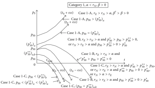
Category 1(𝑟𝑁 > 𝛼, that is, 𝛽 = 𝑃𝐼𝐹𝐸 > 0). The price
evolutions of 𝑝𝑆 are reported in Figure 7 according to the
relation between𝑟𝑁and𝑟𝐸.
Case 1-A(𝑟𝐸 > 𝑟𝑁 > 𝛼, that is, 𝛽 > 𝛽 > 0). The price of
selling resource increases with time if the initial price𝑝𝑆0is
𝑝𝑆0 ≥ 𝑝∗
𝑆0> 𝑝∗∗𝑆0 > 0, that is, equal to or greater than CIPS >
CIPES> 0.
Case 1-B(𝑟𝐸> 𝑟𝑁> 𝛼 and 𝑝𝑆0∗ > 𝑝𝑆0> 𝑝∗∗𝑆0 > 0 or 𝑟𝑁> 𝑟𝐸>
𝛼 and 𝑝𝑆0 > 𝑝𝑆0∗∗ > 0 > 𝑝𝑆0∗). The price of selling resource
Category 1, 𝛼 < rN, 𝛽 > 0 (t0+ ∞) (t0+ ∞) Case 1-A, rE> rN> 𝛼, 𝛽> 𝛽 > 0 Case 1-A, pS0> (p∗S0)a Case 1-A, pS0= (p∗S0)a Case 1-B, rE> rN> 𝛼 and p∗S0> pS0> p∗∗S0> 0, or rN> rE> 𝛼 and pS0> p∗∗S0> 0 > p∗S0 pS pS0 (p∗S0)a pS0 (p∗∗S0)a,b pS0 0 tmax Case 1-B, rE> rN> 𝛼 and p∗S0> pS0> p∗∗S0> 0 (t0− ∞) (t0− ∞) Case 1-C, pS0< (p∗∗S0)a< (p∗S0)a Case 1-C, pS0< (p∗∗S0)b Case 1-C, (pS0= p∗∗S0)a,b Case 1-C, rE> rN> 𝛼 and p∗S0> p∗∗S0> , or rN> rE> 𝛼 and p∗∗S0> pS0> 0 > p∗S0, or rN> 𝛼 > rE Case 1-B, rN> rE> 𝛼 and pS0> p∗∗S0> 0 > p∗S0 pS0 t
Figure 7: Price evolution of selling resources for Category 1.
and then decreases for 𝑟𝐸 > 𝑟𝑁 > 𝛼 if the initial price
𝑝𝑆0has a value comprised between CIPS and CIPES, that is,
𝑝∗
𝑆0 > 𝑝𝑆0 > 𝑝∗∗𝑆0 > 0, or, for 𝑟𝑁 > 𝑟𝐸> 𝛼, if the initial price
𝑝𝑆0is greater than CIPES, that is,𝑝𝑆0> 𝑝∗∗𝑆0 > 0 > 𝑝𝑆0∗.
Case 1-C(𝑟𝐸 > 𝑟𝑁 > 𝛼 and 𝑝∗𝑆0 > 𝑝∗∗𝑆0 > 𝑝𝑆0, or𝑟𝑁 > 𝑟𝐸 >
𝛼 and 𝑝∗∗
𝑆0 > 𝑝𝑆0 > 0 > 𝑝𝑆0∗, or𝑟𝑁 > 𝛼 > 𝑟𝐸). The price of
selling resource decreases with time for𝑟𝐸 > 𝑟𝑁 > 𝛼 if the
initial price𝑝𝑆0is smaller than CIPS and CIPES, that is,𝑝𝑆0∗ >
𝑝∗∗
𝑆0 > 𝑝𝑆0, or, for𝑟𝑁> 𝑟𝐸> 𝛼, if the initial price 𝑝𝑆0is smaller
than CIPES, that is,𝑝𝑆0∗∗> 𝑝𝑆0 > 0 > 𝑝𝑆0∗, or, for𝑟𝑁> 𝛼 > 𝑟𝐸
for every initial price𝑝𝑆0because𝑝𝑆0> 0 > 𝑝𝑆0∗ > 𝑝∗∗𝑆0.
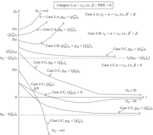
Category 2(𝛼 > 𝑟𝑁, that is,𝛽 = PIFE < 0). The time
evolution is presented inFigure 8according to𝛽 and 𝛽or
the relation between𝑟𝑁and𝑟𝐸.
Case 2-A(𝑟𝐸 > 𝛼 > 𝑟𝑁, that is,𝛽 > 𝛽). The price of selling
resource increases with time if the initial price𝑝𝑆0is𝑝𝑆0 ≥
𝑝∗∗
𝑆0 > 𝑝∗𝑆0, that is, equal to or greater than CIPES > CIPS,
𝑝∗∗
𝑆0 > 𝑝∗𝑆0.
Case 2-B(𝑟𝐸 > 𝛼 > 𝑟𝑁, that is,𝛽 > 𝛽). The price of selling
resource decreases temporarily with time up to𝑡𝑚, given by
(19), and then increases if the initial price, 𝑝𝑆0, has a value
comprised between CIPS and CIPES, that is,𝑝∗𝑆0 > 𝑝𝑆0 >
𝑝𝑆0∗∗> 0.
Case 2-C(𝛼 > 𝑟𝑁, that is,𝛽 < 0). In all other cases the price
of selling resource decreases with time including𝑟𝐸= 𝛼 > 𝑟𝑁,
or𝛼 > 𝑟𝑁> 𝑟𝐸, or𝛼 > 𝑟𝑁> 𝑟𝐸.
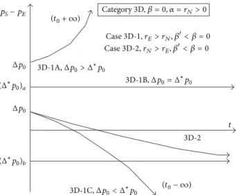
Category 3(𝛼 = 𝑟𝑁, that is,𝛽 = 𝑃𝐼𝐹𝐸 = 0). The price
evolution of selling resources,𝑝𝑆, is dependent on the relation
between𝑟𝑁and𝑟𝐸, as reported inFigure 9.
Case 3-A(𝑟𝐸 > 𝑟𝑁 = 𝛼, that is, 𝛽 > 𝛽 = 0). The price
of selling resource increases with time if the initial price𝑝𝑆0
is 𝑝𝑆0 > 𝑝𝑆0∗∗ = 𝑝𝑆0∗, that is, greater than CIPS = CIPES,
𝑝𝑆0∗∗= 𝑝∗𝑆0.
Case 3-B(𝑟𝐸 > 𝑟𝑁 = 𝛼, that is, 𝛽 > 𝛽 = 0). The price of
selling resource remains constant with time if the initial price
𝑝𝑆0is𝑝𝑆0= 𝑝𝑆0∗∗= 𝑝∗𝑆0, that is, equal to CIPS= CIPES, 𝑝𝑆0∗∗=
𝑝∗
𝑆0.
Case 3-C(𝑟𝐸 > 𝑟𝑁 = 𝛼, that is, 𝛽 > 𝛽 = 0, or 𝑟𝑁 = 𝛼 >
𝑟𝐸, that is,𝛽< 𝛽 = 0). The price of selling resource, for 𝑟𝐸>
𝑟𝑁 = 𝛼, decreases with time if the initial price 𝑝𝑆0is𝑝𝑆0 <
𝑝∗∗
𝑆0 = 𝑝∗𝑆0, that is, smaller than CIPS and CIPES,𝑝∗∗𝑆0 = 𝑝∗𝑆0.
In the other cases the price of the selling resource decreases
with time for every value of𝑝𝑆0.
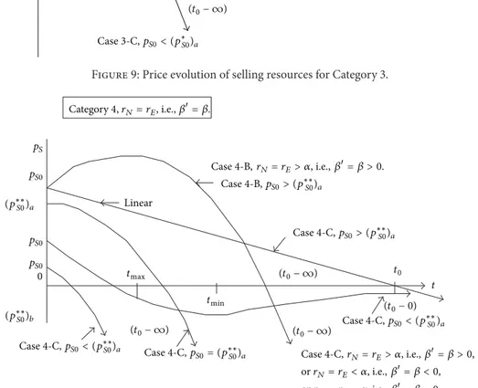
Category 4(𝑟𝑁= 𝑟𝐸, that is,𝛽= 𝛽). The time evolutions are
presented inFigure 10.
Case 4-A(𝑟𝑁= 𝑟𝐸> 𝛼, that is, 𝛽= 𝛽 > 0). The price cannot
increase with time.
Case 4-B(𝑟𝑁 = 𝑟𝐸 > 𝛼, that is, 𝛽 = 𝛽 > 0). The price
of selling resource increases temporarily with time up to𝑡𝑚,
given by (2), and then decreases if the initial price𝑝𝑆0 is
𝑝𝑆0> 𝑝∗∗
𝑆0 > 0, that is, greater than CIPES > 0.
Case 4-C(𝑟𝑁 = 𝑟𝐸 > 𝛼, that is, 𝛽 = 𝛽 > 0, or 𝑟𝑁 = 𝑟𝐸 <
𝛼, that is, 𝛽 = 𝛽 < 0, or 𝑟
𝑁 = 𝑟𝐸 = 𝛼, that is, 𝛽 = 𝛽 = 0).
The price of selling resource decreases with time if the initial
price𝑝𝑆0is𝑝∗∗𝑆0 ≥ 𝑝𝑆0 > 0, that is, equal to or smaller than
CIPES> 0. In all the other cases the price of selling resource
decreases with time for every value of𝑝𝑆0.
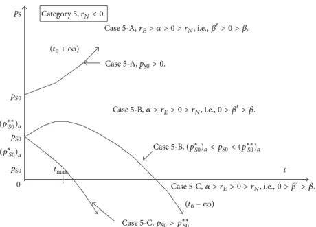
Category 5(𝑟𝑁 < 0). A new category of cases has been
introduced for negative inflation rate, 𝑟𝑁 < 0, which was
registered from March to October, 2009, after the economic crisis of 2008. This new category is interesting because the Hotelling rule forecasts a decrease of the oil price if
t
0
pS
Category 2, 𝛼 > rN, i.e., 𝛽 = PIFE < 0.
(t0+ ∞) pS0 (p∗∗S0)a pS0 (p∗S0)a,b pS0 Case 2-A, pS0> (p∗∗S0)a (p∗∗S0)a (p∗∗S0)a Case 2-A, pS0= Case 2-B, (p∗∗S0)a> ps0>
Case 2-A, rE> 𝛼 > rN, i.e., 𝛽> 𝛽.
Case 2-B, rE> 𝛼 > rN, i.e., 𝛽> 𝛽. Case 2-C, pS0> (p∗S0)b t0(pS0− (p∗S0)b) Case 2-C, pS0= (p∗S0)a Case 2-C, pS0= (p∗S0)b Case 2-C, (p∗S0)c <0 Case 2-C, (p∗S0)d> 0 (t0+ 0) (t0− 0) Case 2-C, pS0< (p∗S0)b (t0− ∞) Case 2-C, pS0< (p∗S0)a Case 2-C 𝛼 > rN, i.e., 𝛽 < 0 pS0− (p∗S0)b pSo− (p∗S0)b
Figure 8: Price evolution of selling resources for Category 2.
the interest rate is assumed to be equal to the inflation rate, that is, negative, while the conclusions of the present approach are different.
The time evolutions are presented inFigure 11.
Case 5-A(𝑟𝐸 > 𝛼 > 0 > 𝑟𝑁, that is,𝛽 > 0 > 𝛽). The price of selling resource increases with time for every value of the
initial price𝑝𝑆0because𝑝𝑆0> 0 > 𝑝𝑆0∗ > 𝑝∗∗𝑆0, since CIPS and
CIPES are negative, or0 > 𝑝∗𝑆0> 𝑝𝑆0∗∗.
Case 5-B(𝛼 > 𝑟𝐸> 0 > 𝑟𝑁, that is,0 > 𝛽> 𝛽). The price of
selling resource increases temporarily with time up to𝑡𝑚and
then decreases if the initial price,𝑝𝑆0, is𝑝∗∗𝑆0 > 𝑝𝑆0> 0 > 𝑝∗𝑆0,
that is, smaller than CIPES> 0 > CIPS.
Case 5-C(𝛼 > 𝑟𝐸> 0 > 𝑟𝑁, that is,0 > 𝛽> 𝛽). The price of
selling resource decreases with time if the initial price,𝑝𝑆0, is
𝑝𝑆0> 𝑝∗∗𝑆0 > 0 > 𝑝∗𝑆0, that is, greater than CIPES> 0 > CIPS.
6. Price Difference between Selling and
Extracted Resources
The difference between selling and extracted resourcesΔ 𝑝 =
(𝑝𝑆− 𝑝𝐸) is defined as Δ 𝑝 = (𝑝𝑆− 𝑝𝐸) = (𝑝𝑆0− 𝑝𝑆0∗) exp (𝛽𝑡) − (𝑝𝐸0− 𝑝∗𝑆0) exp (𝛽𝑡) = (Δ 𝑝0− Δ∗𝑝0) exp (𝛽𝑡) + Δ∗𝑝0exp(𝛽𝑡) , (47) where Δ∗𝑝0= 𝑝𝑆0∗ − 𝑝𝐸0= 𝑝𝐸0(2𝑟𝑁− 𝑟𝐸) (𝑟𝐸− 𝑟𝑁), (48)
is the critical initial price difference, CIPD,Δ∗𝑝0.
The price difference Δ𝑝 has an extreme (maximum or
minimum) for 𝑡𝑚 = 1 (𝛽− 𝛽)ln[ 𝛽 ⋅ (𝑝∗𝑆0− 𝑝𝐸0) 𝛽⋅ (𝑝∗ 𝑆0− 𝑝𝑆0)] = 1 (𝛽− 𝛽)ln[ 𝛽 ⋅ Δ∗𝑝0 𝛽⋅ (Δ∗𝑝 0− Δ 𝑝0)] = (𝛽 − 𝛽1 )ln[𝛽 ⋅ (Δ∗𝑝 0− Δ 𝑝0) 𝛽⋅ Δ∗𝑝 0 ] . (49)
The extreme is a maximum if
𝛽(𝛽− 𝛽) (Δ 𝑝0− Δ∗𝑝0) < 0, (50)
otherwise it is a minimum.
The time𝑡𝑚of the extreme is zero ifΔ𝑝0is equal to
Δ∗∗𝑝0= Δ∗𝑝0[(𝛽
− 𝛽)
t 0 pS pS0 pS0 (p∗S0)a (p∗S0)b
Category 3, 𝛼 = rN, i.e., 𝛽 = PIFE = 0.
Case 3-A, rE> rN= 𝛼, i.e., 𝛽> 0.
Case 3-A, pS0> (p∗S0)a
Case 3-B, rE> rN= 𝛼, i.e., 𝛽> 𝛽 = 0.
Case 3-B, pS0= (p∗S0)a
Case 3-C, rE> rN= 𝛼, i.e. 𝛽> 𝛽 = 0, or rN= 𝛼 > rE, i.e., 𝛽< 𝛽 = 0.
(t0p∗S0)b
Case 3-C (t0+ ∞)
(t0− ∞)
Case 3-C, pS0< (p∗S0)a
Figure 9: Price evolution of selling resources for Category 3.
t 0 pS pS0 pS0 pS0 (p∗∗S0)a (p∗∗S0)b Category 4, rN= rE, i.e., 𝛽= 𝛽. (t0− ∞) (t0− ∞) (t0− ∞) Linear tmax tmin t0 (t0− 0) Case 4-B, rN= rE> 𝛼, i.e., 𝛽= 𝛽 > 0. Case 4-B, pS0> (p∗∗S0)a Case 4-C, pS0> (p∗∗S0)a Case 4-C, pS0< (p∗∗S0)a Case 4-C, pS0< (p∗∗S0)a Case 4-C, p S0= (p∗∗S0)a Case 4-C, rN= rE> 𝛼, i.e., 𝛽= 𝛽 > 0, or rN= rE< 𝛼, i.e., 𝛽= 𝛽 < 0, or rN= rE= 𝛼, i.e., 𝛽= 𝛽 = 0.
Figure 10: Price evolution of selling resources for Category 4.
whereΔ∗∗𝑝0is the critical initial extreme of the initial price
difference, CIEIPD.
The time𝑡𝑚of the extreme is greater than zero if
Δ𝑝0> Δ∗∗𝑝0 for𝛽> 𝛽,
Δ𝑝0< Δ∗∗𝑝
0 for𝛽< 𝛽.
(52)
ForΔ𝑝𝑆0= Δ 𝑝∗𝑆0the time of the extreme is
𝑡𝑚= +∞, (53)
for𝛽> 𝛽, and
𝑡𝑚= −∞, (54)
t 0 pS pS0 pS0 pS0 (p∗∗S0)a (p∗S0)a Category 5, rN< 0.
Case 5-A, rE> 𝛼 > 0 > rN, i.e., 𝛽> 0 > 𝛽.
(t0+ ∞) Case 5-A, pS0> 0. Case 5-B, 𝛼 > rE> 0 > rN, i.e., 0 > 𝛽> 𝛽. tmax Case 5-B, (p∗S0)a< pS0< (p∗∗S0)a Case 5-C, 𝛼 > rE> 0 > rN, i.e., 0 > 𝛽> 𝛽. (t0− ∞) Case 5-C, pS0> p∗∗S0
Figure 11: Price evolution of selling resources for Category 5.
The time𝑡0is 𝑡0= (𝛽1− 𝛽)ln[ Δ ∗𝑝 0 (Δ∗𝑝 0− Δ 𝑝0)] , (55) whenΔ 𝑃 = 0.
The possible cases can be classified in five categories:
Category 0D:𝑟𝑁= 0;
Category 1D:𝑟𝑁> 𝛼, that is, 𝛽 = PIFE > 0;
Category 2D:𝛼 > 𝑟𝑁, that is,𝛽 = PIFE < 0;
Category 3D:𝛼 = 𝑟𝑁, that is,𝛽 = PIFE = 0;
Category 4D:𝑟𝑁= 𝑟𝐸, that is,𝛽= 𝛽 or PIFE = PIFS.
On their side, each category presents the following possible cases.
Category 0D(𝑟𝑁 = 0). The difference between selling and
extracted resources,Δ𝑝, is function of the initial difference
Δ𝑝0 = (𝑝𝑆0− 𝑝𝐸0) and the extraction rate, 𝛼, as compared
to𝑟𝐸. It can be remarked that for𝑟𝑁 = 0 the critical initial
price and differences of sold resources are𝑝𝑆0∗ = 𝑝∗∗𝑆0 = 0,
Δ∗𝑝
0= −𝑝𝐸0, andΔ∗∗𝑝0= −𝑟𝐸𝑝𝐸0/𝛽.
The price difference is then given by
Δ 𝑝 = (𝑝𝑆− 𝑝𝐸) = 𝑝𝑆0exp(𝛽𝑡) − 𝑝𝐸0exp(𝛽𝑡)
= (Δ 𝑝0− Δ∗𝑝0) exp (𝛽𝑡) + Δ∗𝑝0exp(𝛽𝑡) .
(56)
The time𝑡𝑚of the extreme is given by
𝑡𝑚= 1
(𝛽− 𝛽)ln[
𝛽 ⋅ 𝑝𝐸0
𝛽⋅ 𝑝
𝑆0] , (57)
which is obtained for𝑝𝑆0∗ = 0 and the extreme is a maximum
for
𝛽(𝛽− 𝛽) 𝑝𝑆0< 0. (58)
The price difference isΔ 𝑝 = 0 at the time 𝑡0
𝑡0 = 1
(𝛽− 𝛽)ln[
𝑝𝐸0
𝑝𝑆0] . (59)
Four initial conditions are investigated:
(i) if the initial price differenceΔ𝑝0isΔ𝑝0≥ 0 or (𝑝𝑆0≥
𝑝𝐸0);
(ii) if the initial price differenceΔ𝑝0is0 > Δ 𝑝0≥ Δ∗∗𝑝0;
(iii) if the initial price differenceΔ𝑝0isΔ∗∗𝑝0 > Δ 𝑝0 >
Δ∗𝑝0;
(iv) if the initial price differenceΔ𝑝0 isΔ∗𝑝0 = Δ 𝑝0 or
𝑝𝑆0= 𝑝∗𝑆0.
The time evolutions are presented inFigure 12.
Case 0D-A(𝛼 ≤ 0 < 𝑟𝐸, (i.e.,𝛽> 0, 𝛽> 𝛽, (Δ∗∗𝑝0)𝑎< 0))
Case 0D-A1. If the initialΔ𝑝0≥ 0, Δ𝑝 increases exponentially
towards +∞ with a higher rate for 𝛼 < 0, (𝛽 > 0), an
intermediate one for𝛼 = 0, (𝛽 = 0), and a smaller one for
𝑟𝐸> 𝛼 > 0, (𝛽 < 0).
Case 0D-A2. If the initial Δ𝑝0 is 0 > Δ 𝑝0 > Δ∗∗𝑝0 the
evolution is similar to the previous case but nowΔ𝑝 increases
Category 0D, rN= 0. pS− pE (Δ∗∗p0)c pS0 Δp0 0 pS0 0 Δp0 pS0 (Δ∗∗p0)a Δp0 Δ∗p0 0D-A1, 𝛼 < 0, 𝛽 > 0 0D-A1, 𝛼 = 0, 𝛽 = 0 Δp0 (t0+ ∞) (t0+ ∞) Case 0D-A, rE> 𝛼 > 0, 0 > 𝛽 0D-A1, 𝛼 > 0, 0 > 𝛽 0D-B1 0D-B1 0D-C1 tmax tmax (t0+ 0) (t0+ 0) (t0+ 0) t t t 0D-A2, 𝛼 < 0, 𝛽 > 0 (t0+ ∞) 𝛼 = 0, 𝛽 = 0 0D-A2, 0D-A2, 𝛼 > 0, 0 > 𝛽 (t0pS0) (t0pS0) (t0pS0) t0 t0 0D-C2 0D-A3, 𝛼 < 0, 𝛽 > 0 Case 0D-B, 𝛼 = r E, 𝛽= 0, 𝛽 < 0 Case 0D-C, 𝛼 > rE, 0 > 𝛽> 𝛽 tmin 0D-C3 0D-C4 0D-B1 (t0− ∞)
Figure 12: Price difference evolution for Category 0D.
the same pointΔ 𝑝 = 0 at 𝑡0. If the initialΔ𝑝0 = Δ∗∗𝑝0,Δ𝑝
increases exponentially with the minimum at𝑡min = 0.
Case 0D-A3. If the initial Δ𝑝0 is Δ∗∗𝑝0 > Δ 𝑝0 > Δ∗𝑝0
and𝛽 > 0, Δ𝑝 decreases initially to a minimum and then
increases exponentially as in the previous cases.
Case 0D-B(𝛼 = 𝑟𝐸, (i.e.,𝛽= 0 > 𝛽, 𝑝𝑆0∗∗is not defined and
Δ∗∗𝑝
0= −∞ < Δ∗𝑝0< 0))
Case 0D-B1. If the initialΔ𝑝0≥ Δ∗𝑝0,Δ𝑝 tends towards 𝑝𝑆0=
Δ𝑝0− Δ∗𝑝
0as asymptote.
Case 0D-C(𝛼 > 𝑟𝐸, (i.e.,𝛽 < 𝛽 < 0, (Δ∗∗𝑝0)𝑐 > 0 >
(Δ∗𝑝
0)𝑐))
Case 0D-C1. If the initial valueΔ𝑝0 ≥ Δ∗∗𝑝0, the difference Δ𝑝 decreases towards +0, with the maximum at 𝑡 = 0 for
Δ𝑝0= Δ∗∗𝑝0.
Case 0D-C2. If the initial valueΔ∗𝑝0 < Δ 𝑝0 < Δ∗∗𝑝0, the
differenceΔ𝑝 increases up to the time 𝑡maxwhenΔ𝑝 reaches
a maximum value,Δ𝑝max, and then decreases towards+0.
Case 0D-C3. If the initialΔ𝑝0 = Δ∗𝑝0,Δ𝑝 increases towards 0.
Case 0D-C4. If the initial valueΔ𝑝0 = Δ∗𝑝0 < Δ∗∗𝑝0,Δ𝑝
decreases towards−∞ for 𝛽 > 0, tends to 0 for 𝛽 < 0, and
remains constant for𝛽 = 0.
In conclusion, for𝑟𝑁 = 0, the criteria to evaluate the
evolution ofΔ𝑝 are the extraction rate 𝛼 and the initial value
Δ𝑝0. If𝛼 < 𝑟𝐸,Δ𝑝 increases towards +∞ if the initial Δ𝑝0
isΔ𝑝0 > Δ∗𝑝0. If𝛼 = 𝑟𝐸,Δ𝑝 tends towards the asymptotic
value𝑝𝑆0= Δ 𝑝0− Δ∗𝑝0, forΔ𝑝0≥ Δ∗𝑝0. If𝛼 > 𝑟𝐸,Δ𝑝 tends
towards+0 if Δ𝑝0≥ Δ∗𝑝0.
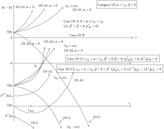
Category 1D(𝑟𝑁 > 𝛼, that is, 𝛽 = 𝑃𝐼𝐹𝐸 > 0). The price
evolution of the difference between selling and extracted
resources,Δ𝑝, is investigated according to the initial value
Δ𝑝0 = (𝑝𝑆0 − 𝑝𝐸0) and the extraction rate 𝛼, as compared
to𝑟𝐸.
Case 1D-A(𝛼 ≤ 0 < 𝑟𝑁 < 𝑟𝐸, (i.e.,𝛽 > 𝛽 > 0, 𝑝∗𝑆0 ≥ 0)).
Three relations between𝑟𝐸and𝑟𝑁can be investigated:
(i)𝑟𝐸> 2𝑟𝑁, that is,(Δ∗𝑝0)𝑎 < (Δ∗∗𝑝0)𝑎 < 0;
(ii)𝑟𝐸= 2𝑟𝑁, that is,(Δ∗𝑝0)𝑎 = (Δ∗∗𝑝0)𝑎 = 0;