Atmospheric deposition, CO
2
, and
change in the land carbon sink
M. Fernández-Martínez
1,2, S. Vicca
3, I. A. Janssens
3, P. Ciais
4, M. Obersteiner
5, M. Bartrons
1,2,
J. Sardans
1,2, A. Verger
1,2, J. G. Canadell
6, F. Chevallier
4, X. Wang
7,8, C. Bernhofer
9, P. S. Curtis
10,
D. Gianelle
11,12, T. Grünwald
9, B. Heinesch
13, A. Ibrom
14, A. Knohl
15, T. Laurila
16, B. E. Law
17,
J. M. Limousin
18, B. Longdoz
19, D. Loustau
20, I. Mammarella
21, G. Matteucci
22,23, R. K. Monson
24,
L. Montagnani
25,26, E. J. Moors
27,28, J. W. Munger
29, D. Papale
30, S. L. Piao
7,31& J. Peñuelas
1,2 Concentrations of atmospheric carbon dioxide (CO2) have continued to increase whereas atmospheric deposition of sulphur and nitrogen has declined in Europe and the USA during recent decades. Using time series of flux observations from 23 forests distributed throughout Europe and the USA, and generalised mixed models, we found that forest-level net ecosystem production and gross primary production have increased by 1% annually from 1995 to 2011. Statistical models indicated that increasing atmospheric CO2 was the most important factor driving the increasing strength of carbon sinks in these forests. We also found that the reduction of sulphur deposition in Europe and the USA lead to higher recovery in ecosystem respiration than in gross primary production, thus limiting the increase of carbon sequestration. By contrast, trends in climate and nitrogen deposition did not significantly contribute to changing carbon fluxes during the studied period. Our findings support the hypothesis of a general CO2-fertilization effect on vegetation growth and suggest that, so far unknown, sulphur deposition plays a significant role in the carbon balance of forests in industrialized regions. Our results show the need to include the effects of changing atmospheric composition, beyond CO2, to assess future dynamics of carbon-climate feedbacks not currently considered in earth system/climate modelling. 1CSIC, Global Ecology Unit, CREAF-CSIC-UAB, Cerdanyola del Vallès, 08193, Barcelona, Catalonia, Spain. 2CREAF,Cerdanyola del Vallès, 08193, Barcelona, Catalonia, Spain. 3Centre of Excellence PLECO (Plant and Vegetation
Ecology), Department of Biology, University of Antwerp, 2610, Wilrijk, Belgium. 4Laboratoire des Sciences du Climat
et de l’Environnement, CEA CNRS UVSQ, 91191, Gif-sur-Yvette, France. 5International Institute for Applied Systems
Analysis, Schlossplatz 1, 2361, Laxenburg, Austria. 6Global Carbon Project, CSIRO Oceans and Atmosphere, Canberra,
ACT 2601, Australia. 7Sino-French Institute of Earth System Sciences, College of Urban and Environmental Sciences,
Peking University, Beijing, 100871, China. 8Laboratoire de Météorologie Dynamique, Université Pierre et Marie
Curie, Paris, 75005, France. 9TU Dresden, Institut für Hydrologie und Meteorologie, LS Meteorologie, Pienner Str. 23,
01737, Tharandt, Germany. 10Department of Evolution, Ecology, and Organismal Biology, The Ohio State University,
Columbus, Ohio, 43210, USA. 11Foxlab Joint CNR-FEM Initiative, Via E. Mach 1, 38010 San Michele all’Adige, Italy. 12Department of Sustainable Agro-Ecosystems and Bioresources, Research and Innovation Center, Fondazione
Edmund Mach, 38010 S, Michele all’ Adige Trento, Italy. 13Department of Biosystem Engineering (BioSE), Gembloux
Agro-Bio Tech, University of Liege, Liège, 4000, Belgium. 14Department of Environmental Engineering, Technical
University of Denmark (DTU), Lyngby, Denmark. 15Bioclimatology, Faculty of Forest Sciences and Forest Ecology,
University of Göttingen, Büsgenweg 2, 37077, Göttingen, Germany. 16Finnish Meteorological Institute, Erik Palménin
aukio 1, FI-00560, Helsinki, Finland. 17Department of Forest Ecosystems & Society, Oregon State University, Corvallis,
OR, 97331, USA. 18Centre d’Ecologie Fonctionelle et Evolutive CEFE, UMR 5175, CNRS, Université de Montpellier,
Université Paul-Valery Montpellier, EPHE, 1919 route de Mende, 34293, Montpellier 5, France. 19UMR Ecologie et
Ecophysiologie Forestières, UMR1137, Inra-Université de Lorraine, Champenoux (F-54280)-Vandoeuvre Les Nancy (F-54500), France. 20INRA, UMR 1391 ISPA, Centre de Bordeaux Aquitaine, Villenave-d’Ornon, France. 21Department
of Physics, University of Helsinki, P.O. Box 48, FIN-00014, Helsinki, Finland. 22IBAF - National Research Council of Italy,
I-00015, Monterotondo (RM), Italy. 23ISAFOM - National Research Council of Italy, I-87036, Rende (CS), Italy. 24School of
Natural Resources and the Environment and Laboratory of Tree Ring Research, University of Arizona, Tucson, Arizona, USA. 25Forest Services, Autonomous Province of Bolzano, Via Brennero 6, 39100, Bolzano, Italy. 26Faculty of Science
and Technology, Free University of Bolzano, Piazza Universit 5, 39100, Bolzano, Italy. 27Alterra Wageningen UR, PO
Box 47, 6700 AA, Wageningen, Netherlands. 28VU University Amsterdam, Boelelaan 1085, Amsterdam, Netherlands. 29School of Engineering and Applied Sciences, Harvard University, Cambridge, MA, 02138, USA. 30DIBAF, University of
Tuscia, 01100, Viterbo, Italy. 31Institute of Tibetan Plateau Research, Chinese Academy of Sciences, Beijing, 100085,
China. Correspondence and requests for materials should be addressed to M.F.-M. (email: [email protected]) Received: 25 January 2017
Accepted: 18 July 2017 Published: xx xx xxxx
Terrestrial ecosystems are key components of the global carbon cycle. Since the 1960s, they have been seques-tering an average of about 30% of the annual anthropogenic CO2 emitted into the atmosphere1. The increase in atmospheric CO2 concentration (hereafter CO2) affects the terrestrial biosphere in multiple ways: warming the climate (radiative effect)2, increasing photosynthesis (CO
2 fertilization), decreasing transpiration by stimulating stomatal closure (leading to increased water-use efficiency) and changing the stoichiometry of carbon, nitrogen and phosphorus (C:N:P) in ecosystem carbon pools3. Although Earth system models simulate rising CO
2 to make a significant contribution to increasing plant productivity and C storage, empirical evidence remains elusive4. This
uncertainty is evidenced by the fact that many studies reporting observations of large-scale increases in produc-tivity (or “greening”) in the Northern Hemisphere have attributed these increases to different contributing mech-anisms. These mechanisms include the CO2-fertilization effect (i.e., more CO2 leads to more photosynthesis), the lengthening of the growing season due to higher winter, spring or autumn temperatures5, nitrogen deposition6,
recovery from acidic deposition7 and afforestation or forest regrowth8. Here, we combine all these potential
driv-ers to reveal the dominant drivdriv-ers of the increase in C fluxes across 23 northern hemisphere forests.
Many experimental studies have shown that productivity increases when ecosystems are exposed to artificially elevated CO29. However, despite being highly valuable, these experiments do not resemble natural conditions because they cannot capture the long-term responses of mature forest ecosystems to gradually increasing CO2 concentrations. In this sense, a CO2-fertilization effect has not yet been firmly established in terrestrial ecosys-tems so far. Positive effects of increasing CO2 on productivity are, in fact, only expected when other factors are not limiting growth (e.g., water and nutrient availability)10. Some studies attributed increased ecosystem water-use
efficiency to the reduction in transpiration resulting from increased CO211, but they have not always been able to link it to enhanced plant growth10, 12.
Detecting a fertilization effect from increasing CO2 in terrestrial ecosystems is difficult because many other factors, that also alter ecosystem productivity trends, are changing concurrently. One of such confounding var-iable is the physical change in climate, which alters ecosystem productivity directly by impacting the ecosys-tem C cycle, and indirectly by increasing nutrient mineralization rates and the length of the growing season. Atmospheric deposition of nitrogenous and sulphurous compounds (N and S deposition) also alter ecosystem processes.
There is strong evidence indicating that N deposition has increased the terrestrial C sink13–16. By acidifying the
soil, sulphur deposition can reduce plant growth and increase leaching of soil nutrients needed by plants17. Some
studies have shown that reduced S deposition is associated with recovery in tree growth through increased net photosynthesis and stomatal conductance18, however, the role of S deposition on forest productivity and C storage
has rarely been explored19. In Europe and North America, air-quality policies to reduce emissions of pollutants
(SO2 and NOx) have proven effective and have decreased acidic deposition (mainly SO42− and NO3−) substan-tially since 198020, 21. The reduction in acidic deposition of both N and S should lead to a slow recovery of forests
to a pre-acid deposition state. On the other hand, decreasing N deposition could also slow down forest growth and C sequestration once previously accumulated soil N is used up and N again becomes a limiting nutrient15, 22.
Here, we test the hypothesis that gross primary production (GPP), ecosystem respiration (Re) and the net C-sink strength (net land-atmosphere CO2 flux) or net ecosystem production (hereafter NEP), have accelerated during the last two decades because of the increased atmospheric CO2 concentrations and temperature, and because of the recovery from high loads of S deposition in Europe and North America. However, decreasing atmospheric deposition of N may have constrained productivity. We expected these deposition reductions to have modulated the biogeochemical effects of rising CO2.
To test our hypothesis, we used long-term eddy-covariance observations of NEP, derived GPP, and Re from 23 temperate and boreal forest sites distributed across Europe and the USA (see Supplementary Fig. S1). For these 23 forests, we also used remotely sensed maximum leaf area index (LAI) as a proxy for canopy development, derived from the AVHRR GIMMS NDVI3g data set23. Data for predictor variables were acquired from: i) gridded
maps for wet N and S deposition for Europe (European Monitoring and Evaluation Programme)24 and the USA
(National Atmospheric Deposition Program)25, and ii) historical climate data from the Climatic Research Unit
(TS v.3.21) for time series of temperature, precipitation26 and the Standardized Precipitation-Evapotranspiration
Index (SPEI) — a measure of meteorological drought27.
Results
Individual trends of NEP, GPP, Re, LAI and predictor variables.
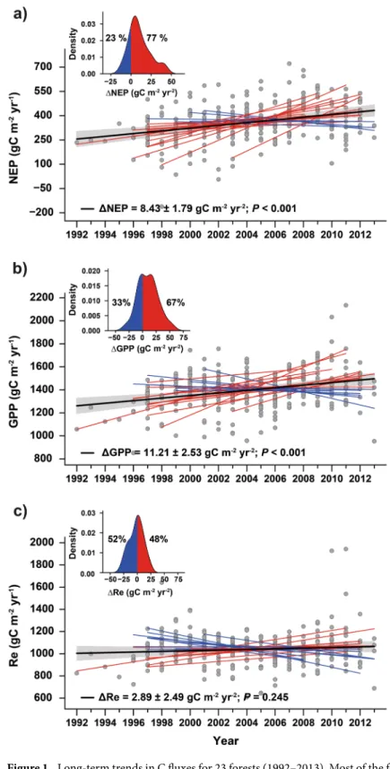
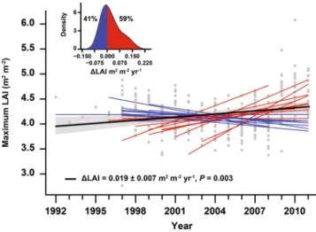
Averaged across the 23 temper-ate and boreal forests, annual NEP and GPP increased (mean ± SE) by 8.4 ± 1.8 and 11.2 ± 2.5 g C m−2 yr−1, respectively, during the studied period (P < 0.001). The increase corresponds to an annual increase of 1.1% in both C fluxes, consistent in magnitude with growth rates reported in previous studies28 and simulated by globalmodels in response to rising CO2 only29. NEP increased over time in 18 of the 23 forests; for 11 of these 18 the increase was statistically significant at P < 0.05 (Fig. 1a inset, Table 1). Bootstrapping analysis show that forests with increasing NEP clearly outnumbered those in which NEP did not increase (P = 0.001; Fig. 1a). Similarly, GPP increased over time in 14 of the 23 forests, with eight forests presenting statistically significant trends at P < 0.05 (Fig. 1b, Table 1). Re of individual forests increased by 2.9 ± 2.5 g C m−2 yr−2, but this signal was not sta-tistically significant (P = 0.25). This led NEP to increase slightly less than GPP, (Fig. 1c and Table 1). Additionally, we found maximum LAI derived from satellite data to exhibit an overall increasing trend (0.019 ± 0.007 m2 m−2 yr−1, P = 0.003) across the 23 forests (Fig. 2). Maximum LAI increased for 14 of the 23 forests, being a statistically significant increase for 5 of these 14 forests.
Across the 23 forests in Europe and USA, CO2 increased on average by 2.0 ± 0.1 ppm yr−1, but neither mean annual temperature (MAT) nor the hydric conditions (SPEI) changed significantly over the same period (Tables S1 and S2, Fig. 3). This apparent climatic stability may partly result from the relatively short time series
Figure 1. Long-term trends in C fluxes for 23 forests (1992–2013). Most of the forests presented increasing trends in (a) NEP and (b) GPP, whereas (c) respiration remained fairly constant. The percentage of forests with increasing NEP was statistically higher (P = 0.001) than the percentage of forests with decreasing NEP, but the percentage of forests where GPP tended to increase was not statistically different (P = 0.28) from those with decreasing GPP. Red and blue lines indicate forests with increasing and decreasing trends, respectively, and black lines indicate the average trends. The shaded area indicates the standard error of the average trend. Grey dots indicate forest-year observations, and all values were adjusted to the same mean to remove forest-specific variability. The inset shows the modelled distribution of the trends using kernel-density estimation, indicating the percentage of forests with increasing and decreasing trends. See Methods for further information on the methodology used to calculate the trends. All data came from eddy-covariance towers.
analysed (10 to 20 years). Conversely, N and especially S deposition exhibited strong and in generally monotonic downward trends from 1995 to 2011 across the 23 forests. On average, N deposition decreased by 1.1% annu-ally (−0.09 ± 0.02 kg N ha−1 yr−2; P < 0.001) and S deposition by 4.6% annually (−0.09 ± 0.01 kg S ha−1 yr−2; P < 0.001) (Tables S1 and S2, Fig. 3).
Spatial variability in individual trends of NEP, GPP, Re and LAI.
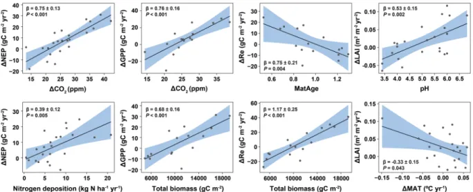
A regression analysis of the indi-vidual trends (see Supplementary Information 1 and Fig. 4) indicates that the annual trends of NEP and GPP were mostly positively correlated with the increasing trend of CO2 (Fig. 4). Forests with larger standing biomass presented more positive trends in GPP and especially Re but not in NEP. Instead, trends of NEP were higher in forests with higher N deposition. Within forests, Re increased with positive trends of MAT, which, conse-quently, reduced trends of NEP. Older forests presented lower or more negative trends of Re than young forests (Supplementary Information 1, Fig. 4). Our analysis did not show significant statistical associations between C flux trends in individual forests and other possible factors (e.g., trends in S deposition, see Supplementary Fig. S2) or forest characteristics, such as mean annual precipitation, soil pH, or leaf type and habit. However, trends in maximum LAI presented a positive association with soil pH and a negative association with trends in MAT (Supplementary Information 1 and Fig. 4).Drivers of trends in C fluxes: temporal contributions and sensitivities.
We used generalized linear mixed models (GLMMs) and model averaging to attribute the temporal trends of NEP, GPP and Re to changes in CO2, N and S deposition rates, MAT, SPEI, LAI and their interactions by calculating the difference between trends predicted by the full model and those maintaining one of the temporal covariates (i.e., anomalies) constant at a time (see Methods for further details). We found that increasing CO2 is the only predictor systematically associ-ated with the observed increase in both NEP and GPP over time (Fig. 5). For each ppm increase in atmospheric CO2 concentration, NEP and GPP increased by 4.81 ± 0.52 and 4.49 ± 0.75 g C m−2 yr−1, respectively (Table 2). Conversely, increasing CO2 had no statistically significant association with increasing Re (Fig. 5) despite the nor-mally close relationship between Re and GPP15. The statistical models also show that the decrease of S depositionduring the period of flux measurements at both European and USA forests (Fig. 3 and Table S2) has also affected the CO2 fluxes in these forests (Fig. 5).
Forest Code Climate Forest Type Age Maturity Age Corrected Mat. Age Initial year Finalyear Y NEP TS Trend P GPP TS Trend P Re TS Trend P LAITS Trend P Brasschaat1 BE-Bra Temp M 80 90 0.89 1997 2011 14 17.5 ± 7.5 0.0773 21.4 ± 13.9 0.0313 9.7 ± 19.8 0.2556 0.000 ± 0.008 0.6329
Castelporziano2 IT-Cpz Temp EB 61 75 0.81 1997 2008 10 2.8 ± 6.9 0.3603 −12.8 ± 16.9 0.7629 −22.1 ± 12.8 0.8145 0.100 ± 0.010 0.0173
Collelongo3 IT-Col Temp DB 118 95 1.24 1997 2012 12 4.1 ± 9.6 0.2686 16.8 ± 11.9 0.1219 8.5 ± 6.4 0.0574 −0.014 ± 0.015 0.8299
Hainich4 DE-Hai Temp DB 275 95 2.89 2000 2012 13 −7.3 ± 4.6 0.9197 −11.2 ± 7.3 0.8502 −6.3 ± 5.9 0.7489 0.047 ± 0.018 0.0466
Harvard5 US-Ha1 Temp DB 81 75 1.07 1992 2011 20 12.6 ± 5.9 0.0372 34.7 ± 5.1 <0.0001 20.2 ± 9.6 0.0075 0.000 ± 0.005 0.6539
Hesse6 FR-Hes Temp DB 43 95 0.45 1996 2010 15 26.4 ± 11.0 0.0374 18.3 ± 15.4 0.1381 0.5 ± 15.3 0.5000 0.017 ± 0.007 0.2737
Howland MT7 US-Ho1 Temp EC 109 90 1.21 1996 2008 13 6.5 ± 2.8 0.0293 −5.8 ± 7.5 0.7489 −16.2 ± 7.2 0.9364 −0.050 ± 0.008 0.9934
Howland F7 US-Ho2 Temp EC 109 90 1.21 1999 2009 11 5.4 ± 4.8 0.1751 7.7 ± 8.2 0.2667 2.6 ± 11.0 0.3202 −0.025 ± 0.011 0.7621 Hyytiala8 FI-Hyy Bor EC 47 90 0.52 1997 2012 16 6.2 ± 2.5 0.0172 14.7 ± 4.0 0.0017 10.4 ± 3.5 0.0051 0.000 ± 0.004 0.5201
Lavarone9 IT-Lav Temp EC 120 90 1.33 2003 2012 10 41.8 ± 10.3 0.0100 37.2 ± 12.8 0.0159 −2.7 ± 5.1 0.7042 0.114 ± 0.022 0.1008
Le Bray10 FR-LBr Temp EC 38 90 0.42 1997 2008 11 7.2 ± 18.8 0.4381 10.8 ± 25.6 0.3777 −18.3 ± 12.6 0.8935 −0.033 ± 0.014 0.8465
Loobos11 NL-Loo Temp EC 88 90 0.98 1997 2012 16 21.5 ± 4.9 0.0009 −6.0 ± 4.2 0.9186 −27.1 ± 5.9 0.9991 −0.017 ± 0.008 0.6559
Metolius12 US-Me2 Temp EC 64 90 0.71 2002 2012 11 13.4 ± 9.8 0.1379 29.0 ± 13.7 0.0806 10.6 ± 13.4 0.2667 0.156 ± 0.028 0.0866
Morgan
Monroe7 US-MMS Temp DB 70 75 0.93 1999 2013 15 −2.6 ± 3.9 0.8619 −1.8 ± 5.5 0.6897 0.7 ± 5.0 0.5000 −0.041 ± 0.009 0.8677
Niwot ridge13 US-NR1 Bor EC 98 90 1.09 1999 2010 12 1.9 ± 2.8 0.4185 −0.1 ± 3.4 0.5000 −1.3 ± 2.3 0.6341 0.060 ± 0.005 0.0166
Park Falls14 US-PFa Temp DB 44 65 0.68 1997 2013 16 9.6 ± 3.7 0.0172 0.1 ± 4.3 0.4820 −12.1 ± 6.2 0.9425 −0.008 ± 0.008 0.5873
Puechabon2 FR-Pue Temp EB 66 75 0.88 2001 2013 13 −10.3 ± 6.6 0.9197 −28.4 ± 13.3 0.9502 −18.5 ± 8.7 0.9880 0.114 ± 0.014 0.0108
Renon15 IT-Ren Bor EC 90 75 1.20 1998 2011 13 37.9 ± 5.3 0.0001 51.9 ± 8.7 0.0006 10.2 ± 6.3 0.0636 0.030 ± 0.007 0.1202
Sodankyla16 FI-Sod Bor EC 75 90 0.83 2000 2012 13 −0.2 ± 1.6 0.5000 −2.8 ± 7.1 0.5243 0.6 ± 6.8 0.4757 0.047 ± 0.005 0.1346
Soroe17 DK-Sor Temp DB 78 95 0.82 1997 2009 13 27.3 ± 4.8 0.0004 22.9 ± 8.4 0.0164 −0.2 ± 8.8 0.5000 −0.017 ± 0.007 0.7336
Tharandt18 DE-Tha Temp EC 117 90 1.30 1997 2013 17 −1.2 ± 3.6 0.6446 16.1 ± 8.3 0.0383 20.4 ± 6.7 0.0178 −0.025 ± 0.014 0.6730
UMBS19 US-UMB Temp DB 79 65 1.22 1999 2012 14 5.4 ± 3.1 0.0080 −3.5 ± 5.4 0.7444 −10.4 ± 4.5 0.9373 0.058 ± 0.005 0.0017
Vielsalm20 BE-Vie Temp M 83 95 0.87 1996 2008 13 17.0 ± 6.9 0.0062 15.1 ± 6.8 0.0120 −0.3 ± 7.2 0.5243 0.2330
Table 1. Summary of the main characteristics of the forests and the trends presented by NEP, GPP, Re, and maximum LAI. Trends were computed using the robust Theil-Sen slope estimator. P indicates a one-tailed P (H1: trend > 0). Corrected maturity age was calculated by dividing the mean stand age by the logging maturity tree age as described by Stokland et al.60 for average productivity classes. Abbreviations: Y, years; TS,
Theil-Sen; Clim for Climate; Temp, temperate; Bor, boreal; for, Forest type; M, mixed; E, evergreen; D, deciduous; B, broadleaved; C, coniferous; EC, eddy covariance. Upperscript numbers indicate reference numbers, see additional References in Supplementary Material.
The reduction in S deposition was associated with a net decrease in NEP (NEP sensitivity: 24.45 ± 15.42 g C m−2 yr−1 for each kg S ha yr−1), likely because of a larger (P = 0.038) increase of Re than GPP as forests recover from past S deposition. The sensitivity of Re and GPP to each kg S ha−1 yr−1 is −74.01 ± 16.02 and −31.24 ± 18.52 g C Figure 2. Trends in forest maximum LAI. Red and blue lines indicate forests with increasing and decreasing trends, respectively, and the thick black line indicates the average trend. The shaded area indicates the standard error of the average trend. Grey dots indicate forest-year observations, and all values were adjusted to the same mean to remove forest-specific variability. The inset shows the modelled distribution of the trends using kernel-density estimation.
Figure 3. Temporal evolution and trends in N and S deposition, mean annual temperature (MAT), SPEI for the 23 forest sites (1995–2011). Trends were calculated using GLMMs with random slopes, with the forest as a random effect and year as a fixed effect. Models also used an ARMA (1,0) autocorrelation structure. Shading indicates the 95% confidence intervals of the means (calculated as 1.96 times the standard error of the mean). See Methods for further details.
m−2 yr−1, respectively. These results imply that the reduction in S deposition reduced the positive effect of CO 2 fertilization on NEP by 21 ± 13%. However, the reduction in N deposition tended to reduce both GPP and Re, but this effect of reduced N deposition was not statistically significant (Fig. 5). The sensitivity of Re and GPP to each kg N ha−1 yr−1 is 15.62 ± 18.65 and 14.41 ± 19.39 g C m−2 yr−1, respectively (see Fig. 5 and Table 2). Using past N and S deposition, i.e. the cumulative totals of the previous 5 years, did not improve our models according to the variance explained, the second-order Akaike Information Criterion (AICc) and the Bayesian Information Criterion (BIC).
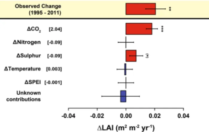
The combined effect of reductions in S and N suggest that the positive effect gained from reduced S depo-sition on GPP and Re was offset by 47 ± 68% and 21 ± 25%, respectively, due to the opposite effect of reduced N deposition. Trends in climate (MAT and SPEI) did not influence trends in CO2 fluxes over the timeframe of this study (1995–2011). Using temperature and SPEI from the warm half of the year (April – September) in our models did not show any greater influence of climate on C flux trends either (see Models 2.2.1–2.2.3 in Supplementary Information). In addition, the increasing LAI was not correlated with the changing C fluxes (Fig. 5, Table 2). Finally, the model used to detect potential causes for the increased LAI showed, again, that rising CO2 and decreased S deposition were the only factors of significant importance for temporal changes across the 23 forests (Fig. 6).
Figure 4. Partial residual plots showing significant relationships found between predictors and C-flux trends in the 23 forests (ΔNEP/Δt, ΔGPP/Δt and ΔRe/Δt) and ΔLAI/Δt. Model summaries can be found in Supplementary Information section 1. Corrected maturity age (MatAge) was calculated by dividing the mean stand age by the logging maturity tree age as described by Stokland et al.60 for average productivity classes. See
Methods for more information on the calculation of the corrected logging maturity age.
Figure 5. Temporal contribution of the predictor variables on NEP, GPP and Re, for the period 1995–2011. Models (see Supplementary Information, section 2.1.1–2.1.3) suggest that increasing CO2 is the main
contributor to the observed increases in NEP and GPP. The difference between the modelled contributions and the observed trends (yellow shaded) has been considered as an unknown contribution to the temporal variation in C fluxes. The temporal variations of the predictors are shown in Fig. 3. Error bars indicate standard errors. Units are ppm for CO2, kg ha−1 yr−1 for S and N deposition, °C for temperature and standard deviation for SPEI. Data for forest C fluxes came from eddy-covariance towers. Error bars indicate standard errors. See Methods for information about the methodology used to calculate the contributions. Significance levels: (*)P < 0.1; *P < 0.05; **P < 0.01; ***P < 0.001.
Discussion
Empirical evidence of CO
2fertilization effect.
Even though our statistical analyses do not directly provecausality, the results provide consistent empirical evidence that support the dominant role of the CO2-fertilization effect in explaining the current positive NEP trends at local and possibly regional scales (Fig. 5). The results sup-port our hypotheses, which were based on the state of the art from earlier studies, refined with respect to other drivers (S deposition), and corroborated by careful attribution of variances with GLMM. The results indicate a relatively strong CO2 fertilization effect given the somewhat short span of CO2 increases in our data set (increas-ing by 13–47 ppm dur(increas-ing the study period, depend(increas-ing on the forest and database, see Table 1 and Supplementary Table S2). This increase is relatively small compared to the increases applied in free-air CO2-enrichment experi-ments (typically 475–600 ppm9, i.e., a step change in CO2 of ~100–200 ppm).
Our results also show a much higher sensitivity of NEP to CO2 of 4.81 ± 0.52 g C m−2 y−1 ppm−1 when com-pared to the sensitivity obtained from CO2-enrichment FACE experiments of 1 g C m−2 y−1 ppm−1, which is a 10% increase in net primary production (assuming an average of 1000 g C m−2 y−1) for a step increase of 100 ppm30, 31.
This discrepancy may be related to the differences between small gradual increases in CO2 seen in the environ-ment versus large stepwise increases in CO2 manipulative experienviron-ments. It has been suggested that the progressive nutrient limitation makes CO2 fertilization be stronger at lower CO2 increases and become saturated at higher levels like the ones in experiments (e.g. 600 ppm)32, 33.
Increasing CO2 can enhance photosynthesis by increasing the rate of carboxylation and reducing losses from photorespiration34. Increasing CO2 might also decrease stomatal conductance, leading to increased water-use
effi-ciency11, 35, but the relationship between increasing water-use efficiency and higher plant growth and net C uptake
in ecosystems is still controversial10, 11. Because tissues with high C:N ratio are more difficult to decompose than
tissues with lower C:N ratio, the increase in litter C:N ratio due to increased CO236 might reduce heterotrophic
respiration37, 38 and, therefore, increase the C-sink strength, at least during a transient period. Elevated CO2,
though, could also stimulate root exudation, thereby increasing the priming effect and reduce soil C stocks39.
NEP P GPP P Re P CO2 (ppm) 4.81 ± 0.52 <0.0001 4.49 ± 0.75 <0.0001 −0.29 ± 0.60 0.3183 Nitrogen (kg ha−1 yr−1) −1.64 ± 15.96 0.4593 14.41 ± 19.39 0.2029 15.62 ± 18.65 0.2044 Sulphur (kg ha−1 yr−1) 24.45 ± 15.42 0.0616 −31.24 ± 18.52 0.0511 −74.01 ± 16.02 <0.0001 Temperature (K) −126.74 ± 408.16 0.4182 −137.36 ± 415.44 0.3716 80.46 ± 592.16 0.4464 SPEI (SD) 13.67 ± 2225.46 0.4976 645.30 ± 6256.23 0.4593 −238.29 ± 3255.54 0.4711 LAI (m2 m−2) −1.80 ± 66.73 0.4893 9.37 ± 76.01 0.4514 28.86 ± 104.40 0.3930 Table 2. NEP, GPP and Re mean sensitivity to predictors for the 23 forests for the period 1995–2011.
Sensitivities (units of change in the response variable for each unit of change in the predictor) were calculated by dividing the temporal contributions of the predictor (Fig. 5) by the trend of the predictors (Figs 2 and 3, Table S2). Nitrogen and sulphur refers to atmospheric deposition, and temperature to mean annual air temperature. Errors were calculated by error propagation63. NEP, GPP and Re units are g C m−2 yr−1. Bold type indicates statistically significant sensitivities.
Figure 6. Temporal contribution of the predictor variables. The model (Supplementary Information, section 2.1.4) suggested that increasing CO2 is the main contributor to the observed increases in LAI. The difference between the modelled contributions and the observed trends has been considered as an unknown contribution to the temporal variation LAI. The temporal variations of the predictors are shown in square brackets. Error bars indicate standard errors. Units are ppm for CO2, kg ha−1 yr−1 for S and N deposition, °C for temperature and standard deviations for SPEI. Error bars indicate standard errors. See Methods for information about the methodology used to calculate the contributions. Significance levels: (*)P < 0.1; *P < 0.05; **P < 0.01; ***P < 0.001.
However, those counteracting mechanisms seem to offset each other in our forests, resulting in no significant change in Re. Nonetheless, despite possible counteracting mechanisms, elevated CO2 seems to be responsible for the increases in terrestrial photosynthesis and C sequestration during the last decades.
Recovery from high loads of acid deposition in Europe and USA.
The negative effect of the reduc-tion in S deposireduc-tion on NEP is the consequence of differences in recovery of the gross fluxes from previously higher rates of acid deposition, i.e. the recovery of Re is stronger than that of GPP (Fig. 5 and Table 2). We postulate that this follows from a chain of processes during recovery from soil acidification. A reduction in S deposition, in our case combined with a reduction in N deposition, typically increases soil pH, which, in turn, increases microbial activity40, thereby increasing heterotrophic respiration and thus nutrient mineralization andavailability41, with implications for both GPP and Re. The potential increase in pH and nutrient availability,
dur-ing a recovery phase after high S deposition, can enhance photosynthesis and tree growth18 in a second step, i.e.
when nutrient availability has considerably increased. Even if pH remains unaltered, reduced acid input reduces aluminium release in soil and, therefore, less damage to roots occur, potentially increasing productivity42. While
higher microbial activity in response to reduced S deposition increases respiration, the associated higher nutri-ent availability can in turn reduce C allocation to root symbionts43 and to free living heterotrophs via exudates,
therefore ultimately reducing heterotrophic respiration44. These two opposing mechanisms may compensate each
other to some degree after some time. The stronger positive response of Re to declining S deposition than of GPP (Fig. 5) suggests a stronger contribution of the increase in microbial respiration, following recovery, than a possi-ble reduction of respiration due to decreased belowground C allocation. Nonetheless, the results obtained here are quite surprising given the relatively small change observed in S deposition that, according to soil models, would have a low impact on soil pH and aluminium release45.
In addition to soil biochemical impacts, reduction in sulphurous pollutants affect optical properties of the atmosphere by reduced secondary aerosol (SOA) formation. S emissions lead to higher aerosol densities, which affect photosynthesis in two opposite ways: by reducing total light inputs, photosynthesis would be reduced, but by increasing the ratio of diffuse over direct radiation, photosynthesis in deeper layers of the canopy would increase46, 47. We speculate, from the overall negative effect of S deposition on GPP, that the disadvantage from
decreasing diffuse light fraction because of reduced S emissions is lower than the positive effect due to the recov-ery from acidification of an ecosystem.
The impacts of N deposition on forest ecosystem C cycling have been widely studied. Reduced heterotrophic respiration is a general response to N deposition, possibly through an enhanced stabilization of soil organic mat-ter, altered plant carbon allocation patterns and shifts in the saprotrophic community48. Nitrogen fertilization
increases aboveground production in young forests, while decreasing autotrophic and heterotrophic respira-tion49, and hence potentially enhancing ecosystem C uptake (or increase C stocks)15, 22. However, in N limited
ecosystems and young stands, low levels of N deposition can increase respiration because of enhanced biomass production and the associated increase in maintenance and growth respiration14, 44. N deposition - where N is a
limiting nutrient - will increase net primary production50 through its effect on photosynthesis51 and possibly by
the above-mentioned increasing C allocation to wood production at the expense of symbionts and exudates43.
Our analysis of spatial variability supported these hypotheses (Supplementary Information, models in section 1 and 2), but our analysis of temporal variability indicated that decreasing N deposition had no statistically signif-icant effect on the trend in NEP, because the small effect of reducing both Re and GPP at the same time (Fig. 5). N deposition rates have been relatively high during several years and the recent decrease (in percentage around a quarter of the decrease in S deposition, see Fig. 3) may have not been large enough to significantly alter C fluxes in forest ecosystems. On the other hand, N is efficiently accumulated and kept in the ecosystem’s internal cycle52,
thereby protecting it from leaching, whereas this is not usually the case for sulphate in acidic soils53.
Small effects of decadal-scale climate change on the carbon balance.
In the 23 forests studied, temperatures and drought did not significantly change and, therefore, could not be responsible for the observed trends in C fluxes. The estimated effect of temperature and drought on CO2 fluxes was clearly small compared to the effects of increasing CO2 and decreasing S deposition. These results suggest that, during the studied period, availability of CO2 and nutrients and stoichiometric changes have exerted a stronger impact on the terrestrial C balance than the changing climate6. Nonetheless, given the small increase in temperatures and droughts duringthe study period, we cannot rule out the possibility that climate change might have larger effects on C fluxes in the future. Larger datasets, including longer time series comprising other geographical regions (i.e., Asia, South America, Africa…) and covering the main biomes of the world, are necessary to correctly answer this question and to better assess the effect of atmospheric deposition on terrestrial C balance.
Changing land carbon sinks.
Multiple drivers are affecting the C budget of terrestrial ecosystems in sev-eral ways. Increasing atmospheric CO2 concentrations have increased the land C sink by enhancing GPP more than ecosystem respiration. The reduction in S deposition rates is severely altering the C balance by enhancing photosynthesis and ecosystem respiration but in a decoupled manner. In addition, the reduction of N deposition rates in developing countries may soon present a significant effect on forest C balances by reducing both photo-synthesis and respiration. However, trends in N and S deposition are divergent depending on the region of the world considered: while S deposition is mainly decreasing in western countries, fossil fuel burning is increasing S deposition rates in Asia54. On the other hand, N deposition is expected to approximately double current levelsby 2050 globally55. Hence, the trends observed for the forests studied here may take place at different regions at
different times in the following decades, unless other nutrient imbalances (e.g., limitation of phosphorus) com-pletely change the response of ecosystems3.
It is far from certain whether terrestrial ecosystems will continue to respond positively to increasing CO2, will saturate, or will eventually reach a tipping point beyond which respiration and the release of greenhouse gases exceed production. Stoichiometric imbalances and the limitation of key nutrients such as nitrogen and phospho-rus3, 6, 56 may already be acting as limiting factors for enhanced C sequestration. Given these observed complex
relationships, partly compensating effects of multiple drivers on the gross C fluxes, GPP and Re, with apparently differing dynamic behaviour, accurate prediction of the future net C sink is complex. It will require biospheric models that include realistic parameterisations of the various biochemical responses of C sequestration processes obtained from real field conditions and experiments. Further, this study shows the need to go beyond climate and CO2 to characterize the strength of the land sink, and the future evolution of the carbon-climate feedback. Biospheric and earth system models will need to develop processes to address the effects of additional atmos-pheric pollutants.
Materials and Methods
Data sets.
Carbon fluxes. We downloaded Level-4 CO2 flux data collected by eddy-covariance towers from the Euroflux (GHG-Europe) and Ameriflux databases. When Level-4 data were not available, we downloaded gap-filled Level-2 data and checked for the homogeneity of the time series. In all cases, time series were either Level-2 or Level-4. Level 4 data are obtained after applying u* filtering, gap-filling and partitioning following Reichstein et al., (2005). Level-2 data are provided by the PIs, half-hourly, not gap-filled or filtered but quality checked by the PIs. This data was then processed using the Eddy covariance gap-filling & flux-partitioning tool from the Max Planck Institute webpage (http://www.bgc-jena.mpg.de/~MDIwork/eddyproc/) to be equivalent to Level-4 data, also following Reichstein et al., (2005). The data used in this study have been harmonized in terms of processing but the fluxes calculation is still heterogeneous because it is performed by the responsible staff of every forest. We also used a global forest database updated in 2013 with data up to 20106 to obtain ancillary data (e.g.,stand age and standing biomass) and for comparing CO2 flux measurements. We selected 23 forests for which at least 10 years of CO2 flux measurements were available. All forests were in the Northern Hemisphere between 39 and 68 °N (see Supplementary Fig. S1), and the years of measurement ranged from 1992 to 2013. These forest sites were selected because they are the longest running flux sites with 10 or more years of data available between 1992 and 2013. The selected forests had no indication of major disturbances or strong management practices which are known to alter C fluxes (in contrast to the typical situation for grasslands or croplands). We also extracted infor-mation for all forests about leaf type and habit (evergreen/deciduous), and the age of the stand at the time of the measurements. Soil pH was extracted from the ancillary data of the forests when possible (17 forests), but when not available, pH was assessed using data from the Harmonized World Soil Database57 (4 forests) and published
literature reviews6 (2 forests).
Remotely sensed LAI data. We calculated the maximum annual LAI for the 23 forests from the GIMMS LAI data set23. The Global Inventory Modeling and Mapping Studies (GIMMS) LAI is derived from Advanced Very High
Resolution Radiometer (AVHRR) satellite time series of the third generation of Normalized Difference Vegetation Index (NDVI3g). It is available at 15-day intervals and 8-km spatial resolution for July 1981 to December 2011. The GIMMS LAI is the only dataset providing time series long enough and with enough temporal resolution to allow the study of trends over the period considered in our study. Furthermore, interannually, GIMMS LAI data were significantly related (P < 0.01) to MODIS LAI (version C5) data for our 23 forests at a resolution of 1 km. The principles used for the generation of the GIMMS LAI data set were based on the use of neural networks that were first trained with data from the overlapping GIMMS NDVI3g and MODIS LAI products. The trained neural network algorithm was then applied using the land-cover class, the latitude and longitude coordinates and the NDVI3g as the input data to generate the full temporal coverage of the GIMMS LAI data set. Further details of the algorithm and quality assessment of GIMMS LAI data set given by Zhu et al.23.
Climate and weather data. We extracted the climatological mean annual temperature and precipitation (MATc, MAPc) for all forests from the WorldClim database, with a spatial resolution of around 1 km at the equator. Because time series of temperature and precipitation data from eddy covariance towers were of insufficient quality (too many missing values) for many of our forests, we opted to use the CRU TS3.21 data set26 from the Climatic
Research Unit to extract temperature and precipitation time series for our forests as weather data. In addition, the SPEI (Standardized Precipitation-Evapotranspiration Index, Vicente-serrano et al.27 from the global SPEI
database (http://sac.csic.es/spei/database.html) was used as a measure of drought intensity. Annual means of temperature (MAT), precipitation (MAP) and SPEI were calculated for each year. We also calculated annual val-ues of MAT, MAP and SPEI for the warm half of the year (April – September) to be tested in the models as done for annual values.
Atmospheric CO2 concentrations. We used atmospheric CO2 concentrations recorded by eddy-covariance towers above the canopies of the forests when available. Annual atmospheric CO2 records, however, sometimes contain implausible values because of gaps along the time series (years with lower CO2 concentrations than the year before, higher than the next year’s or increases much larger than the normal increase of ~2 ppm per year recorded worldwide). We deleted the erroneous annual values and where possible filled the gaps using generalized additive models (GAM), adjusting a smoothing function. When this procedure was not possible, we used atmospheric CO2 concentration data from the Mauna Loa observatory, provided by the Scripps Institution of Oceanography (Scripps CO2 program). Original CO2 records from Mauna Loa and from individual forests were highly corre-lated (P < 0.0001) and their trend was very close to one (1.012 ± 0.005) using a zero intercept mixed model with
random slopes. Therefore, using Mauna Loa’s data instead of original CO2 records from the eddy covariance towers could not influence the outcome of our results.
Deposition data. Annual data for N (NO3− + NH4+) and S (SO4−) wet deposition were extracted from the European Monitoring and Evaluation Programme (EMEP) with a spatial resolution of 0.15 × 0.15° for longitude and latitude, the MSC-W chemical transport model developed to estimate regional atmospheric dispersion and deposition of acidifying and eutrophying compounds of N and S over Europe and the National Atmospheric Deposition Program (NADP) covering the USA with a spatial resolution of 0.027 × 0.027° for longitude and latitude. We used only data for wet deposition because the NADP database did not contain records for dry deposi-tion. Analyses were restricted to Europe and the USA because temporal gridded maps of atmospheric deposition were not available for other regions.
Statistical analyses.
Trends of individual forests. To test whether GPP, Re, NEP, LAI, N and S deposition, MAT and SPEI had changed during the study period, we first analysed the individual (for each forest) annual time series of each of these variables. The trends were extracted using the Theil-Sen slope estimator that minimizes the influence of extreme values (the breakdown point is ca. 29%) when calculating the trends (mblm package58 in Rstatistical software). This analysis has proven to be robust against temporal autocorrelation, non-normality and heteroscedasticity and produces results very similar to those of ordinary least squares regressions when errors are normally distributed and no outliers are present59, 60. Kernel densities were estimated to illustrate the proportions
of forests with increasing and decreasing trends. Bootstrapping was used to statistically test whether the distri-bution of positive and negative trends across the forests was significantly different than the distridistri-bution of trends we would find by chance. We then tested the average trends (over all studied forests) in the studied variables using mixed models with random slopes (e.g., NEP ~ year) where the forest was the random factor (affecting the slopes of the year, therefore the trend). These mixed models also accounted for temporal autocorrelation using an autoregressive moving average (ARMA) (p = 1, q = 0) correlation structure. The average trends shown in the results section, and their significance, were calculated using the mixed effects models explained above.
To account for the spatial variability among forests (N = 23) in the trends of NEP, GPP, Re and LAI we used weighted linear models (adjusted by ordinary least squares and weighting for the number of observations for each forest) and stepwise forward model selection. The predictor variables we tested were climate (MATc and MAPc), mean S and N annual deposition rates, stand age, leaf type and habit, soil pH, the observed trends in LAI, S and N deposition, MAT, SPEI and the increase in CO2 since the beginning of the C-flux measurements. To further test that the observed trends in C fluxes were dependent on the age of the stand, we calculated a surrogate of the state of maturity of the forests by dividing the mean stand age by the logging maturity tree age as described by Stokland et al.60 for average productivity classes and included this variable as a predictor in the model. We also
included the first-order interaction between pH and trends in N and S to test whether the effect of deposition depended on pH and vice-versa. We checked for multicolinearity overseeing the variance inflation factor. The variance explained by each variable within these models was assessed using the proportional marginal variance decomposition (PMVD) metric from the relaimpo R package61.
Temporal contributions and sensitivities of changes in C fluxes. The temporal contribution of each variable to the observed trends in GPP, Re, NEP and LAI was assessed using Generalised Linear Mixed Models (GLMMs) and model averaging (multi-model inference)62. This technique (GLMMs) allows disentangling the effect of
one single predictor, while taking into account the variance shared (or correlation) with the other predictors. Model averaging is a statistical technique based on multi-model inference that calculates an average model with the estimates of the models that best fit the data while weighting their importance using the difference of the second-order Akaike Information Criterion (AICc) between each model and the model with lowest AICc. Using the forest as the random effect and an ARMA (p = 1, q = 0) autocorrelation structure, we fitted the saturated models as: response (annual anomalies) ~ (mean S deposition + S anomalies + CO2) + (mean N deposition + N anomalies + CO2) + (MATc + MAT anomalies + CO2) + (MAPc + SPEI + CO2) + mean S deposition x mean N deposition + MATc x climatic MAPc + CO2 x mean stand age, where variables between brackets where those for which we tested for first order interactions. Anomalies were calculated as the difference between the average value (e.g., MATc) and the annual value of a given year (i.e., MATan = MATc + MAT). When including the interactions between the climatic annual mean and the anomalies (MATc x MATan), we are including a changing effect of increasing or decreasing the anomalies depending on the mean for the forest (e.g., increasing temperature may have a positive effect in cold climates but a negative effect in warmer climates). In C flux models, we also included the anomalies of maximum LAI as a covariate. In our case, LAI can be interpreted as a surrogate for forest man-agement, which implies that the reported effects of increasing CO2 concentrations are disconnected from any changes in forest structure (LAI or crown cover closure). Additionally, we fitted the saturated models using past N and S deposition, i.e. the cumulative totals of the previous 5 years, to test whether cumulative atmospheric deposition could improve prediction of interannual variability of C flux trends.
Using the model-averaging method [MuMIn R package] we fitted the saturated models for GPP, Re, NEP and LAI to construct an average model from the best models nested into the saturated models. 758246 models were calculated for each C flux and 379055 models for LAI. Average models were calculated using those models differing by less than four AICc units (in comparison with the best model) and fitted using restricted maximum likelihood. When calculating the model average estimates of the variables, estimates were replaced with 0 for models in which the explanatory variable was not included. Model residuals met the assumptions of normality, homocedasticity and linearity in all analyses.
We then used the average models to predict the change of the response variables during the study period (1995–2011). With the average models, we first calculated the observed trend (slope estimate ± standard error
of the slope estimate) in our data using GLMMs with random slopes and temporal autocorrelation structure (ARMA, p = 1, q = 0). We then calculated the trend predicted by the average model and the trends predicted by the same model but maintaining the predictors constant one at a time (e.g., S deposition anomalies are held constant, using the median values per forest, while all other predictors change according to the observations). The difference between the predictions for the whole model and when one variable was controlled was the con-tribution of that predictor variable to the change in the response variable. The difference between all individual contributions and the observed trend were considered to be unknown contributions. Finally, we calculated the average NEP, GPP and Re sensitivities to predictor changes dividing the temporal contributions by the trends of the predictor variables. All errors were calculated using the error-propagation method.
References
1. Le Quéré, C. et al. Global Carbon Budget 2015. Earth Syst. Sci. Data 7, 349–396 (2015).
2. Alexander, L. et al. Climate Change 2013: The Physical Science Basis - Summary for Policymakers. Fifth Assessment Report. At: http:// www.climatechange2013.org/. (Intergovernmental Panel on Climate Change, 2013).
3. Peñuelas, J. et al. Human-induced nitrogen-phosphorus imbalances alter natural and managed ecosystems across the globe. Nat.
Commun. 4, 2934 (2013).
4. Ciais, P. et al. 2013: Carbon and Other Biogeochemical Cycles. Clim. Chang. 2013 Phys. Sci. Basis. Contrib. Work. Gr. I to Fifth Assess.
Rep. Intergov. Panel Clim. Chang. 465–570 (2013). doi:10.1017/CBO9781107415324.015
5. Linderholm, H. W. Growing season changes in the last century. Agric. For. Meteorol. 137, 1–14 (2006).
6. Fernández-Martínez, M. et al. Nutrient availability as the key regulator of global forest carbon balance. Nat. Clim. Chang. 4, 471–476 (2014).
7. Büntgen, U. et al. Placing unprecedented recent fir growth in a European-wide and Holocene-long context. Front. Ecol. Environ. 12, 100–106 (2013).
8. Pan, Y. et al. A large and persistent carbon sink in the world’s forests. Science 333, 988–93 (2011).
9. Ainsworth, E. A. & Long, S. P. What have we learned from 15 years of free-air CO2 enrichment (FACE)? A meta-analytic review of the responses of photosynthesis, canopy properties and plant production to rising CO2. New Phytol. 165, 351–71 (2005). 10. Peñuelas, J., Canadell, J. G. & Ogaya, R. Increased water-use efficiency during the 20th century did not translate into enhanced tree
growth. Glob. Ecol. Biogeogr. 20, 597–608 (2011).
11. Keenan, T. F. et al. Increase in forest water-use efficiency as atmospheric carbon dioxide concentrations rise. Nature 499, 324–327 (2013).
12. van der Sleen, P. et al. No growth stimulation of tropical trees by 150 years of CO2 fertilization but water-use efficiency increased.
Nat. Geosci. 8, 24–28 (2014).
13. Magnani, F. NEP and Nitrogen deposition. Nature 1–3, doi:10.1038/nature05847 (2002).
14. de Vries, W., Du, E. & Butterbach-Bahl, K. Short and long-term impacts of nitrogen deposition on carbon sequestration by forest ecosystems. Curr. Opin. Environ. Sustain. 9–10, 90–104 (2014).
15. Fernández-Martínez, M. et al. Spatial variability and controls over biomass stocks, carbon fluxes and resource-use efficiencies in forest ecosystems. Trees, Struct. Funct. 28, 597–611 (2014).
16. Fleischer, K. et al. The contribution of nitrogen deposition to the photosynthetic capacity of forests. Global Biogeochem. Cycles 27, 187–199 (2013).
17. Likens, G. E., Driscoll, C. T. & Buso, D. C. Long-Term Effects of Acid Rain: Response and Recovery of a Forest Ecosystem. Science
272, 244–246 (1996).
18. Thomas, R. B., Spal, S. E., Smith, K. R. & Nippert, J. B. Evidence of recovery of Juniperus virginiana trees from sulfur pollution after the Clean Air Act. Proc. Natl. Acad. Sci. USA 110, 15319–24 (2013).
19. Oulehle, F. et al. Major changes in forest carbon and nitrogen cycling caused by declining sulphur deposition. Glob. Chang. Biol. 17, 3115–3129 (2011).
20. Menz, F. C. & Seip, H. M. Acid rain in Europe and the United States: an update. Environ. Sci. Policy 7, 253–265 (2004).
21. Lajtha, K. & Jones, J. Trends in cation, nitrogen, sulfate and hydrogen ion concentrations in precipitation in the United States and Europe from 1978 to 2010: a new look at an old problem. Biogeochemistry 116, 303–334 (2013).
22. De Vries, W. et al. The impact of nitrogen deposition on carbon sequestration by European forests and heathlands. For. Ecol. Manage.
258, 1814–1823 (2009).
23. Zhu, Z. et al. Global Data Sets of Vegetation Leaf Area Index (LAI)3g and Fraction of Photosynthetically Active Radiation (FPAR)3g Derived from Global Inventory Modeling and Mapping Studies (GIMMS) Normalized Difference Vegetation Index (NDVI3g) for the Period 1981 to 2. Remote Sens. 5, 927–948 (2013).
24. European Monitoring and Evaluation Programme. EMEP MSC-W modelled air concentrations and depositions. EMEP MSC-W
modelled air concentrations and depositions. At: http://www.emep.int/mscw/index_mscw.html (2013).
25. National Atmospheric Deposition Program. Annual NTN Maps by Year. National Atmospheric Deposition Program (NRSP-3). At:
http://nadp.sws.uiuc.edu/ntn/annualmapsByYear.aspx (2013).
26. Harris, I., Jones, P. D. D., Osborn, T. J. J. & Lister, D. H. H. Updated high-resolution grids of monthly climatic observations - the CRU TS3.10 Dataset. Int. J. Climatol. 34, online, update (2013).
27. Vicente-serrano, S. M., Beguería, S. & López-Moreno, J. I. A Multiscalar Drought Index Sensitive to Global Warming: The Standardized Precipitation Evapotranspiration Index. J. Clim. 23, 1696–1718 (2010).
28. Canadell, J. G. et al. Contributions to accelerating atmospheric CO2 growth from economic activity, carbon intensity, and efficiency of natural sinks. Proc. Natl. Acad. Sci. USA 104, 18866–70 (2007).
29. Sitch, S. et al. Trends and drivers of regional sources and sinks of carbon dioxide over the past two decades. Biogeosciences 12, 653–679 (2015).
30. Norby, R. J., Warren, J. M., Iversen, C. M., Medlyn, B. E. & McMurtrie, R. E. CO2 enhancement of forest productivity constrained by limited nitrogen availability. Proc. Natl. Acad. Sci. USA 107, 19368–73 (2010).
31. Smith, K. et al. Large divergence of satellite and Earth system model estimates of global terrestrial CO2 fertilization. Nat. Clim.
Chang. 6, 306–310 (2015).
32. Körner, C. Biosphere responses to CO2 enrichment. Ecol. Appl. 10, 1590–1619 (2000).
33. Norby, R. J. et al. Forest response to elevated CO2 is conserved across a broad range of productivity. Proc. Natl. Acad. Sci. USA 102, 18052–18056 (2005).
34. Aber, J. et al. Forest Processes and Global Environmental Change: Predicting the Effects of Individual and Multiple Stressors.
Bioscience 51, 735 (2001).
35. Prentice, I. C., Heimann, M. & Sitch, S. The carbon balance of the terrestrial biosphere: Ecosystem models and Atmospheric observations. Ecol. Appl. 10, 1553–1573 (2000).
36. Sardans, J., Rivas-Ubach, A. & Peñuelas, J. The C:N:P stoichiometry of organisms and ecosystems in a changing world: A review and perspectives. Perspect. Plant Ecol. Evol. Syst. 14, 33–47 (2012).
37. Hu, S., Chapin, F. S., Firestone, M. K., Field, C. B. & Chiariello, N. R. Nitrogen limitation of microbial decomposition in a grassland under elevated CO2. Nature 409, 188–91 (2001).
38. Norby, R. J., Cotrufo, M. F., Ineson, P., O’Neill, E. G. & Canadell, J. G. Elevated CO2, litter chemistry, and decomposition: a synthesis.
Oecologia 127, 153–65 (2001).
39. Bengtson, P., Barker, J. & Grayston, S. J. Evidence of a strong coupling between root exudation, C and N availability, and stimulated SOM decomposition caused by rhizosphere priming effects. Ecol. Evol. 2, 1843–52 (2012).
40. Andersson, S. & Nilsson, S. I. Influence of pH and temperature on microbial activity, substrate availability of soil-solution bacteria and leaching of dissolved organic carbon in a mor humus. Soil Biol. Biochem. 33, 1181–1191 (2001).
41. Truog, E. Soil Reaction Influence on Availability of Plant Nutrients1. Soil Sci. Soc. Am. J. 11, 305 (1946).
42. Gundersen, P. & Rasmussen, L. in Reviews of Environmental Contamination and Toxicology (Springer, 1990). doi:10.1177/0192513X12437708
43. Vicca, S. et al. Fertile forests produce biomass more efficiently. Ecol. Lett. 15, 520–6 (2012).
44. Janssens, Ia. et al. Reduction of forest soil respiration in response to nitrogen deposition. Nat. Geosci. 3, 315–322 (2010).
45. De Vries, W., Hettelingh, J.-P. & Posch, M. Critical Loads and Dynamic Risk Assessments: Nitrogen, Acidity and Metals in Terrestrial
and Aquatic Ecosystems, Environmental Pollution Volume 25. (Springer, 2015).
46. Mercado, L. M. et al. Impact of changes in diffuse radiation on the global land carbon sink. Nature 458, 1014–1017 (2009). 47. Ibrom, A. et al. A comparative analysis of simulated and observed photosynthetic CO2 uptake in two coniferous forest canopies. Tree
Physiol. 26, 845–864 (2006).
48. Piao, S. et al. Forest annual carbon cost: a global-scale analysis of autotrophic respiration. Ecology 91, 652–661 (2010).
49. Olsson, P., Linder, S., Giesler, R. & Högberg, P. Fertilization of boreal forest reduces both autotrophic and heterotrophic soil respiration. Glob. Chang. Biol. 11, 1745–1753 (2005).
50. Luyssaert, S. et al. The European carbon balance. Part 3: forests. Glob. Chang. Biol. 16, 1429–1450 (2010).
51. Field, C., Merino, J. & Mooney, Ha. Compromises between water-use efficiency and nitrogen-use efficiency in five species of California evergreens. Oecologia 60, 384–389 (1983).
52. Wang, L. et al. Interactions between leaf nitrogen status and longevity in relation to N cycling in three contrasting European forest canopies. Biogeosciences 10, 999–1011 (2013).
53. Lefroy, R. D. B., Santoso, D. & Blair, G. J. Fate of applied phosphate and sulfate in weathered acid soils under leaching conditions.
Aust. J. Soil Res. 33, 135–151 (1995).
54. Kuribayashi, M. et al. Long-term trends of sulfur deposition in East Asia during 1981-2005. Atmos. Environ. 59, 461–475 (2012). 55. Galloway, J. N. et al. Nitrogen Cycles: Past, Present, and Future. Biogeochemistry 70, 153–226 (2004).
56. Fernández-Martínez, M., Vicca, S., Janssens, I. A., Campioli, M. & Peñuelas, J. Nutrient availability and climate as the main determinants of the ratio of biomass to NPP in woody and non-woody forest compartments. Trees, Struct. Funct. 30, 775–783 (2016).
57. Nachtergaele, F. & Velthuizen, H. Van. Harmonized World Soil Database. … World Congr. Soil … 38. At: http://www.fao.org/ uploads/media/Harm-World-Soil-DBv7cv_1.pdf (2010).
58. Lukasz Komsta. mblm: Median-Based Linear Models. At: http://cran.r-project.org/package=mblm (2012).
59. Ohlson, J. A. & Kim, S. Linear valuation without OLS: the Theil-Sen estimation approach. Review of Accounting Studies 20, (2015). 60. Stokland, J. N. et al. Forest biodiversity indicators in the Nordic Countries. Status based on national forest inventories. Tema Nord
2003, 514 (2003).
61. Grömping, U. Relative importance for linear regression in R: the package relaimpo. J. Stat. Softw. 17, 1–27 (2006).
62. Burnham, K. P. & Anderson, D. R. Model Selection and Multimodel Inference: A Practical Information-Theoretic Approach. (Springer, 2004).
63. Ku, H. H. Notes on the use of propagation of error formulas. J. Res. Natl. Bur. Stand. Sect. C Eng. Instrum. 70C, 263–273 (1966).
Acknowledgements
This research was supported by the European Research Council Synergy grant ERC-2013-SyG 610028-IMBALANCE-P, the Spanish Government grant CGL2013–48074-P and the Catalan Government projects SGR 2014–274 and FI-2013. S.V. is a postdoctoral research associate of the Fund for Scientific Research – Flanders. A.V. is the recipient of a Juan de la Cierva fellowship from the Spanish Ministry of Science and Innovation. We thank all site investigators, their funding agencies and the regional flux networks (AmeriFlux, EuroFlux, CarboEuropeIP), and the Fluxnet project, whose support was essential for obtaining the measurements. We appreciate the financial support of the GHG-Europe project. The authors gratefully acknowledge the National Atmospheric Deposition Program (NADP) and the European Monitoring and Evaluation Programme (EMEP) for providing data on N and S deposition in the USA and Europe, respectively. Thanks go to NOAA, Earth System Research Laboratory and Global Monitoring Division, and to the Scripps Institution of Oceanography (Scripps CO2 program) for providing the data for atmospheric CO2 concentrations from Point Barrow and Mauna Loa, respectively. J.G.C. thanks the support of the Australian Climate Change Science Programme. We also want to thank the anonymous reviewers of the manuscript for their comments and suggestions that helped us to improve the quality of the manuscript.
Author Contributions
M.F.-M., S.V., I.A.J. and J.P. conceived, analysed and wrote the paper. A.V., F.C., X.W., C.B., P.S.C., D.G., T.G., B.H., A.I., A.K., T.L., B.L., J.M.L., B.L., D.L., I.M., G.M., R.M., L.M., E.J.M., J.W.M., D.P. and S.P. provided the data. P.C., M.O., M.B., J.S. and J.C. contributed substantially to the writing and discussion of the paper.
Additional Information
Supplementary information accompanies this paper at doi:10.1038/s41598-017-08755-8
Competing Interests: The authors declare that they have no competing interests.
Publisher's note: Springer Nature remains neutral with regard to jurisdictional claims in published maps and institutional affiliations.
Open Access This article is licensed under a Creative Commons Attribution 4.0 International License, which permits use, sharing, adaptation, distribution and reproduction in any medium or format, as long as you give appropriate credit to the original author(s) and the source, provide a link to the Cre-ative Commons license, and indicate if changes were made. The images or other third party material in this article are included in the article’s Creative Commons license, unless indicated otherwise in a credit line to the material. If material is not included in the article’s Creative Commons license and your intended use is not per-mitted by statutory regulation or exceeds the perper-mitted use, you will need to obtain permission directly from the copyright holder. To view a copy of this license, visit http://creativecommons.org/licenses/by/4.0/.