Whole ship energy optimization: the case study of a chemical tanker

(1)

ALMA MATER STUDIORUM - UNIVERSITÀ DI BOLOGNA

SCUOLA DI INGEGNERIA E ARCHITETTURA

Dipartimento di Ingegneria Industriale

CORSO DI LAUREA IN INGEGNERIA MECCANICA

TESI DI LAUREA

in

Sistemi Energetici Avanzati e Cogenerazione

Whole Ship Energy Optimization: the Case Study of a

Chemical Tanker

Candidato: RELATORE:

Michele Saccani Chiar.mo Prof. Michele Bianchi

CORRELATORE: Ing. Lisa Branchini

Anno Accademico 2012/2013 Sessione II

(2)

(3)

Abstract -‐ Italiano

La presente dissertazione investiga la possibilità di ottimizzare l’uso di energia a bordo di una nave per trasporto di prodotti chimici e petrolchimici. Il software sviluppato per questo studio può essere adattato a qualsiasi tipo di nave. Tale foglio di calcolo fornisce la metodologia per stimare vantaggi e miglioramenti energetici, con accuratezza direttamente proporzionale ai dati disponibili sulla configurazione del sistema energetico e sui dispositivi installati a bordo. Lo studio si basa su differenti fasi che permettono la semplificazione del lavoro; nell’introduzione sono indicati i dati necessari per svolgere un’accurata analisi ed è presentata la metodologia adottata.

Inizialmente è fornita una spiegazione sul layout dell’impianto, sulle sue caratteristiche e sui principali dispositivi installati a bordo. Vengono dunque trattati separatamente i principali carichi, meccanico, elettrico e termico. In seguito si procede con una selezione delle principali fasi operative della nave: è seguito tale approccio in modo da comprendere meglio la ripartizione della richiesta di potenza a bordo della nave e il suo sfruttamento.

Successivamente è svolto un controllo sul dimensionamento del sistema elettrico: ciò aiuta a comprendere se la potenza stimata dai progettisti sia assimilabile a quella effettivamente richiesta sulla nave.

Si ottengono in seguito curve di carico meccanico, elettrico e termico in funzione del tempo per tutte le fasi operative considerate: tramite l’uso del software Visual Basic Application (VBA) vengono creati i profili di carico che possono essere gestiti nella successiva fase di ottimizzazione. L’ottimizzazione rappresenta il cuore di questo studio; i profili di potenza ottenuti dalla precedente fase sono gestiti in modo da conseguire un sistema che sia in grado di fornire potenza alla nave nel miglior modo possibile da un punto di vista energetico. Il sistema energetico della nave è modellato e ottimizzato mantenendo lo status quo dei dispositivi di bordo, per i quali sono considerate le configurazioni di “Load following”, “two shifts” e “minimal”.

Una successiva investigazione riguarda l’installazione a bordo di un sistema di accumulo di energia termica, così da migliorare lo sfruttamento dell’energia disponibile.

Infine, nella conclusione, sono messi a confronto i reali consumi della nave con i risultati ottenuti con e senza l’introduzione del sistema di accumulo termico. Attraverso la configurazione “minimal” è possibile risparmiare circa l’1,49% dell’energia totale consumata durante un anno di attività; tale risparmio è completamente gratuito poiché può essere raggiunto seguendo alcune semplici regole nella gestione dell’energia a bordo. L’introduzione di un sistema di accumulo termico incrementa il risparmio totale fino al 4,67% con un serbatoio in grado di accumulare 110000 kWh di energia termica; tuttavia, in questo caso, è necessario sostenere il costo di installazione del serbatoio. Vengono quindi dibattuti aspetti economici e ambientali in modo da spiegare e rendere chiari i vantaggi che si possono ottenere con l’applicazione di questo studio, in termini di denaro e riduzione di emissioni in atmosfera.

(6)

Abstract

This dissertation investigates the possibility to optimize the energy use on a chemical tanker. The software created for this study can be adapted to all the ships. This tool provides the methodology to estimate energy advantages and improvements, with accuracy directly proportional to the availability of data on the energy system configuration and on the devices installed on board.

The study is based on different steps that allow the simplification of the work; in the introduction, necessary available data and the adopted methodology are presented.

At first, the plant is introduced through a diagram and by explanation of its main characteristics and components. After that, mechanical, electrical and thermal loads are considered separately, and different operational phases are selected among the working time of the chemical tanker; this approach is made in order to understand better the request of power and its exploitation.

Afterwards, a check on the sizing of the electrical system on board is made: this allows comprehending if the power estimated by the designers is similar to the effective one exploited on the ship.

Later on, curves of mechanical, electrical and thermal power as a function of time for all the operational phases are obtained; power profiles that can be managed during the optimization stage are achieved through the use of the software Visual Basic Application (VBA).

The optimization is the core of the study; power profiles got by the previous stage are managed in order to obtain a system that can provide power to the chemical tanker in the best way from the energy point of view. The energy system of the ship is modelled and optimized, maintaining the status quo of the devices. “Load following”, “two shifts” and “minimal” configurations are put into account in this analysis.

A further investigation is made considering the possibility to install a thermal energy storage system on board, in order to improve the energy configuration and exploitation.

Finally, conclusions are made. Real tanker’s consumption and results obtained with and without the addition of a thermal energy storage system are compared. Through the “minimal” configuration is possible to save about 1,49% of the total energy consumed during one operational year; this saving is completely “free” because it can be achieved only by following some simple rules in energy management. The addition of the energy storage increases the total saving up to 4,67% with a tank capacity of about 110000 kWh; however, in this case the tank installation cost is expected. Economical and environmental discussions are made in order to clarify and explain the advantages that can be achieved in terms of money and emissions.

(7)

Introduction

i.1 Background

i.1.1 International Shipping

Today, shipping is one of the largest drives of world’s globalised economy, as it contributes to more than 80% of global world trade by volume, and 70% by value. The evolution of global trade in the last decades suggests a big increase even after the step back caused by the economic crisis in 2008, and this growing trend is very likely to continue in the future, fostered by the growth in non-OECD countries (Organisation for Economic Cooperation and Development) [17].

As a result of this trend, merchant shipping has been growing steadily over the past years, hand in hand with world trade. In the period between 1999 and 2004 merchant shipping increased its economic turnover by a striking average of 22% per year [17]. This growth, together with the rising global economy, is explained by phenomena like containerisation, increased economy of scale, and advances in marine engineering [17]. Under these conditions, the cost of freight is not a major concern anymore when deciding where to purchase goods and materials.

The low cost of transport by sea has also been historically connected to very low prices for marine fuels (normally referred as ”bunkers”). During latest years, however, the increase in bunker prices has made fuel cost the largest problem for many shipping company [17]. If as late as in the early 70s the fuel bill accounted for around 13% of total ship costs, for the period between 2006 and 2008, fuel costs were estimated to account for between 43% and 67% of total operating costs depending on vessel type [17].

This is not the first period in history when oil prices (and, consequently, bunker prices) have experienced this kind of increase. During the oil crisis of the 70s fuel costs had risen to over 50% of ship operating costs, creating the deepest recession for the maritime sector since the Great Depression. Even if there is disagreement among experts on the forecasts, reference scenarios hypothesised by the major international agencies assume increasing prices in medium to far time horizons. This is a crucial matter since fuel prices have a direct, strong impact on the uptake of new technologies for increasing energy efficiency, as well as on the implementation of existing ones [17].

Transportation by sea requires energy for propulsion, which with today’s technological standard is provided by the combustion of fossil fuels. The oxidation of carbon content in the fuel, in turn, releases carbon dioxide (CO2), which stays in the atmosphere for centuries and contributes to global warming.

Even if contribution to global CO2_{emissions is relatively low and hard to evaluate, shipping is} estimated to account for 1.2% to 2.5% of the total global CO2_{emissions [17].}

Shipping might become the major contributor to global greenhouse gases (GHG) emissions if present trends are not diverted [17].

Two main policy instruments have been issued by the International Maritime Organisation (IMO) in the effort of reducing shipping impact on global warming: the Energy Efficiency Design Index (EEDI), which sets minimum limits on the emissions of CO2_{per unit of transport work from newly} built vessels, and the Ship Energy Efficiency Management Plan (SEEMP), which aims at improving awareness for energy efficiency on existing vessels [17].

As reported by the European Environmental Agency (EEA), shipping contribution to the national SOx_{and NO}x deposition is estimated to be between 10% and 30% of the total for most of the

(8)

European countries having a significant portion of their borders facing the sea [17]. Meeting the requirements imposed by new regulations on the matter (especially in Emission Control Areas (ECAs), where limits are even more stringent) will require either the installation of costly equipment on board, or the switch to cleaner and more expensive fuels. In both cases, fuel-related costs are expected to increase in the near future because of the more stringent requirements on emissions to air.

i.1.2 The Propulsion System

In the year 1876 – thus, 130 years ago – Nikolaus Otto invented the combustion engine.

The combustion engine was, thus, discovered, but it wasn’t originally good for ship propulsion because it used too much expensive petrol.

Even 50 years before the invention of the Otto motor, the Frenchman, Carnot, described a thermo-dynamic cyclic process with theoretically the highest possible degree of efficiency.

With the above in mind, Rudolf Diesel developed a combustion engine, which operated according to the Carnot-principle, and had the same patented in 1892. The 'diesel engine' reached a spectacularly high efficiency of 20, then 30, then 40 and finally 45% [18].

Around 1910, diesel motors began to be built into ships as the main source of propulsion. The entire diesel engine took up approximately as much space as three boilers and, thereby, replaced a steam propulsion system, which was comprised of 2 turbines, 15 boilers and countless auxiliary units [18]. Furthermore, diesel motor required 30% less fuel.

From 1910 to today, the diesel engine has gone through an unparalleled technical development. Similar to the propeller, the diesel engine was able to be adapted to every demand on size and output performance [18].

In addition, the 'combined heat and power' principle, which is talked about so often today, has been common practice in ships with diesel propulsion for ages. Heat is detracted from the diesel engine’s exhaust gases, which, in spite of everything else, still contain about 50 % of the thermal energy that is used by connecting turbo chargers and steam boilers so that the efficiency of the entire system rises to over 70 % [18].

The diesel engine, thanks to its many advantages, has displaced every other type of propulsion in shipping and is absolutely market dominating. Today, approx. 90% of all merchant vessels is propelled by diesel engines, worldwide [18].

It displaced the steam turbine, which today only plays a secondary role in regard to ship propulsion and the nuclear powered merchant vessels, which were built in the 60’s of the previous century [18].

The diesel engine also displaced ships with gas turbine propulsion. These ships had airplane jet engines, which functioned as so-called gas generators, which, in turn, powered turbines [18]. A comparison between the degrees of efficiency and specific fuel consumption of the various types of propulsion is necessary. Steam engines reach efficiencies about 10-15%, followed by gas turbines (21%), steam turbines (30%) and diesel engines (45%) [18]. Considering specific fuel consumption, steam engines reach values about 950 g/kWh, followed by gas turbines (435 g/kWh), steam turbines (300 g/kWh) and diesel engines (160 g/kWh) [18].

Most modern ships use a reciprocating diesel engine as their prime mover, due to their operating simplicity, robustness and fuel economy compared to most other prime mover mechanisms. The rotating crankshaft can be directly coupled to the propeller with slow speed engines, via a reduction gearbox for medium and high-speed engines, or via an alternator and electric motor in diesel-electric vessels [18]. Most modern larger merchant ships use either slow speed, two stroke, crosshead engines, or medium speed, four stroke, trunk engines [18]. Some smaller vessels may use high-speed diesel engines. The size of the different types of engines is an important factor in selecting what will be installed in a new ship. Slow speed two-stroke engines are much taller, but the footprint required, is smaller than that needed for equivalently rated four-stroke medium speed

(9)

diesel engines [18]. As space above the waterline is at a premium in passenger ships and ferries (especially ones with a car deck), these ships tend to use multiple medium speed engines resulting in a longer, lower engine room than that needed for two-stroke diesel engines. Multiple engine installations also give redundancy in the event of mechanical failure of one or more engines, and the potential for greater efficiency over a wider range of operating conditions. As modern ships' propellers are at their most efficient at the operating speed of most slow speed diesel engines, ships with these engines do not generally need gearboxes [18]. Usually such propulsion systems consist of either one or two propeller shafts each with its own direct drive engine. Ships propelled by medium or high-speed diesel engines may have one or two (sometimes more) propellers, commonly with one or more engines driving each propeller shaft through a gearbox [18]. Where more than one engine is geared to a single shaft, each engine will most likely drive through a clutch, allowing engines not being used to be disconnected from the gearbox while others keep running. This arrangement lets maintenance be carried out while under way, even far from port. Dual fuel engines are fuelled by either marine grade diesel, heavy fuel oil, or liquefied natural gas (LNG). Having multiple fuel options will allow vessels to transit without relying on one type of fuel. Studies show that LNG is the most efficient of fuels although limited access to LNG fuelling stations limits the production of such engines [18]. Vessels providing services in the LNG industry have been retrofitted with fuel engines and have been proved to be extremely effective. Benefits of dual-fuel engines include dual-fuel and operational flexibility, high efficiency, low emissions, and operational cost advantages [18]. Liquefied natural gas engines offer the marine transportation industry with an environmentally friendly alternative to provide power to vessels, with an emission reduction compared to diesel-fuelled engines of approximately 90% [18].

i.1.3 Whole System Optimization

Regulations on the environmental impact from international shipping, namely with limitations on SOx, NOx and CO2 emissions, will contribute in making fuel price a more and more crucial part of a shipping company’s business, as previously discussed. Large improvements can be obtained by increasing the efficiency of those components having the highest impact on ship fuel consumption. Manufacturers are in fact working on improving performance for the respective parts: engines and propellers are more efficient now than they have ever been. However, the pure increase in performance for single components can lead to sub-optimization. As very little focus has been put in the past years over fuel consumption, ship energy systems tend to be far from an optimal design when it comes to energy efficiency. Ships are complex energy systems, with variable demands of mechanical, electrical and thermal power for a number of different purposes to be combined with the energy offered by Diesel engines and boilers, with large opportunities for heat recovery [6]. The optimization of such a system is, therefore, a very challenging process, that cannot be reached with conventional design methods. For this reason, it’s important to use design software that can provide useful information for modelling and optimization of ship energy systems. The whole method is applied to the case study of a chemical tanker. The availability of data for a one-year operational time will allow optimization to be performed on real operational curves, therefore taking into account the system behaviour in off-design conditions.

i.2 Available Data

In order to conduct an accurate analysis, it’s very important to have the more data as possible about the chemical tanker and its energy system. Data can be divided into two different categories:

(10)

1) Data available by the manufacturers;

2) Data measured on the field during the chemical tanker activity.

Both categories have to be available and in particular following data represent the requirements to perform this study in the best way:

• Energy system description;

• Electrical balance, that is the list of all the electrical devices installed on board together with their consumption;

• Thermal balance design calculations;

• Manual of use and maintenance of the principal engines installed on board; • Manual of use and maintenance of the auxiliary engines installed on board;

• Manual of use and maintenance of exhaust and auxiliary boilers installed on board; • Manual of use and maintenance of the principal generator installed on board;

• Data for a one-year operational time, in particular mechanical, electrical and thermal consumption with a certain frequency (in this case is 15 min).

These last data, measured on the field during the chemical tanker operation, are extremely important because they allow comparing real data with design data provided by the manufacturers. This analysis generates a more clear vision in the optimization of the system, and it permits to create discussions about the devices installed on board, through considerations regarding their utility and their correct size.

As it can be noted, a frequency of 15 min. is very high, especially if the considered range of time is long (one year) and loads are not very variable in this range: this fact contributes to produce a very detailed analysis but it makes the study difficult to be managed during some stages.

i.3 Methodology

There can be many different ways to conduct an optimization analysis: the compromise is to choose the most accurate and fast one, which can be managed through the available tools and data. In the light of these considerations, the study is based on different steps that allow the simplification of the work while maintaining a high grade of accuracy.

The adopted methodology is divided into different stages, as shown below:

1) At first, mechanical, electrical and thermal loads have to be considered separately, and different operational phases have to be selected among the working time of the chemical tanker [6]; this approach is made in order to understand better the request of power and its exploitation.

2) Afterwards, it’s necessary verifying if electrical loads measured on the tanker are close to the ones calculated by the manufacturers; this allows comprehending if the power estimated by the designers is similar to the effective one exploited on the ship. This phase is very important because it shows immediately if devices installed on board are correctly sized. 3) A third crucial step is to obtain curves of mechanical, electrical and thermal power as a

function of time for all the operational phases considered; this stage allows identifying those loads that can be considered constants and those that are variables. The goal is obtaining power profiles that can be managed during the optimization phase. At the end of this third

(11)

stage, it’s important verifying that the energy provided by the achieved power profiles correspond to the real energy consumed by the tanker during the range of time under observation.

4) The core of the study is the simulation and optimization phase through software; power profiles obtained by the previous stage are managed in order to get a system that can provide power to the chemical tanker in the best way from the energy point of view. The energy system of the ship is modelled and optimized, maintaining the status quo of the devices. Further analysis is made considering the possibility to install other devices on board in order to improve the energy configuration.

5) The final stage is the application of this study on the chemical tanker. To obtain the maximum efficiency and to respect the forecasted optimization, it can be very useful to give a course to the crew based on the management of energy sources on board, in such a way to limit its wasting and in order to raise staff awareness.

i.4 Simulation Software

Simulation software is a powerful instrument that allows studying a model and then projecting the results to the real case study. Once, there were only conventional design methods that cannot be considered a good compromise to solve complicated problems as the one under study. Modern design software can model a system with optimal approximation. Over the years, simulation software have become more and more accurate thanks to computing power increasingly high, that allows taking into account a larger number of details that usually are considered negligible during a conventional study. The software flexibility is a crucial characteristic and for this reason the choice of the right software is dictated by its capacity to model and simulate in the best way the design and off-design conditions of the particular system under study.

i.5 Expected Results

From the optimization study of the energy system two main results are expected:

1) An increase of efficiency regarding the production of energy by the components already installed on board;

2) An increase of efficiency regarding the use of energy on board.

The first objective can be centred through the optimization of the regime to which the on-board devices must operate, such as main engines and auxiliary ones.

The second objective can be achieved by optimizing the use of energy on board during the operational phases of the ship.

(12)

1. Energy System Description

The energy system that provides mechanical, electrical and thermal loads to the chemical tanker is shown below [6]:

• Main engines rated power: 7680 kW (2x 3840) • Auxiliary engines rated power: 1364 kW (2x 682) • Main generator rated power: 3200 kW

• Exhaust boilers rated power: 1400 kg steam / hour (700x2) at 14 bar

• Auxiliary boilers rated power: 28 000 kg of steam / hour (2 x 14000) at 14 bar

The main load for the ship is the one related to propulsion, ranging between 3000 and 7000 kW depending on the speed of the ship (in a first approximation is 𝑃!"#! ∝ 𝑣!) [6].

The electric load varies depending on operations: under normal conditions it swings between 300 and 500 kW. The peaks in consumption occur in port, during the loading - unloading (for cargo pumps the installed power is 1310 kW). During the seagoing phase, main consumptions are related to the inert gas compressors and to the pumps of the cooling system [6].

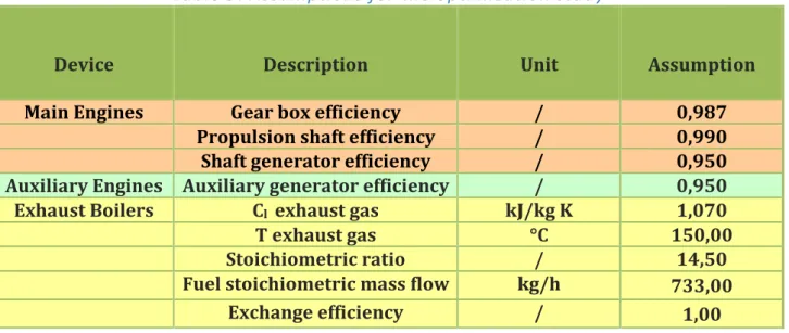
Heat balances, using the actual temperature of the seawater, estimate the thermal load. For "standard" consumption, exhaust boilers are widely enough, and moreover they have to download the excess steam [6]. A big consumption of heat is necessary for the cleaning of storage tanks between a load and the other. The consumption associated with heating of the load occurs very rarely, because generally both petroleum and chemists products have the right viscosity at ambient temperature. Cleaning storage tanks and heating loads requires the use of one auxiliary boiler [6]. There are two different configurations for the propulsion system. The first (Figure 1) is related to the shaft generator connected to the main engines (ME1, ME2); the second layout (Figure 2) refers to operation with auxiliary engines running (AE1, AE2).

The first layout can refer to "SG" since it makes use of the so-called "Shaft Generator", instead of the second one that refers to "AE" since it makes use of auxiliary engines [6].

The layout SG is basically the one used with greater frequency, since it allows the generation of current with higher efficiency. The main engines are in fact more efficient than the auxiliary ones [6].

However, this choice is made unconsciously by the operators, because in reality much depends on the load of the engines: it would be much more convenient for example, at low speed, working only with one main engine at full load with the electrical load deflected on the auxiliary engines, rather than working with two main motors at low load. In any case, unless something goes wrong, the SG

(13)

layout is always used when the tanker is sailing. Further use of it, it’s made during unloading of the load, since the power required can largely overcome the power provided by auxiliary motors [6]. The main use of AE is during the waiting in port (because the main engines are off), and whenever there is a problem with the main generator.

ME

1

ME

2

GEAR

BOX

Mechanical power (propulsion)

AE

1

AE

2 Electrical power Electrical power Electrical power SG AG AG

Figure 1: Layout “SG” – Shaft Generator

ME

1

ME

2

GEAR

BOX

Mechanical power (propulsion)

AE

1

AE

2 Electrical power Electrical power Electrical power SG AG AG

Figure 2: Layout “AE” – Auxiliary Engines

(14)

2. Selection of the Operational Phases

Understanding the origin of power request is very useful during an optimization analysis, because it can show in which points the system can be improved. Regarding the activity of a chemical tanker, the power request can swing significantly during its operative life [7], so it’s very useful dividing it in different phases. The available electrical balance, that is the list of all the electrical devices installed on board together with their consumption, suggests a division into 4 distinct stages [8]:

• Normal seagoing condition;

• Normal seagoing with ballasting, heating and cleaning; • Port cargo handling;

• Port in – port out.

During the “normal seagoing condition”, the chemical tanker sails loaded of goods: on the ship there are no particular activities [6]. This phase it’s very important for two reasons: it takes a large amount of time during the annual operation of the tanker and a large consumption of power is expected due to propulsion (this consumption varies as a function of speed).

The phase "normal seagoing with ballasting, heating and cleaning" is the phase in which the ship is travelling unloaded to reach the port in which it can take the new load. The wasted trip is called "ballast trip" or "ballast leg", hence the term "ballasting" [6]. During the ballast trip, it’s often necessary preparing the holds for the next load, cleaning them from the residues of the previous cargo (hence "cleaning"). This requires a high production of steam on board [6]. The term "heating" refers to the heating of load in the case it has a particular high density: this requires again the use of auxiliary boilers [6]. This phase it’s very important for two reasons: a large consumption of power is expected due to propulsion, furthermore there is higher consumption of electrical and thermal power than the normal seagoing condition (due to heating and cleaning on board). Although this phase indicates the whole travel during which the tanker is unloaded, hereinafter this phase will regard only cleaning and heating periods in navigation: with no heating and cleaning on board, the phase is considered of “normal seagoing condition”.

The port cargo handling is the phase characterized by the peaks in electrical consumption that occur in port, during the loading – unloading of goods: this stage is crucial for the optimization study. Finally, port in – port out is the phase of manoeuvre in port. However, this phase can be considered negligible since it takes very short time during the annual activity. Furthermore, this stage sometimes is put into account because many ships are equipped with bow propellers for manoeuvring, which have significant power consumption. This is not the case for the tanker under study, and consequently the consumption in this stage is very similar to the one of pure navigation. Looking at the excel sheet that describe the punctual consumption of the tanker, it’s possible to notice that there is another important stage to be considered: the waiting in port [7]. Although mechanical load is not requested and electrical and thermal ones are almost constant, this phase takes a large amount of time (almost half of the annual activity of the chemical tanker) [7].

In the light of these considerations, the following phases will be taken into account in the further analysis; abbreviations are going to be used for simplicity, as Table 1 shows:

(15)

Table 1: Abbreviations of the Operational Phases [6]

Operational Phase Abbreviation

Normal seagoing condition

‘FUL’

Normal seagoing with ballasting, heating and cleaning

‘BAL’

Port cargo handling

‘CAR’

Waiting in port

(16)

3. Comparison between Real and Design

Electrical Loads

It’s necessary verifying if electrical loads measured on the tanker are close to the ones calculated by the manufacturers; as previously said, this allows comprehending if devices installed on board are correctly estimated concerning the power they provide.

At the end of the list of all the electrical devices installed on board, the total power requested is indicated for each phase [8]. This data are simply an estimation of the designers concerning the electrical consumption on board during the four phases. However, for the waiting in port there are no data available, thus the check is made concerning the first three stages (FUL, BAL, CAR). Table 2 shows the estimation of requested power:

Table 2: Estimation of requested Power [8] Normal seagoing

condition (kW)

Normal seagoing with ballasting, heating and cleaning

(kW)

552,2 1273,9 3035,1

At first, it’s necessary making the division of all the four operational phases previously discussed also in the excel sheet which describes the punctual consumption of the chemical tanker in one year of activity.

In order to avoid problems related to the automatic association, every punctual value of power over the operational year is associated to one of the four main phases manually. Automatic association is possible but hazardous because it requires high knowledge about the energy system on board. This selection is made following some guidelines that are summarized below:

• The normal seagoing condition is characterized by request of propulsion load and with no particular activities that require an increase of electrical and thermal request of power. • The normal seagoing with ballasting, heating and cleaning has more demand of thermal

power than the previous phase; it requires propulsion load as well.

• The port cargo-handling phase is characterized by no propulsion and high demand of electrical power due to cargo operations.

• The waiting in port requires neither propulsion nor particular demand of electrical and thermal power.

After these considerations, it is feasible to associate every single value of power to one of these four main phases.

Subsequently this fundamental analysis, it is possible to compare the consumption estimated by the designers with the real energy consumption on the ship. The methodology to do that is summarized below:

(17)

• For the three phases considered (waiting in port is excluded), two operations are put into account: the first one is a mean value, the second one is the operation that requires the largest amount of power over the year.

• For both the operations, the punctual consumption of energy is calculated simply multiplying the value in kW by the amount of time considered (15 min.). Afterwards, the punctual consumptions of energy are summed. Therefore the real consumption of energy is obtained (for both the operations of the three phases).

• After that, the value of power previously estimated (Table 2) is multiplied by the amount of time that the two operations of the three phases require: the design consumption of energy is obtained.

• At the end, a ratio between the design and the real consumption of energy is calculated for both the operations of the three phases, as Table 3 shows:

Table 3: Ratio between Design and Real Energy consumption Operational phase Mean Operation (𝒅𝒆𝒔𝒊𝒈𝒏 𝒌𝑾𝒉 𝒓𝒆𝒂𝒍 𝒌𝑾𝒉 ) Most expensive Operation (𝒅𝒆𝒔𝒊𝒈𝒏 𝒌𝑾𝒉 𝒓𝒆𝒂𝒍 𝒌𝑾𝒉 )

Normal seagoing condition

1,60 1,49

Normal seagoing with ballasting, heating and cleaning

1,48 1,26

2,43 1,96

Table 3 shows a certain degree of safety for all the phases under study. Also in the most expensive operation, the energy consumption estimated by the manufacturers exceeds at least 26% the real one. Furthermore, the degree of safety seems not to overcome an excessive value: these facts suggest that the size of the electrical devices on board is well estimated.

(18)

4. Load’s curves for the Simulation

4.1 Calculation of Average Power values

A further crucial step is to obtain curves of mechanical, electrical and thermal power as a function of time for all the operational phases considered. The goal is to get power profiles that can be managed during the optimization stage.

With a simple filtering operation, it is possible to consider separately the four phases previously defined [7]. Information regarding thermal power demand for tank cleaning are not available, therefore this required power is going to be taken into account only from the optimization stage (chapter 5) and is going to be estimated on the basis of actual consumption of the ship.

Here, annual curves of mechanical, electrical and thermal loads related to the four phases are reported [7].

4.1.1 Normal Seagoing Condition

Figure 3: Annual Mechanical Power – ‘FUL’ phase [7]

(19)

Figure 5: Annual Thermal Power – ‘FUL’ phase [7]

4.1.2 Normal Seagoing with Ballasting, Heating and Cleaning

Figure 6: Annual Mechanical Power – ‘BAL’ phase [7]

Figure 7: Annual Electrical Power – ‘BAL’ phase [7]

(20)

Figure 8: Annual Thermal Power – ‘BAL’ phase [7]

4.1.3 Port Cargo – Handling

Figure 9: Annual Mechanical Power – ‘CAR’ phase [7]

Figure 10: Annual Electrical Power – ‘CAR’ phase [7]

(21)

Figure 11: Annual Thermal Power – ‘CAR’ phase [7]

4.1.4 Waiting in Port

Figure 12: Annual Mechanical Power – ’WAI’ phase [7]

Figure 13: Annual Electrical Power – ’WAI’ phase [7]

(22)

Figure 14: Annual Thermal Power – ’WAI’ phase [7]

4.1.5 Results

As Figures 3-14 show, most of the loads have almost a constant profile during the operational year [7]. This is advantageous for the optimization stage through software, because it allows managing power demands with simplicity. However, some of the loads previously shown are not constant over the range of time considered. They are:

• Mechanical load in normal seagoing condition;

• Mechanical load in normal seagoing with ballasting, heating and cleaning; • Electrical load in normal seagoing with ballasting, heating and cleaning; • Electrical load in port cargo – handling.

Mechanical loads swing due to speed regulation; instead electrical loads vary because of the different request of power necessary to perform operations as load handling [6].

It is possible calculating the average values of power related to the main four phases. Variable loads are underlined in yellow. As Table 4 suggests, thermal demand is almost constant over the whole operational year (tank cleaning is not included, as previously said). Furthermore, during the FUL phase, power demand is slightly greater than the one in BAL phase, because in normal seagoing condition the tanker is full of goods so, in order to maintain the same cruise speed, the requested power is higher than the case in which the tanker is empty (in BAL phase).

Table 4: Average Values of Requested Power over the four Main Phases (one year) [7]

Load ‘FUL’ ‘BAL’ ‘CAR’ ‘WAI’

Mechanical (kW) 4135 3803 0 0

Electrical (kW) 344 1081 1385 329

(23)

After that, it’s possible estimating energy consumption. The amount of hours related to all the four phases during one operational year is reported in Table 5. It is shown that FUL and WAI phases represent almost half operational time each one; BAL and CAR phases are one order of magnitude lower than the other two.

Table 5: Annual hours of the four phases [7]

‘FUL’ ‘BAL’ ‘CAR’ ‘WAI’

Annual hours (h) 4334 384 512 3550

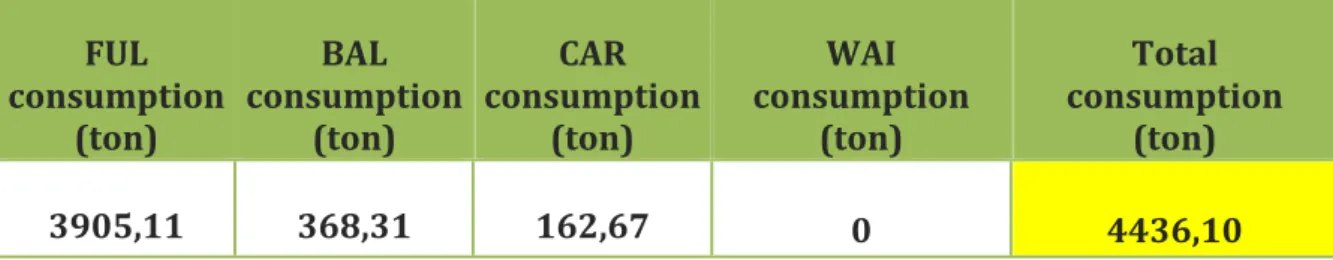
Then, energy consumption over one operational year is reported in Table 6. Main consumptions are mechanical ones, due to high demand of power for propulsion.

Table 6: Average Values of Annual Requested Energy over the four Main Phases [7]

Load ‘FUL’ ‘BAL’ ‘CAR’ ‘WAI’ Total

Mechanical (MWh) 17922 1460 0 0 19382

Electrical (MWh) 1489 415 709 1167 3780

Thermal (MWh) 1128 100 139 926 2293

4.2 Loads’ Distribution during the four Phases

The goal is obtaining power profiles that can be managed during the optimization phase through software. Sometimes average values don’t represent the real profile in a good manner, so it can be useful analysing the distribution of power request during one operational year, in order to estimate power inputs to be taken into account in the simulation. The range of power is chosen for all the four phases, depending on their fluctuation over the period considered. Once again, thermal power request for tank cleaning is not put into account, as previously explained.

Figures 15-24 below show the distribution of mechanical, electrical and thermal loads during the four phases (over one operational year); then, observations on the values of power request that must be considered in the optimization stage are proposed.

(24)

4.2.1 Mechanical load

Figure 15: Distribution of Mechanical load – ‘FUL’ phase [7]

Figure 16: Distribution of Mechanical load – ‘BAL’ phase [7]

4.2.2 Electrical load

Figure 17: Distribution of Electrical load – ‘FUL’ phase [7]

0 200 400 600 800 1000 0 -‐ 500 500 -‐ 1000 1000 -‐ 1500 1500 -‐ 2000 2000 -‐ 2500 2500 -‐ 3000 3000 -‐ 3500 3500 -‐ 4000 4000 -‐ 4500 4500 -‐ 5000 5000 -‐ 5500 5500 -‐ 6000 6000 -‐ 6500 6500 -‐ 7000 7000 -‐ 7500 Hours/year Range (kW)

'FUL' -‐ Distribution of Mechanical load

0 50 100 150 0 -‐ 500 500 -‐ 1000 1000 -‐ 1500 1500 -‐ 2000 2000 -‐ 2500 2500 -‐ 3000 3000 -‐ 3500 3500 -‐ 4000 4000 -‐ 4500 4500 -‐ 5000 5000 -‐ 5500 5500 -‐ 6000 6000 -‐ 6500 6500 -‐ 7000 Hours/year Range (kW)

'BAL' -‐ Distribution of Mechanical load

0 1000 2000 3000 4000 0 -‐ 100 100 -‐ 200 200 -‐ 300 300 -‐ 400 400 -‐ 500 500 -‐ 600 600 -‐ 700 700 -‐ 800 800 -‐ 900 900 -‐ 1000 Hours/year Range (kW)

(25)

Figure 18: Distribution of Electrical load – ‘BAL’ phase [7]

Figure 19: Distribution of Electrical load – ‘CAR’ phase [7]

Figure 20: Distribution of Electrical load – ‘WAI’ phase [7] 0 20 40 60 80 100 Hours/year Range (kW)

'BAL' -‐ Distribution of Electrical load

0 20 40 60 80 0 -‐ 1 00 10 0 -‐ 2 00 20 0 -‐ 3 00 30 0 -‐ 4 00 40 0 -‐ 5 00 50 0 -‐ 6 00 60 0 -‐ 7 00 70 0 -‐ 8 00 80 0 -‐ 9 00 90 0 -‐ 1 00 0 10 00 -‐ 11 00 -‐ 12 00 -‐ 13 00 -‐ 14 00 -‐ 15 00 -‐ 16 00 -‐ 17 00 -‐ 18 00 -‐ 19 00 -‐ 20 00 -‐ 21 00 -‐ 22 00 -‐ 24 00 -‐ 25 00 -‐ 26 00 -‐ 27 00 -‐ Hours/year Range (kW)

'CAR' -‐ Distribution of Electrical load

0 1000 2000 3000 0 -‐ 100 100 -‐ 200 200 -‐ 300 300 -‐ 400 400 -‐ 500 500 -‐ 600 600 -‐ 700 700 -‐ 800 800 -‐ 900 900 -‐ 1000 Hours/year Range (kW)

(26)

4.2.3 Thermal load

Figure 21: Distribution of Thermal load – ‘FUL’ phase [7]

Figure 22: Distribution of Thermal load – ‘BAL’ phase [7]

Figure 23: Distribution of Thermal load – ‘CAR’ phase [7]

0 500 1000 1500 2000 0 -‐ 20 20 -‐ 40 40 -‐ 60 60 -‐ 80 80 -‐ 100 100 -‐ 120 120 -‐ 140 140 -‐ 160 160 -‐ 180 180 -‐ 200 200 -‐ 220 220 -‐ 240 240 -‐ 260 260 -‐ 280 280 -‐ 300 300 -‐ 320 320 -‐ 340 340 -‐ 360 360 -‐ 380 Hours/year Range (kW)

'FUL' -‐ Distribution of Thermal load

'BAL' -‐ Distribution of Thermal load

(27)

Figure 24: Distribution of Thermal load – ‘WAI’ phase [7]

Mechanical load is not requested during the phases of ‘port-cargo handling’ and ‘waiting in port’, since there is no propulsion demand [6], so the distribution of load is not represented.

Figures 15-24 show different behaviours and situations that are going to be explained.

At first, there are few distributions that show high similarity to the profile of power estimated by the mean values found before. For instance, the distribution of the electrical load during the FUL phase reflects the result obtained by mean values: it was found that during this phase the mean value of requested power was 344 kW. Through the distribution of power, the same result is achieved: there is only one strong peak in the range of power 300-400 kW and other two little peaks in the previous and in the next ranges (200-300 kW and 400-500 kW). For this and a few other distributions, the calculated mean value of power is in accordance with the distribution study.

However, most of the cases demonstrate that the estimated mean value doesn’t reflect the real situation in a good way. In many loads the distribution is wide, so the profile of power must be represented in a different manner.

A solution that could allow manipulating and simulating the power profile is necessary; otherwise the study could become inaccurate. To solve the problem, the software Visual Basic Application (VBA) is used: it works with excel interface and it tries to find a solution to the problem. Its use is explained in the next section, together with the obtained results.

0 500 1000 1500 0 -‐ 20 20 -‐ 40 40 -‐ 60 60 -‐ 80 80 -‐ 100 100 -‐ 120 120 -‐ 140 140 -‐ 160 160 -‐ 180 180 -‐ 200 200 -‐ 220 220 -‐ 240 240 -‐ 260 260 -‐ 280 280 -‐ 300 300 -‐ 320 320 -‐ 340 340 -‐ 360 360 -‐ 380 Hours Range (kW)

(28)

4.3 Use of Visual Basic Application (VBA)

Through Visual Basic Application, an excel sheet is created in order to solve the problem related to those loads that show a wide distribution of power during the operational year.

Here, the logic of the spread sheet is explained: it is composed by different steps and it considers one single load of one single phase, so the procedure must be repeated for all the loads of all the phases under study. The most important characteristic of this sheet is to be adapted to all the ships and tankers that need an energy optimization, being useful not only for this particular treated case.

1. At first is possible to set values of requested power and number of hours that this request occurs during the year. This stage can be completed simply using values of power and number of hours considered in the previous distribution study. Mechanical load during the FUL phase may be considered as example. From the distribution study the request of power is divided into different ranges: all of them are characterized by a number of hour that represents the request of power that occurs in these ranges. Concerning the FUL phase, the ranges are developed every 500 kW; in order to identify each range with a single value, it’s possible to assume mean values as 250 kW (that identifies the range 0 – 500 kW), 750 kW (that identifies the range 500 – 1000 kW), etc. Finally it’s possible associating to each value of power the related number of hour representing the request of power that occurs in the same range. The sheet provides also the total number of hours related to the request of power of the load under study for the whole phase considered, together with the peak of power performed in the same phase.

2. After that, it’s possible to press the button “shake”, which provides the mixing of the entered values in a random order. This tool allows avoiding the creation of a profile with an increasing request of power (if the user set the inputs following the ascending order) and it permits to generalize the situation. However, if the case under study must be characterized by a certain sequence of values, the user, after the setting of values following the desired order, can escape the button “shake”, switching to the next step.

3. Subsequently, pressing the button “curve creation”, the profile of power is created. Every single hour is represented by a single value of power and the succession is shown in the excel sheet.

4. Finally, it’s possible setting the number of times the user wants to repeat the created profile during the year. The software modifies the profile maintaining the same amount of requested energy, regardless the number of times the profile is repeated. Increasing the number of time of the profile repetition, the calculation looses a certain amount of hour due to the inconvenience to consider the hours as decimal numbers. For instance, if a certain request of power lasts for 33 hours over the year and the user wants repeating the whole profile 10 times (during the same year), each of these profiles should be characterized by 3,3 hours of the same request of power. This is not convenient because the tool is set on kWh considering the hours as integers, hence the software takes into account the integer value (in this case 3 hours); the remaining part is spread over the whole year, together with the remaining parts of all the values of power considered.

Figure 25 shows the just described interface of the spread sheet, concerning the mechanical load of the FUL phase.

(29)

Figure 25: Interface of the spread sheet

The final goal of this stage is obtaining curves of mechanical, electrical and thermal loads over one year. Here, there are two different ways that can be crossed:

1) The phases under study (FUL, BAL, CAR, WAI) may be considered one after the other, as if the ship performs at first the whole phase of seagoing, then the whole phase of ballasting, then the whole phase of cargo and finally the whole phase of waiting in port. This approach is easy to be conducted; the energy point of view doesn’t care about the order of the phases, even during the next stage of optimization. However, there could be a problem if in the subsequent optimization a system of energy storage would be taken into account.

2) The second way considers a certain sequence of phases, repeating it a certain number of times during the operational year. This fact avoids the problem of energy storage mentioned in the first way, because it simulates a more real profile of requested power (the phases alternate with each other through a logical sequence). Putting into account an energy storage system, the more the profile of power is similar to the reality the more is possible to estimate with a great accuracy the periods during which it’s possible to accumulate energy and the periods during which this energy can be exploited.

The second way requires some hypothesis and it’s more difficult to be conducted than the first one; however it’s going to be chosen due to the possibility to consider an energy storage system in the further optimization.

The first decision is the choice of the sequence of phases that is going to be repeated over the operational year. This sequence is shown below [7]:

total%hours 4335

max%power%[kW] 7.250 4270

rows%considered 15 curve%repetition 10

Mean%power%[kW] total%hours/phase Mean%power%of%interest%[kW] total%hours/phase hours/repetition hours/10

1 1750 57 1750 57 5 0,5 1 1802 2 750 33 750 33 3 0,3 2 1802 3 6250 482 6250 482 48 4,8 3 1802 4 250 27 250 27 2 0,2 4 1802 5 3750 824 3750 824 82 8,2 5 1802 6 5250 157 5250 157 15 1,5 6 802 7 6750 90 6750 90 9 0,9 7 802 8 5750 180 5750 180 18 1,8 8 802 9 2250 59 2250 59 5 0,5 9 6302 10 2750 298 2750 298 29 2,9 10 6302 11 3250 710 3250 710 71 7,1 11 6302 12 4250 908 4250 908 90 9 12 6302 13 1250 91 1250 91 9 0,9 13 6302 14 7250 9 4750 410 41 4,1 14 6302 15 4750 410 0 15 6302 16 16 6302 17 17 6302 18 18 6302 19 19 6302 20 20 6302 21 21 6302 22 22 6302 23 23 6302 24 24 6302 25 25 6302 26 26 6302 27 27 6302 28 28 6302 29 29 6302 30 _+1000,0, 30 6302 1000, 2000, 3000, 4000, 5000, 6000, 7000, 8000, 0, 500, 1000, 1500, 2000, 2500, 3000, 3500, 4000, 4500, Curve,crea5on, _SHAKE,

(30)

1) WAI 2) CAR 3) BAL 4) CAR 5) FUL

After a phase of waiting in port, there is a phase of unloading of goods, followed by a ballast trip during which the holds are cleaned for the next load. After that, a loading phase is expected and finally the loaded ship performs a phase of seagoing towards the next destination, then the cycle restarts [7]. Obviously the sequence can be changed according to the requirements of the ship under study.

The second and final decision is to determine how many times this sequence must be repeated during the year. This choice depends on the activity of the ship over the year. For this tanker, the number of repetition is set to 10 [7]. Even in this case, the number of repetition can be changed. Figures 26-29 show mechanical, electrical and thermal loads over one year considering the sequence explained before and putting into account 10 repetitions of this sequence. These curves are going to be considered as input in the next optimization stage.

Figure 26: Mechanical load Profile over one operational year

(31)

Figure 28: Thermal load Profile over one operational year

Figure 29: Mechanical, Electrical and Thermal load Profiles over one operational year

After the approximation of these curves, an accuracy check is needed. The parameter that is able to show the precision of the results is the produced energy. A comparison between the energy provided by the obtained curves and the real ones is necessary. In both the cases of thermal load, tank-cleaning contribution is missing and is going to be considered in the next chapter. Table 7 below proves that the difference is always less then 1%, so the optimization can be performed through the achieved model curves. This difference is due to the approximation made during the choice of the ranges of power and particularly considering a mean value as representative of each range of power (in other words the assumptions made in step 1 of section 4.3).

Table 7: Energy check

Energy check Mechanical load _(kWh) Electrical load _(kWh) Thermal load _(kWh)

Obtained Curves 19 447 500 3 751 000 2 288 800

Real Curves 19 380 779 3 783 027 2 295 719

(32)

5. Optimization of the on-‐board Energy

System

5.1 Assumptions

At the beginning of this analysis it’s fundamental identifying which devices work during the four phases (FUL, BAL, CAR, WAI). Table 8 shows the situation:

Table 8: Devices for Energy Production on-‐board [6]

Phase Mechanical Energy

Electrical Energy

Thermal Energy

FUL Main Engines Shaft Generator Exhaust Boilers

BAL Main Engines Shaft Generator Exhaust Boilers + Auxiliary _Boilers

CAR Main Engines Shaft Generator Exhaust Boilers

WAI Auxiliary Engines Auxiliary Generator Auxiliary Boilers

Some of these considerations are obvious; other ones are the result of a rational reasoning.

In the FUL phase, the main engines and the shaft generator produce mechanical and electrical power respectively; exhaust boilers are enough for thermal power due to its low request during the normal seagoing [6].

In the BAL phase, the main engines and the shaft generator produce mechanical and electrical power as well; here, because of the high request of thermal power due to operations as tank cleaning, exhaust boilers are not sufficient and they are helped by auxiliary boilers [6].

In the CAR phase, even if the ship is not sailing, the main engines are on and the shaft generator produce electrical power; this is a reasonable approximation because during the cargo there are some peaks of electrical request of power that cannot be provided by the auxiliary engines [6]. Also in this case, exhaust boilers are enough for thermal power due to its low request [6].

In the WAI phase, main engines are off, so the auxiliary engines and the auxiliary generator produce mechanical and electrical power respectively. Auxiliary boilers provide thermal request of power [6].

After this fundamental overview, it’s necessary defining some assumptions that will characterize the optimization study. Table 9 shows the hypothesis made: