ALMA MATER STUDIORUM
UNIVERSITA’ DI BOLOGNA
S
CUOLA DI
I
NGEGNERIA E
A
RCHITETTURA
Sede di Forlì
Corso di Laurea Magistrale in
I
NGEGNERIA
A
EROSPAZIALE
Classe 8197
T
ESI DI LAUREA
In
D
INAMICA E CONTROLLO ORBITALE LM
Magnetic Actuators for Nanosatellite Attitude Control
C
ANDIDATO
R
ELATORE
Niccolò Bellini
Prof. Paolo Tortora
C
ORRELATORE
Prof. Jordi Puig-Suari
Anno Accademico 2013/2014
Sessione
II
1
Abstract
La ricerca e le attività presentate nella seguente relazione di tesi sono state condotte presso il California Polytechnic State University (USA) sotto la supervisione del Prof. Jordi Puig Suari.
L'obiettivo della ricerca ha riguardato lo studio di attuatori magnetici, comunemente chiamati magnetorquer, per il controllo di assetto di nanosatelliti. Tali attuatori si dividono generalmente in tre diverse tipologie: avvolgimenti air-core, avvolgimenti integrati e torquerod. Si tratta di dispositivi che, alimentati con modeste quantità di corrente, permettono di generare un campo magnetico il quale, interagendo col campo magnetico terrestre, può essere controllato per imprimere determinate rotazioni al satellite effettuando così manovre di puntamento.
In una prima fase dell'attività, ogni tecnologia è stata analizzata, definendo vantaggi e svantaggi, studiando le procedure di fabbricazione, ricavando equazioni per il dimensionamento basate su modelli matematici del comportamento fisico. Questi ultimi sono stati implementate in software numerici per creare uno strumento che permettesse di determinare la configurazione ottimale in base a determinati vincoli e specifiche di input.
In una seconda fase delle attività i modelli creati sono stati validati sfruttando prototipi già esistenti e realizzandone di nuovi. Sono dunque state effettuate misure delle grandezze caratteristiche di tali attuatori che permettessero un confronto tra il comportamento reale e quello teorico. Gli strumenti e il materiale sfruttati per esperimenti e prototipi sono stati forniti dai laboratori PolySat e CubeSat.
I risultati ottenuti hanno portato alla creazione di routines di dimensionamento complete per la progettazione di tali dispositivi e alla definizione di una procedura di design basata sulla completa libertà di scelta di tutti i parametri. Oltre a ciò è stata fatta anche un'analisi approfondita dei costi per ogni tipo di soluzione.
I modelli e gli strumenti sono stati mantenuti completamente parametrici per offrire la possibilità di riscalare tali tipi di attuatori per satelliti di classe e dimesione diversa.
3
Abstract
The research and the activities presented in the following thesis report have been led at the California Polytechnic State University (US) under the supervision of Prof. Jordi Puig Suari.
The objective of the research has been the study of magnetic actuators for nanosatellite attitude control, called magnetorquer. Theese actuators are generally divided in three different kinds: air core torquer, embedded coil and torquerod. In a first phase of the activity, each technology has been analyzed, defining advantages and disadvantages, determining manufacturing procedures and creating mathematical model and designing equation. Dimensioning tools have been then implemented in numerical software to create an instrument that permits to determine the optimal configuration for defined requirements and constraints.
In a second phase of the activities the models created have been validated exploiting prototypes and proper instruments for measurements. The instruments and the material exploited for experiments and prototyping have been provided by the PolySat and CubeSat laboratories.
The results obtained led to the definition of a complete designing tool and procedure for nanosatellite magnetic actuators, introducing a cost analysis for each kind of solution.
The models and the tools have been maintained fully parametric in order to offer a universal re-scalable instrument for satellite of different dimension class.
5
Index
1.Nanosatellite Attitude Control System ... 10
1.1 Magnetorquer ... 11
1.2 Magnetorquer design parameter ... 14
1.2.1 Generated Dipole ... 14
1.2.2 Mass ... 14
1.2.3 Power Consumption ... 15
1.3 Magnetorquer Designing procedure ... 16
2. Fundamentals of Magnetism ... 18
2.1 Magnetic field strength and magnetic flux density... 18
2.2 Magnetization ... 19
2.3 The demagnetizing factor ... 22
2.4 Diamagnetic Materials ... 23
2.5 Paramagnetic Materials ... 24
2.6 Ferromagnetic Materials ... 25
2.6.1 Hysteresis Cycle ... 25
2.6.2 Magnetic anisotropy ... 27
2.6.3 Soft and hard ferromagnetism ... 28
2.6.4 Temperature influence ... 30
2.6.5 Eddy Current ... 30
3. Embedded coil ... 32
3.1 Description and manufacturing ... 32
3.2 Model ... 33
3.2.1 Magnetic dipole ... 33
3.2.2 Balanced spiral in multilayer magnetorquer ... 39
3.2.3 Magnetic field strength ... 40
3.3 Designing issues ... 44
3.4 Experimental measures on embedded coil ... 48
3.4.1 No Solar cell mounted panel ... 53
3.4.2 Solar cell mounted panel ... 55
3.4.3 Comparison between the two case ... 59
3.4.7 Corrective parameters ... 61
6
4.1 Description and Manufacturing ... 67
4.2 Model ... 68
4.2 Designing issues ... 68
4.7 Experimental measures on air core magnetorquer ... 76
4.7.1 No Solar Cell mounted Panel ... 78
4.7.2 Solar Cell Mounted Panel ... 80
4.7.3 Comparison between the two case ... 81
4.7.4 Corrective parameters ... 84
5. Torquerod magnetorquer ... 88
5.1 Description and Manufacturing ... 88
5.2 Torquerod Designing issues ... 89
5.2.1 Demagnetization Issues ... 90
5.2.2 Mass ... 93
5.2.3 Control mode ... 94
5.2.4 Choice of the core material ... 95
5.3 Dimensioning equation for torquerod ... 99
5.4 Experimental measures on torquerod prototype ... 116
6. Design of a 3axis torquerod for CubeSat ... 127
7. Magnetorquer preliminary design ... 135
8. Cost Analysis ... 146
9. Conclusion ... 148
7
Table of Figures
Fig. 1 Magnetorquer basic principle of operation [4] ... 12
Fig. 2 Principle of operation of a solenoid without core [6] ... 18
Fig. 3 Magnetization tends to align the magnetic dipole depending to the external applied field [6] ... 21
Fig. 4 Paramagnetic and diamagnetic materials behavior [6] ... 24
Fig. 5 Domains orientation in a ferromagnetic sample [6] ... 26
Fig. 6 Typical hysteresis cycle of ferromagnets [6] ... 27
Fig. 7 Iron and Nickel crystal hysteresis cycle [6] ... 28
Fig. 8 Example of easy and hard magnetizations according to crystallographic orientation [6] ... 28
Fig. 9 Hard and soft ferromagnetic hysteresis cycle [6] ... 29
Fig. 10 Example of commercial embedded coil for CubeSat application [8] ... 32
Fig. 11 Schematic example of square spiral embedded coil surrounded by magnetic field ... 33
Fig. 12 The torque (in yellow) tends to align the normal direction with the magnetic field ... 35
Fig. 13 Schematization of square spiral for embedded coil analysis ... 37
Fig. 14 Comparison between the simplified model and the spiral model ... 38
Fig. 15 Possible scheme of balanced multilayer embedded coil ... 39
Fig. 16 Square spiral scheme for H field analysis ... 40
Fig. 17 Square spiral scheme for H field analysis. Same colored segments give equal contribute ... 42
Fig. 18 Comparison between simplified model and spiral model for the H field estimation... 44
Fig. 19 Magnetic dipole reduction due to increase of spiral concentration ... 46
Fig. 20 Power consumption for a multilayer embedded coil ... 47
Fig. 21 Estimated mass increase for multilayer embedded coil ... 48
Fig. 22 Helmholtz cage exploited for embedded coil experimental measurements ... 51
Fig. 23 Embedded coil experimental layout ... 51
Fig. 24 Current Profile 1 ... 52
Fig. 25 Current Profile 2 ... 52
Fig. 26 No-solar cells mounted panel layout (photo 1) ... 53
Fig. 27 N-solar cells mounted panel layout (photo 2) ... 53
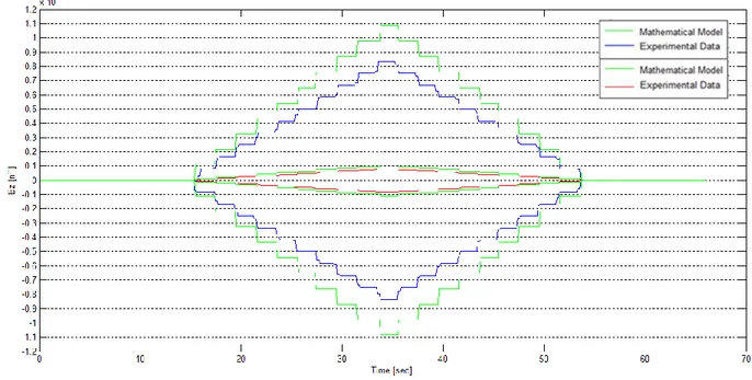
Fig. 28 Magnetic Flux in z direction for no-solar cells mounted panel ... 54
Fig. 29 Comparison between positive and negative magnetic flux profile ... 55
Fig. 30 Solar cells mounted panel experiment layout ... 56
Fig. 31 No-solar cells mounted panel cage calibration result ... 56
Fig. 32 Solar cells mounted panels cage calibration result ... 57
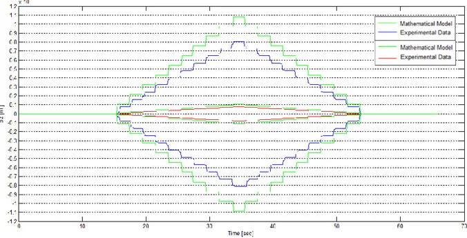
Fig. 33 Magnetic flux in z direction for solar cells mounted panel. ... 58
Fig. 34 Comparison between positive and negative magnetic flux profile for solar cells mounted panel ... 58
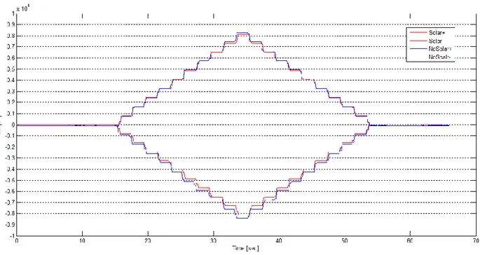
Fig. 35 Comparison between magnetic flux for solar cells and No-solar cells mounted panel (Profile 1) ... 59
Fig. 36 Magnetic flux difference between the solar cell case and no solar cells case(Profile 1) ... 60
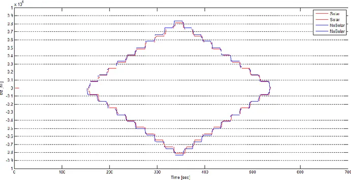
Fig. 37 Comparison between magnetic flux for solar cells and No-solar cells mounted panel (Profile 2) ... 60
Fig. 38 Magnetic flux difference between the solar cell case and no solar cells case(Profile 2) ... 61
Fig. 39 Evaluated artificial permeability from experimental results ... 62
Fig. 40 Ratio between the artificial permeability in the two case (Solar cells / No-solar cells) ... 63
8
Fig. 42 Expected dipole and adverse dipole evaluation ... 65
Fig. 43 Example of air core magnetorquer [11] ... 67
Fig. 44 Magnetic dipole variation depending on wire's diameter ... 70
Fig. 45 Power consumption model ... 71
Fig. 46 Mass model ... 71
Fig. 47 Magnetorquer 1 expected performances ... 72
Fig. 48 Magnetorqeur 2 expected performances ... 73
Fig. 49 Magnetorquer 3 expected performances ... 73
Fig. 50 Effective dipole corrective factor ... 75
Fig. 51 Air core magnetorquer prototype exploited for measurements ... 76
Fig. 52 Air core magnetorquer mounted on the panel ... 76
Fig. 53 Air core experimental setup ... 76
Fig. 54 Air core magnetorquer prototype expected performances ... 77
Fig. 55 Current profile 1 (Air Core experiment) ... 78
Fig. 56 Current profile 2 (Air Core experiment) ... 78
Fig. 57 Magnetic Flux in z direction for profile 1with no solar cells mounted ... 79
Fig. 58 Magnetic flux in z direction for profile 2 with no solar cells mounted. ... 80
Fig. 59 Magnetic flux in z direction for profile 1 with solar cells mounted ... 80
Fig. 60 Magnetic flux in z direction for profile 2 with solar cells mounted.. ... 81
Fig. 61 Comparison between solar cell and no solar cells mounted (Profile 1) ... 82
Fig. 62 Magnetic flux difference between the two case (Profile 1) ... 82
Fig. 63 Comparison between solar cell and no solar cells mounted (Profile 2). ... 83
Fig. 64 Magnetic flux difference between the two case (Profile 2) ... 83
Fig. 65 Evaluated permeability for air core experiment (Profile 1) ... 84
Fig. 66 Evaluated permeability for air core experiment (Profile 2) ... 85
Fig. 67 Ratio between the artificial permeability in the two case (Solar cells / No-solar cells) - profile 2 ... 86
Fig. 68 Ratio between the artificial permeability in the two case (Solar cells / No-solar cells) - profile 1 ... 86
Fig. 69 Example of minor hysteresis cycles [12] ... 91
Fig. 70 Demagnetizing slope [12] ... 92
Fig. 71 Example of apparent demagnetization exploiting minor hysteresis cycle [12] ... 93
Fig. 72 Resume table for main ferromagnetic materials [13] ... 96
Fig. 73 Magnifer 7904 characteristic slope [16] ... 98
Fig. 74 Magnifer 7904 permeability variation with respect to frequency [16] ... 98
Fig. 75 Demagnetizing factor dependence on L/r ratio ... 101
Fig. 76 Geometric parameter for different volumes of the core ... 103
Fig. 77 Alloy 79 first magnetization curve [16] ... 104
Fig. 78 Magnetic dipole dependence for different core’s shape ... 105
Fig. 79 Power consumption dependence for different core's shape ... 106
Fig. 80 Magnetic dipole and power consumption magnitude for different core's shape. ... 107
Fig. 81 Mass relation depending on core's shape ... 108
Fig. 82 Example of magnetic flux density for a defined core (10x80mm) ... 110
Fig. 83 Example of magnetic flux density for a defined core (7x80mm) ... 111
9
Fig. 85 Power consumption relation for different wire’s diameter (10x80mm) ... 113
Fig. 86 Magnetic dipole relation (10x80mm) ... 113
Fig. 87 Relation between magnetic flux and intrinsic magnetization [12] ... 114
Fig. 88 Ferrite core hysteresis loop reconstruction at 100 KHz ... 118
Fig. 89 Torquerod prototye design (1) ... 118
Fig. 90 Torquerod prototype design (2) ... 118
Fig. 91 Realized prototype (1)... 119
Fig. 92 Realized prototype (2)... 119
Fig. 93 Experiment layout scheme ... 121
Fig. 94 Experiment layout ... 122
Fig. 95 Current profile for torquerod experiment ... 122
Fig. 96 Magnetic flux density in x direction; experimental results and mathematical model ... 123
Fig. 97 Evaluated operative region during experiment ... 124
Fig. 98 Remanence of the core (measured in experiment configuration) ... 125
Fig. 99 Evaluated remanence inside the core ... 126
Fig. 100 Air core magnetorquer integration ... 127
Fig. 101 Embedded magnetorquer integration [8] ... 127
Fig. 102 Air core and embedded magnetorquer average encumbrance ... 128
Fig. 103 Designed torquerod integrated in CubeSat structure (1) ... 130
Fig. 104 Designed torquerod integrated in CubeSat structure (2) ... 130
Fig. 105 Optimal wire's diameter evaluation ... 131
Fig. 106 Performances for 0.3 mm wire's diameter ... 132
Fig. 107 Different possible performances for different wire's diameter @3.3V ... 133
Fig. 108 Different possible performances for different wire's diameter @5V ... 133
Fig. 109 Operative range for different designs (850 turns and variable wire's diameter) ... 134
Fig. 110 Magnetorquer optimal design procedure ... 137
Fig. 111 Design 1 AirCore ... 139
Fig. 112 Design 2 AirCore ... 139
Fig. 113 Design 3 AirCore ... 140
Fig. 114 Design 4 AirCore ... 140
Fig. 115 Design 5 AirCore ... 140
Fig. 116 Design 1 EmbeddedCoil ... 142
Fig. 117 Design 2 EmbeddedCoil ... 142
Fig. 118 Design 3 EmbeddedCoil ... 142
Fig. 119 Design 4 EmbeddedCoil ... 143
10
1. Nanosatellite Attitude Control System
Satellites for space application are divided in different category according to their mass. It’s considered a nanosatellite a satellite whose mass is below 10 Kg, while a microsatellite a satellite has mass which doesn’t exceed 50 Kg.
Among the first, one of the most famous is the CubeSat [1]: this kind of nanosatellite has been standardized in 2003 by prof. Jordi Puig Suari with the intent to offer the access to space to University and research institute exploiting a low cost platform. A CubeSat has in fact standard dimensions and size (100x100x100 – 1KG) and the cost for the launch results drastically reduced. Due to its versatility and simplicity, the CubeSat became the most launched satellite during the last years becoming one of the main commercial platforms for space application. Generally, due to its reduced dimensions and mass, CubeSat subsystems are often critical aspects and performances optimization is crucial: the few available power and volume pose many limitations to the use of certain technologies for subsystems.
Among these, most of nano and micro satellites need an appropriate attitude control system (ACS) that permits to the satellite to perform maneuver, fundamental for mission operations in orbit [2] [3].
For example, every satellite with a directional instrument, such as antenna or camera, need to be accurately oriented on target. Although, many satellite need to compensate torque disturbances to perform their task
Therefore, it is clear that ACS is an essential subsystem that must be carefully chosen and evaluated in the design phase of the mission. Furthermore, when the constraints are very stringent it is necessary that such a system is designed in an optimal way in order to avoid waste in terms of mass, volume and power consumption. There are multiple possible choices to design the ACS subsystem, exploiting different technologies and consisting mostly in two different categories: active controls (momentum wheels, magnetic dipole, and propulsion) and passive controls (gravity gradient boom, aerodynamic devices).
Passive control permits to impose the attitude of the satellite without controlling it directly according to the need: they provide stabilization in a defined attitude that can’t be changed during mission operation. The advantage of these devices consists in the fact that they do not require power to the satellite but do not offer
11
any flexibility. An example is a gravity gradient boom that forces the satellite to align with the radial direction of the earth, or permanent magnets that permits to align the satellite continuously in the direction of earth magnetic field.
On the contrary, active controls consist in real controls that permit to decide and change the attitude during on orbit operation according to the need. These kinds of devices request a power supply and control algorithm to work and for that reason their design represents one the most critical aspect of the whole satellite development. Reaction wheels consist of wheels that allow to transfer momentum to the satellite and to control its rotation: these are devices with masses and volumes that are not negligible and therefore very sensitive from a design point of view. Propulsion systems exploit a pressurized propellant that through appropriate nozzles allows even in this case to induce rotations and angular velocities with respect to the center of gravity of the satellite itself. Even in this case, the presence of tanks and pressurized substances poses great limits above all in nanosatellite application.
The last kind of active control is the so called magnetorquer. These kinds of control that will be deeply analyzed in this project are the more compact solution for nano and microsatellites, presenting both advantages and disadvantages with respect to the other devices presented.
1.1 Magnetorquer
A magnetorquer or magnetic torquer is a system for attitude control, detumbling and stabilization, based on the interaction between a generated magnetic dipole and earth magnetic field [2]. Through this interaction is generated a torque that is used to control the rotation of the satellite around is gravity center.
A magnetorquer is built using electromagnetic coils. When the coil is subject to a current generates the magnetic dipole control. This is a vector whose intensity is strictly connected to the geometry and the current provided. In the easiest case of a simple wounded coil this is expressed by the following formula:
Where m is the magnetic dipole intensity (measured in Am2), S is the area of the coil and n is the number of turns for a simply wounded coil. The direction of the
12
magnetic dipole is aligned with the axes of the coil and depending to the verse of the current.
The dipole tends to align with the external magnetic field environment or in our case the Earth's magnetic field. Since the dipole is rigidly bounded with the satellite, this is oriented accordingly.
The two parameters that determine the control are the direction of the torque vector and its intensity.
The torque vector is expressed by the formula:
⃗ ⃗⃗ ⃗
Where T is the torque, m is the magnetic dipole, and B is the external magnetic field.
The vector of the torque generated lies always in the plane of the coil and is perpendicular to the vector of the external magnetic field (Fig. 1). Therefore, in order to fully control the orientation and generate a torque vector with arbitrary direction, it is required to exploit 3 magnetorquer placed perpendicular. Nevertheless, in some circumstances could be required to control only one or two degree of freedom, reducing the number of needed magnetorquer and the complexity of the control law.
13
The intensity of the controlling torque depends on the intensity of the dipole, the intensity of the magnetic field and their respective orientation, thus being maximum when the dipole generated and the external magnetic field are perpendicular, then vanish once aligned.
The advantage of this kind of technology is linked to easy construction, high reliability, small mass and small power consumption, making it suitable for nanosatellite application. Considering that for the functionality isn't needed any kind of propellant, they are a resource always potentially usable as long as solar panels can provide a current.
Among disadvantages it appears clear that the functionality of the system strictly depends both on the efficiency of the magnetorquer its self, both on the external magnetic field that, for the earth magnetic field case, decreases moving to higher orbits: it means that in order to have appreciable torque at high altitude it would be required to have really high dipole intensity that means really high current with consequent high power consumption.
Generally the torques provided are very small and not sufficient in case of really accurate and fast orientation, differently than momentum wheels and propulsion. There are substantially three kind of magnetorquer:
Embedded magnetorquer: This magnetorquer is obtained directly on the PCB design and the wire is substitute by the copper trace of the board. The shape of the coil is a square spiral on a plane.
Air Core Magnetorquer: this magnetorquer consists in a certain number of turns of wire wrapped in wide circles. They are called "air core" because there is no material placed in the interior. Are usually installed in the side panels of the satellites.
Torquerod Magnetorquer: although the principle is the same of the air core magnetorquer, in this case, the winding is made in the form of a solenoid and in the volume contained by the coils is introduced a certain material with magnetic properties which amplifies the effectiveness of the device.
14
1.2 Magnetorquer design parameter
There are several aspects that are to be considered designing a magnetorquer. These issues have to respect the constraints and the requirements of the mission:
Generated dipole
Mass
Power Consumption
Occupied volume and interference
1.2.1 Generated Dipole
This is of course one of the most important features of the magnetorquer because it determines the efficiency of the control torque. The generated dipole cannot be determined arbitrarily, but must be determined in the design phase taking into account the key performance of the mission. Oversize the dipole has a significant impact on the budgets of mass and power available for attitude control subsystem of a satellite. These can be seen in the formula:
This general formula is exacted for air core magnetorquer, an approximation for embedded coil, and not applicable for torquerod. A higher requested momentum consists in higher current (consumption increase) or bigger area and turns (increase mass). It's important to evaluate the needed momentum to satisfy mission requirements in order to find the correct compromise.
1.2.2 Mass
As already said, both the number of turns and the area of the coil affect the total mass of the magnetorquer.
It can be possible to evaluate the mass of the wounded wire knowing the length and the size of the wire:
15
Where is the density of wire's material, is the area of the cross section L is the total length.
Increasing the area of the coil would cost in terms of total length and so in terms of total mass.
In general:
Where C is the length of a single coil and n the number of turns [5].
C is directly connected to shape of the coil. For a fixed mass and size it would be useful to increase the number of turns reducing wire diameter. On one side this could help to increase the generated dipole, but it would costs in term of power consumption.
Besides that each magnetorquer needs proper support structure: for embedded coil this consists in the PCB substrate while for air core and torquerod there are proper structure with different mass and dimensions.
For torquerod the total mass is affected also by the presence of the metal core that represent the bigger percentage.
1.2.3 Power Consumption
The power consumption of the coil is connected to the total resistance of the wire. This is due to two main factors: the resistivity of the wire's material, the cross section of the wire and its total length.
Where is the resistivity of wire's material and R the total resistance. The power consumption can be expressed as
Where R is the resistance, I is the current across the wire and P is the power absorbed.
16
The resistance is function of the temperature of the conductor and tend to decrease with the increase of the temperature. That means that, if the magnetorquer is driven with a constant voltage it’s important to perform a thermal analysis expecting some fluctuation on the current across it and in that way the magnetic dipole. In following analysis this aspect won’t be taken into account because strictly depend to the operative regime of the device and external condition.
As already said, increasing the current would increase significantly the power consumption, and the same increasing the resistance. Expressing the dependence of the power from the wire dimension it's possibly to put on evidence that the choice of wire diameter directly affects the performance of the device.
1.3 Magnetorquer Designing procedure
As presented, a magnetorquer is characterized by the power consumption, its mass, its dimension and of course the generated dipole. These aspects are strictly connected and it's always necessary to find the best compromise between the minimum performance required and the maximum power and dimensional budget. It's really important to define the main constraints for the system in order to have a starting input for the system optimization. It's not possible to define a universal strategy to obtain the best compromise because each mission or each scenario can be driven by different constraints that could lead to completely different choice. Generally, for a nanosatellite mission, especially for a CubeSat, one of the starting points is the needed torque: this come from evaluation concerning the requested pointing or despinning time and desaturation efficiency of the system. Through the definition of these specifics it's possible to define the requested magnetic dipole as a key performance parameter.
Concerning the constraints of the system, one of the most important can be the available power dedicated to the system: generally in fact, power budget is one of the most delicate aspects of each nanosatellite mission considering also that batteries are limited in Ampere per hour availability.
To define a designing strategy it's necessary to fix some inputs that permit to generate different solution depending to the variability of the other parameter. The
17
methodology that will be presented for all kind of magnetorquer will exploit as initial input the dimensions of the system and the nominal voltage supply. This choice seems quite logical since the area of the magnetorquer defined by its dimensions is the parameter that, in proportion, affects less the others maximizing the magnetic dipole that is the reason for which the system is designed. Especially considering the small size of a CubeSat it is not uncommon to be in a situation of forced dimensions for a subsystem, and exploiting the maximum available dimension is the most obvious solution to achieve the best performances. The voltage supply instead is a parameter that is almost standard depending to the class of the satellite (3.3 or 5 V for CubeSat), being the most of subsystem designed for standard voltage input and output.
The procedure will be fully parametric in every single variable: this allows to rescale the design for every satellite classes, from 1 to 50 Kg, simply changing the parameters.
To define properly the methodology and make it applicable to every kind of magnetorquer it's necessary to obtain a mathematical model (equations) for the design for each technology. To do that, a study of the magnetic properties involved is necessary, especially for the torquerod system. Where possible, the model obtained needs to be compared with real data from experimental results to validate it and to understand eventual unexpected issues.
18
2. Fundamentals of Magnetism
2.1 Magnetic field strength and magnetic flux density
As well known, every conductive wire crossed by a current induces in the nearest space a magnetic field. This, depending on the medium in this space determines a magnetic flux density. The magnitude and the direction of the magnetic field, variable in space, depend to the geometry of the structure that carry the current and the current intensity.
Taking in consideration a solenoid as example (Fig. 2), the magnetic field is constant in the inner volume and the strength is expressed by the formula [6]:
Where N is the number of turns, I the intensity of the current, and l the length of the solenoid. The unit of the magnetic field H is Ampere per meter (A/m).
The magnetic induction, or magnetic flux density, denoted by B and measured in Tesla, represents the magnitude of the internal field strength within a substance that is subjected to an H field. Both B and H are field vectors, being characterized not only by magnitude, but also by direction in space.
Fig. 2 Principle of operation of a solenoid without core [6]
19
µ represents the permeability of the medium and it's a property of the specific material through which H passes. Permeability is measured in H/m.
For a solenoid without metal core (assumed in vacuum)
Where is a universal constant equal to 1.25710-6
H/m.
When we introduce a core bar in the solenoid we substantially change the permeability of the medium.
The resulting Magnetic Flux density change and become
Where M is called magnetization. The presence of the core subjected to a magnetic field H reinforce the magnetic flux density B. The term is a measure of the contribution of the core.
2.2 Magnetization
Magnetization can be seen as the vector field that expresses the density of magnetic dipole moments in a material.
Magnetic dipole moments at atomic level are due to two different contributes: the first is the orbit of the electron around the nucleus that, being a moving charge, behave like a small current loop. The second contribution is due to electron spin along his axes. This spin magnetic moment can be in "up" direction or "down" direction [6].
In a single atom, the different magnetic moment due to orbital loop and spin may cancel each other’s. We call net magnetic moment the sum of all the magnetic moment contribution, spin and orbital, taking into account the eventual moment cancellation.
20
The net magnetic moment is strictly connected to the filling of atom's shells: for an atom having completely filled electron shells or subshells, when all electrons are considered, there is total cancellation of both
orbital and spin moments.
That's why these kinds of materials composed by these kinds of atoms can’t be permanently magnetized.
We can then define different types of magnetism: diamagnetism, paramagnetism, and ferromagnetism:
Diamagnetic materials show a weak magnetization with verse opposite to the external magnetic fields. For that reason these materials are not suitable at all to increase the magnetic dipole thus they weakly reduce it.
Paramagnetism on the contrary is the property of certain material to be weakly magnetized in presence of an external magnetic field in the same direction of it: this kind of magnetization doesn't persist without the external field and completely disappear when the exciting field is removed.
Ferromagnetism is the property of certain material to be strongly magnetized in presence of an external magnetic field and maintain the magnetization even when the external field is removed. They generally follow a hysteresis cycle, and for that reason it's not possible to find a linear and constant law to determine the intensity of the phenomena.
For the application studied it appears obvious that diamagnetism isn't the right solution, while paramagnetic and ferromagnetic materials are the possible solution that could be used to improve the efficiency of a magnetorquer, both with advantages and disadvantages.
As already said, magnetization is the vector that represents the density of magnetic dipoles moment in a material, both permanent and induced (Fig. 3).
An easy definition of magnetization is expressed by the formula
Where M represents magnetization, m is the vector that defines the magnetic moment, V represents volume and N is the number of magnetic moments in the sample. The quantity N/V is usually written as n, the number density of magnetic moments. The M-field is measured in amperes per meter (A/m) in SI units.
21
Fig. 3 Magnetization tends to align the magnetic dipole depending to the external applied field [6]
Another interesting expression for M is given by the following formula
over represents the variation of momentum over volume. In this expression M represent the density of dipole in a certain volume τ.
When M is constant in the medium we call it uniform magnetization.
We can understand the formula thinking about a cylinder shared in many slice, each with height dz. Each slide is shared in equal portion with area da. Then each prism with volume has a dipole oriented according to M that is the total magnetization. So we can consider:
Integrating over all the volume we can obtain the total dipole of the medium. In fact, M is measured in A/m that multiplied for a volume gives Am2 that is a magnetic dipole.
This relation is important because, once defined a magnetization M (depending on the material properties and external field) it's possible to determine the induced dipole of the medium.
A useful relation between M and H exists:
22
Where is the volume magnetic subscptibility, a dimensionless quantity. Taking in consideration the formula:
We can rewrite Where
is called relative permeability of the material; µ is called magnetic permeability of the material.
The relation is correct for diamagnetic and paramagnetic materials, while for ferromagnetism it's not possible to find a linear relation because of the magnetic hysteresis phenomena.
2.3 The demagnetizing factor
The magnetic behavior of samples does not only depend on its intrinsic properties but also on its shape and dimensions. The surface of a magnetic sample and the volume magnetic pole density generate an Hd field that tends to reduce the magnetization. The Hd field is called stray field [7].
When an external magnetic field is applied, the total magnetic field in a certain point is equal to
23
The H field is reduced due to the presence of the core of a quantity that is related to the magnetization.
The demagnetizing factor is the parameter that relates the stray field to the shape and the dimension of the ferromagnetic core.
The average volume magnetization of a sample is related to the demagnetizing field Hd
Where Nd is the demagnetizing tensor. For some samples in which the Ha field is applied according to the principal direction of the samples the two fields can be assumed parallel and the tensor is reduced to a scalar factor called in fact demagnetizing factor [7].
The effect could be understood in a simplified way taking in consideration the magnetic flux density B of the core:
Rewriting B
Where H is the H field induced with the presence of the core
The core reduces in a certain way the magnetic field intensity depending on the core magnetization and the demagnetizing factor that becomes really important to relate the H field to the dimension and the shape of the core.
2.4 Diamagnetic Materials
Diamagnetism is a weak form of magnetism nonpermanent that persists only while an external field is being applied. The external magnetic field induces a magnetic moment that is really small, and in a direction opposite to that of the exciting field
24
(Fig. 4). The relative permeability is less than unity, and the magnetic susceptibility is of course negative (the magnetization reduces the magnetic flux density with respect to the vacuum). The volume susceptibility for diamagnetic solid materials is in the order of 10-5.
2.5 Paramagnetic Materials
Paramagnetic materials are those materials that present a really weak magnetization that increase the magnetic flux density (Fig. 4). These are generally characterized by a low susceptibility value with respect to ferromagnetic materials and the magnetic behavior disappears when the external H field is removed.
The B versus H slope of paramagnetic material is a line whose angular coefficient is related to the relative permeability.
Fig. 4 Paramagnetic and diamagnetic materials behavior [6]
Typical values of some paramagnetic materials are presented below in Tab. 1. As it's possible to see the general value of susceptibility are really low.
Susceptibility Density [kg/m3] Aluminum 2.07 x 10⁻⁵ 2700
Chromium 3.13 x 10⁻⁴ 7140 Chromium Chloride 1.51 x 10⁻³ 2870 Manganese Sulfate 3.70 x 10⁻³ 3250
25
Molybdenum 1.19 x 10⁻⁴ 10280
Sodium 8.48 x 10⁻⁶ 968
Titanium 1.81 x 10⁻⁴ 4507 Zirconium 1.09 x 10⁻⁴ 6511
Tab. 1 Typical paramagnetic materials properties [6]
2.6 Ferromagnetic Materials
Ferromagnetic materials generally present stronger magnetization with respect to paramagnetic materials, and this persists even when the external field is removed. Their magnetic susceptibility could reach values around 106.
The permanent magnetic moment derives from the atomic magnetic moments due to the structure of the atom that lead to uncanceled electron spins. Moreover interactions cause net spin magnetic moments of adjacent atoms to align with one another, even in the absence of an external field. When all the magnetic dipole are mutually aligned with the magnetic field there is no more margin for the alignment possible and then the saturation magnetization is reached. It exists therefore a saturation flux density Bs.
The saturation magnetization is equal to the product of the net magnetic moment for each atom and the number of atoms present [6].
Where is the magnitude of Bohr magnetons, N is the number of atoms per cubic meter and nb is the number of bohr magnetons per atom.
2.6.1 Hysteresis Cycle
A ferromagnetic material is composed by many small region characterized by the mutual alignment of all the magnetic dipole contained. These regions are called domains.
Each sample is composed of many adjacent domains, each one with its own direction of magnetization, and separated by domain boundaries or walls. Here the direction of magnetization gradually changes to the direction of the adjacent domains (Fig. 5).
26
The total magnetization of a solid is the sum of all the magnetization of its domain with each contribution that depends to the volume fraction of the domain. In general, for an unmagnetized sample, the direction of the magnetization of the domains is random thus the sum lead to a total magnetization equal to zero.
A ferromagnetic material starts to be magnetized when an H field is applied; Increasing the H field it’s increased also the magnetic flux density in the material, starting slowly for low level of H and then growing faster. At a certain level of the applied external field, the magnetic flux gets independent of H because the saturation magnetization occurs and therefore the saturation of the magnetic flux density. The phenomena inside the material consist in a change of the domains size and structure due to the alignment of the dipole and the movement of domain boundary. The typical relation between H and B is presented below.
Fig. 5 Domains orientation in a ferromagnetic sample [6]
The variation of the B field with respect to the variation of the H field doesn't follow a linear law, that’s why it's not possible to define a coefficient to express the relation between H and B as for µ in paramagnetic materials. Normally is defined the initial permeability µi for H=0.
When the saturation occurs we can assume the specimen as a single domain oriented according to the H field. Once the H field start to decrease the B field
27
doesn't follow the same slope of its growth but it starts a hysteresis cycle (Fig. 6). When H returns to zero the specimen presents a residual magnetic flux that is called remanence. This is the residual magnetization of ferromagnetic materials. To reduce the B field to zero it's necessary to apply a reverse H field whose intensity Hc is called coercivity. At H = -Hc, B is equal to 0.
Increasing the reversal H field it's possible to reach saturation in the opposite direction obtaining in that way the same hysteresis cycle for negative value of B, reaching so a negative residual magnetization -Br and a positive coercivity Hc.
Fig. 6 Typical hysteresis cycle of ferromagnets [6]
One of the possibilities to demagnetize a sample consists in applying different cycle of H field alternating the direction and reducing its amplitude. In that way it's possible to create minor hysteresis cycles that collapse to the condition of B=H=0 (or closer).
The cycle changes also with the frequency of the exciting H field: the effect is a reduction of the slope and increase of the hysteresis area.
In general the permeability of a ferromagnetic material decreases with the increase of the frequency depending of the kind of ferromagnets.
2.6.2 Magnetic anisotropy
The hysteresis cycle can vary depending on the chemical composition of the material and the crystal composition and orientation in its structure.
28
Fig. 7 Iron and Nickel crystal hysteresis cycle [6] Fig. 8 Example of easy and hard magnetizations according to crystallographic orientation [6]
In the image above is presented the different hysteresis cycle for a single crystal of iron (red) and nickel (blue) (Fig. 7). The slope presents different shape depending to the different crystallographic orientation of the external magnetic field. Each direction is represented by the sequence of number [111], [110], [100].
The behavior is an example of magnetic anisotropy: the slope changes according to the crystal structure of the sample, determining directions of magnetization more or less favorable (Fig. 8).
Observing the magnetization envelope for a crystal cobalt as example is possible to define two kind of behavior according with the direction of the magnetization: the green slope represents the direction of "easy magnetization" where it's possible to obtain the saturation with lower value of H field applied, while the yellow slope represents the "hard direction" of magnetization where the saturation is harder to achieve and higher intensity of the H field is required.
2.6.3 Soft and hard ferromagnetism
Depending on the material composition it's possible to observe different shapes for the B-versus-H hysteresis cycle. In general ferromagnetic materials are divided in "soft ferromagnetic" and "hard ferromagnetic". The difference is represented by the typical area of the hysteresis cycle that can be narrow and thin (soft ferromagnetic)
29
or larger and wide (hard ferromagnetic) as possible to observe in Fig. 9. The area has a practical importance because it represents a magnetic energy loss per unit volume of material per magnetization–demagnetization cycle [6].
The difference in the hysteresis cycle can be seen in the graph below:
Fig. 9 Hard and soft ferromagnetic hysteresis cycle [6]
The soft ferromagnetic material area characterized by a hysteresis cycle thin that consists in low energy loss. The initial permeability of these materials is generally high and the saturation occurs for low values of the applied field. The important features of these kind of material is also the low value of coercivity Hc that permit to bring the B field to zero with a low reverse magnetic field. The shape of the hysteresis cycle makes this material suitable for application in which it's necessary to achieve easy magnetization-demagnetization exploiting a low applied field that in the case of torquerod consists in low power consumption.
The saturation field is function only of the composition of the material while the susceptibility and coercivity is linked also to the structure of the crystals. To obtain low values of coercivity it's necessary to achieve the easy movement of domains boundaries: this can be obtained minimizing the presence of imperfection or voids in material's structure.
Commercially magnetically soft materials are made using alloys of nickel and iron with different composition. These products called Permalloy, Hymu and Mumetal.
30
They typically have coercivity values in the order of less than 10 to 40 Am-1 and typical value of saturation flux density in the order of 1 T. The main parameter, often used as a figure of merit for soft magnetic materials, is the relative permeability, which is a measure of how readily the material responds to the applied magnetic field.
2.6.4 Temperature influence
The temperature influences the behavior of a ferromagnetic material: increasing the temperature the vibration energy of the atoms increases and in that way the ordered and the alignment of the dipole can be disrupted.
Over a certain temperature called Curie Temperature a ferromagnetic material behaves as a paramagnetic following the curie law where the magnetization decreases with the increase of the temperature.
Where T is the absolute temperature in Kelvin, C is the curie constant and B the magnetic flux density.
In general this problem doesn’t occur for space application because the lowest curie temperature for a soft ferromagnetic material is in the order of 570 K (295°). Some special materials are designed to have a curie temperature close to ambient temperature for specific application.
On the contrary this temperature represents the correct way to demagnetize a ferromagnetic core but as obvious is not applicable for designed purpose.
2.6.5 Eddy Current
Another important property to be considered for soft magnetic materials is electrical resistivity. In addition to the hysteresis energy losses, there could be further losses due to electrical currents induced in the sample by a time-varying magnetic field in magnitude and direction. These currents are called eddy currents. To reduce this effect it important to increase the resistivity of the material that tends to reduce the formation of this current: in general iron–silicon and iron–
31
nickel alloys present good properties form this point of view. The ceramic ferrites are also used for applications in which low losses are requested being intrinsically electrical insulators.
This issue is strictly related to the operation of the core at high frequency depending to the variation in time of the magnetic field: for torquerod application in general the eventual time variation doesn’t create substantial problems in these terms.
32
3. Embedded coil
3.1 Description and manufacturing
Embedded coil consists in a magnetorquer where the coil winding is obtained with a copper trace in the design of the side PCB for solar panels (Fig. 10). Generally this kind of magnetorquer have the advantage of the low volume occupied being integrated in a thick board while there is a limit in the number of turns obtainable. The low resistance of the copper trace causes high current for a defined applied voltage and obtained dipole, thus this kind of magnetorquer are characterized by high power consumption.
Fig. 10 Example of commercial embedded coil for CubeSat application [8]
Being part of a more complex electronic board it's always necessary to consider the presence of electronic components and traces that can't be interrupted by the coil: that's why normally, the inner region of the board needs a certain free area to setup the main electronic circuit causing limit to the coil design. Being embedded in an electronic board manufactured by a machine the precision of the winding is higher and more ordered then the one of an air core that in general can be made also manually. Another advantage is the possibility to exploit the technology of PCB and realize a multilayer magnetorquer in a really small volume: this possibility is fundamental because it will be shown that it's the only solution to reduce the power consumption of this device.
33
3.2 Model
In general, for a wounded coil the magnetic dipole is defined:
The expression of the magnetic dipole is exact in the case of a wounded wire where the average area of the winding it's really close to the nominal one and the number of turns are well defined. This is the case of an air core torquer in which the characteristic dimensions are order of magnitude bigger than the thickness.
On the contrary in a spiral plane wounded coil there is no specific distinction between every single turn because doesn't not exist a complete turn with closed area.
3.2.1 Magnetic dipole
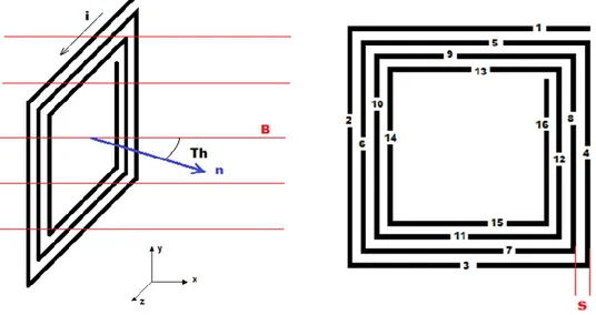
To study the magnetic dipole of a spiral coil it's easy to refer to a simple model considering spiral square coil in a magnetic field (Fig. 11). The problem is simplified assuming the B field and n normal to coil's surface on the same plane (Bn) that is perpendicular to the coil plane.
34
The Lorentz force on a single segment of wire is equal to:
⃗⃗⃗ ⃗
The analysis can be separated in 2 different part, firsts the segment parallel to the plane XZ (1,3,5,7,9,11,13,15) in y direction and then the segments perpendicular to the plane XZ (2,4,6,8,10,12,14,16) in z direction (Fig. 11).
Z direction:
The strength of each part of the coil parallel to the plane Bn gives a contribution that is alternately opposite in z direction. Part 1-5-9-13 would give a contribution that is in positive direction, while 3-7-11-15 will give a contribution in negative direction. Due to the fact that each piece is shorter than the previous one of a factor called s (wire diameter and space between two turns), the force at every turn will not be balanced by the following segment.
The sum of this contribution will provide a resultant force in positive direction of y equal to:
Y direction:
Repeating the same procedures for the vertical segment in z direction (2,4,6,8,10,12,14,16) it's possible to obtain the following forces in XZ plane:
35
Where the direction is alternating every time as the previous case.
In this case each segment will provide a torque to the coil that tends to align the normal direction n with the direction of the magnetic field B (Fig. 12).
Fig. 12 The torque (in yellow) tends to align the normal direction with the magnetic field
The arm of each force can be evaluated considering each segment and then calculate the torque. All the torques agree with the same sign.
( ) ( )
36
( ) ( ) ( ) ( )
Summing the torque with the same arm
[ ] ( ) [ ]
( ) [ ]
( ) [ ]
The total torque can be written as series
∑ [ ] ( )
Taking out the constant parameter from the series:
∑ [ ] ( )
Where it clearly appear the vector product:
⌊ ∑ [ ] ( )
37
Remembering the expression of the torque as cross product between m and B
⃗ ⃗⃗ ⃗ In this expression the magnetic dipole is equal to
⃗⃗ ∑ [ ] ( )
̂
The series substitutes the term nA that is not evaluable for a spiral because the number of turns and the area of each loop is indefinable. A solution could be to use a simplified model in which it is assumed as Area the average area between the inner loop and the outer loop and as number of turns the number obtained counting the tracks from the first going to the inner (Fig. 13).
Fig. 13 Schematization of square spiral for embedded coil analysis
38
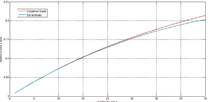
The difference in the results obtained with the two method gives the magnitude of the mistakes committed evaluating the magnetic dipole of the spiral coil with the simplified model (Fig. 14).
Fig. 14 Comparison between the simplified model and the spiral model
Assuming l=0.08 m and s=0.0005 the result show that for small number of turns the two model are pretty equivalent, while with the increase of the number of turns the overestimation made with the simplify model get more consistent. This is due to the fact that assuming a closed area for each loop it's an overestimation considering that no one loop is actually closed but is connected with the further. Increasing the number of turns increase also the error committed that could lead to a consecutive overestimation of the dipole moment.
The presence of a residual force parallel to the plane of the coil in up direction could consists in an attitude disturbance for the satellite
39
3.2.2 Balanced spiral in multilayer magnetorquer
Even if these residual forces are really low, these would tend to misalign the versor n with respect to the direction of B. But when this happens an arm for the torque would be created tending to realign n with B.
To compensate the residual force should be enough to reduce the starting
segment of quantity equal to 3s that represent the total amount not balanced (Fig. 11).
Would be therefore not possible to compensate at the same time also . The
solution to completely balance the magnetorquer could anyway to rotate the spiral in a multilayer embedded coil. Exploiting an even number of layer and alternating the position is possible to compensate the residual forces in pairs of two (Fig. 15).
40
3.2.3 Magnetic field strength
The magnetic field strength in the center of the spiral can be modeled to perform comparison with experimental results. The procedure is analogue to the one used to define the magnetic moment, exploiting the Biot Savart law for a wire crossed by a current I. ∫ ⃗⃗⃗
Taking in consideration the balanced spiral model each segment can be separated in two parts and the integral can be solved for each of these (Fig. 16).
Fig. 16 Square spiral scheme for H field analysis
The reason of the separation is to consider that at every spiral concentration the second half of the segment is reduced. We consider dB1.1 for the first half and dB1.2 for the second half.
41 ∫ ⃗⃗⃗ ∫ ⃗⃗⃗
Where l1.1 is the first half of l1 and l1.2 is the second half and so for the other segment.
Defining the relation for r and x:
∫
Solving the integral
|
√ |
Where h depends on the turns considered. Normally is possible to observe that 6 segment lead to the same results for every turns while the first and the last are different because of the spiral structure (Fig. 17).
42
Fig. 17 Square spiral scheme for H field analysis. Same colored segments give equal contribute
Also in this case it's possible to write a numerical series considering the space between parallel trace, the characteristic external dimensions and the spiral concentration (number of turns);
∑ { [ ]√[ ] [ ] [ ]√[ ] [ ] [ ]√[ ] [ ] }
Where Bn1 represents the contribution of the black segment and depends if the spiral is whether balanced or not. For a balanced spiral,
√ For a non-balanced spiral
43
√ Remembering the relation between H and B
It's possible to obtain the intensity of the magnetic field H simply eliminating the permeability from the previous expression.
The commonly used simplified model for a square spiral can be evaluated to define the mistakes committed in evaluating the H field with that approximation.
In case of a single square coil:
√ Simplifying the spiral with concentric square coils:
√
Where Lm is the medium side dimension between the outer and the inner turn. As for the magnetic moment, the two models differ more increasing the number of turns (Fig. 18).
44
Fig. 18 Comparison between simplified model and spiral model for the H field estimation
3.3 Designing issues
The modelled dipole permits to evaluate the better choice for the designing procedure of the embedded coil. In particular the parameter in which it's possible to operate the most are the copper trace width, the spiral concentration (that somehow represents the number of turns) and the number of layer.
As presented, the procedures will take in consideration the characteristic dimension as input parameter. In case of embedded coil this is absolutely logical solution considering that there would be no reason not to exploit at all the side surface of the satellite with the whole board. The number of layer can be used to determine the thickness of the board thinking a standard value for the insulation layer and the presence of top, bottom and ground layer.
Inputs:
Voltage supply
45
The copper cross sectional area influences the current reducing the resistance of the whole circuit. In general the thickness of the trace is a quite a standard value for a PCB that is 0.035 mm. However if necessary it can be possible to change also this parameter in the model to observe different results.
The parameter on which it's easy to act is the width of the trace during the designing phase. Several issues limit the possible value: thinner trace consists for a defined current to higher temperature increase of the circuit. Assuming a peak current no bigger than 1.5 A in the circuit and a temperature increase limited to 70° C for the circuit, the minimum value for the trace's width is set as 0.4 mm. In this case a nominal current under the level of 1.5 A will not over heat the board over the level of 70° C.
The power consumption can be evaluated calculating the length of the copper trace and the thickness of the layer to evaluate the total resistance of the coil.
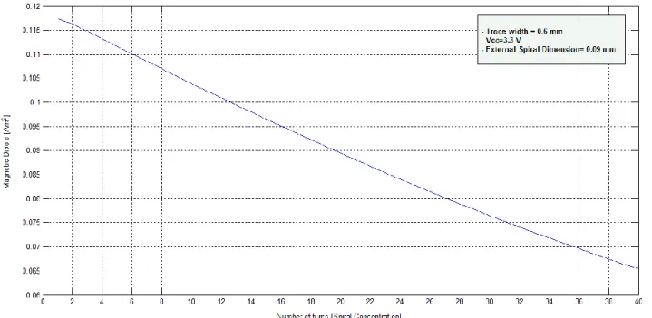
Assuming a defined voltage supply, the power consumption would decrease increasing the number of turns and in that way the total resistance of the trace. This consists in an increase of the trace length and concentration of the spiral, affecting the dipole in two opposite ways: the increase in the resistance reduces the current intensity but on the other side the product Area-number of turns is increased. The total effect would depend on the relation between the increase of Area-Turn product and the decrease of the current. Being the second linear with the number of turns and the first with a logarithmic growth, the general observed effect is a decrease of the dipole. This issue it's really important to understand that there is no advantage to densify the spiral on a layer to increase the dipole strength.
46
Fig. 19 Magnetic dipole reduction due to increase of spiral concentration
On the contrary the increase of the turns it's important to reduce the power consumption. If the required dipole is determined by a specific number of turns, the best way to reduce the power consumption maintaining that value is to increase the number of layers: this would consists in reproducing the same spiral trace in a parallel layer of the PCB (Fig. 20).
47
Fig. 20 Power consumption for a multilayer embedded coil
Nevertheless two big disadvantages are involved with this solution: first of all the mass of the PCB would consistently increase considering that any layer added requires a layer of insulation. Second, the cost of a multilayer board is many times higher than a single layer one.
The mass of the magnetorquer can be evaluated considering the mass of the copper layer and the mass of the insulating layer. This can be made in several materials even if FR4 is the most used and affordable. The reduction of copper layer could consist in a reduction of the total thickness of the board and in that way the mass. In spite of that, normally, the standard thickness of a 4 layer board is set at 1.6 mm with 0.035 mm copper thickness.
The mass can be evaluated considering the total mass of the copper trace and the mass of the needed insulator that has to be added when multilayer are required.
48
Fig. 21 Estimated mass increase for multilayer embedded coil
The mass increase can be observed in the graphs referred to the previous described case (Fig. 21).
The correct design for an embedded coil would be therefore to define the proper number of turns for a defined layer depending to the needed magnetic dipole and then increase the number of layer in order to reenter in the power budget constraints of the system. The general costs of this magnetorquer is pretty high compared to air core magnetorquer because the manufacturing of a multilayer PCB can cost many times more. The advantage of the embedded coil is the volume occupied and the easy integration in the satellite being embedded in the side panels. This is going to reduce the use of screw and other parts that add critical masses and risk during launch vibration.
3.4 Experimental measures on embedded coil
Several measures have been led on embedded coil magnetorquer to validate the model and to observe eventual issues not expected for this technology.
In this kind of magnetorquer the coil is "embedded" in a board composed by different material. This material could have a certain susceptibility to the magnetic field induced by the coil and they could affect it according to their magnetic
49
properties. In general it's possible to define 4 mean layer and parts that are standard for all embedded coil (Tab. 2):
Insulator layer
Ground plane
Solar Cell
Electronic Components
The insulator layer is the FR4 layer that is between two close copper coils. This is composed by fiber glass in epoxy resin. Glass is in general a diamagnetic material so the expected effect should be a reduction in the magnetic flux density. Though, the glass fibers are disposed on the plane and so perpendicular to the direction of the main applied field (perpendicular to the plane): the preferred direction of magnetic susceptibility should lie in the plane of the coil and in that way affect less the magnetic dipole.
The same concept can be applied to the ground plane that is composed by copper, even if in this case the diamagnetic properties of the material are really weak to determine a not negligible effect on the magnetic flux density.
The solar cell is the only element that could consistently interfere with the magnetic field generated by the coil. This because they are semiconductor material with high electron mobility and in that way high magnetic response. The different material which the solar cells are composed with can't allow to determine empirically a specific effect.
Material Relative Permeability
Magnetic Properties Ground plane Copper 0.999994 Diamagnetic
Insulator layer FiberGlass 0.999987 Diamagnetic
Solar Cell GaAs GaInP2 Ge ? ? Electronic Components Al, Si ? ?
50
Even if these materials have really small magnetic quantities individually, the simultaneous presence could lead to a chaining effect whose outcome is not predictable. This thinking also that electronic charging of different components under electronic field leads to magnetic effects.
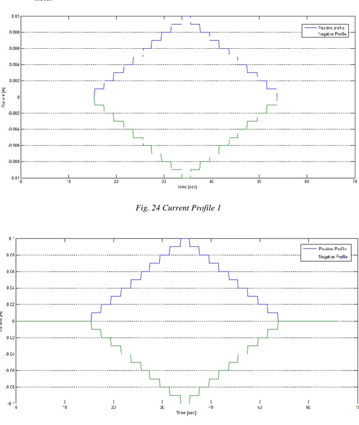
To evaluate the effect of the presence of different material in the complete board it has been performed an experimental measure. For the test have been studied two different boards with the same identical embedded magnetorquer, one with the mounted solar panel, and the other without. The two boards have been supplied with a defined profile current. The targets of the experiment were the following:
Determine the average permeability of the whole board and in that way understand the effect of layers of different material on the magnetic flux density.
Evaluate the difference between the mathematical model and the real case.
Investigate the presence of eventual residual magnetic field.
Evaluate the eventual interference of the solar panel on the magnetic flux density.
The experiment has been led exploiting the Helmholtz cage (Fig. 22,Fig. 23): with this device it's possible to compensate properly the earth magnetic field and generate a quasi-zero magnetic field in the measurement volume.
The Helmholtz cage needs to be calibrated before running every experiment. The calibration procedure has been made once the setup was complete and voltage generators turned on (providing zero current). In that way all the disturbance that couldn't be eliminated and could affect the following measures were kept into account in the calibration slope.