Synthesis of monopulse sub-arrayed linear and planar array antennas with optimized sidelobes

UNIVERSITY

OF TRENTO

DIPARTIMENTO DI INGEGNERIA E SCIENZA DELL’INFORMAZIONE 38123 Povo – Trento (Italy), Via Sommarive 14

http://www.disi.unitn.it

SYNTHESIS OFMONOPULSE SUB-ARRAYED LINEAR AND

PLANAR ARRAY ANTENNAS WITH OPTIMIZED SIDELOBES

G. Oliveri, L. Poli

January 2011

Synthesis of Monopulse Sub-arrayed Linear and Planar Array

Antennas with Optimized Sidelobes

G. Oliveri and L. Poli

ELEDIA Research Group

Department of Information Engineering and Computer Science, University of Trento, Via Sommarive 14, 38050 Trento - Italy Tel. +39 0461 882057, Fax +39 0461 882093

E-mail: {oliveri.giacomo, lorenzo.poli}@disi.unitn.it Web: http://www.eledia.ing.unitn.it

Synthesis of Monopulse Sub-arrayed Linear and Planar Array

Antennas with Optimized Sidelobes

G. Oliveri and L. Poli

Abstract

In this paper, three approaches for the synthesis of the optimal compromise between sum and difference patterns for sub-arrayed linear and planar arrays are presented. The synthesis problem is formulated as the definition of the sub-array configuration and the correspond-ing sub-array weights to minimize the maximum level of the sidelobes of the compromise difference pattern. In the first approach, the definition of the unknowns is carried out simul-taneously according to a global optimization schema. Differently, the other two approaches are based on a hybrid optimization procedures, exploiting the convexity of the problem with respect to the sub-array weights. In the numerical validation, representative results are shown to assess the effectiveness of the proposed approaches. Comparisons with previously published results are reported and discussed, as well.

Key words: Linear and Planar Arrays, Monopulse Antennas, Sum and Difference Patterns,

1

Introduction

Monopulse tracking radars [1] are based on the simultaneous comparison of sum and difference signals to compute the angle-error and to steer the antenna patterns in the direction of the tar-get (i.e., the boresight direction). Besides classical solutions where multi-feeder reflectors are considered, the two (sum and difference) or three (sum and double-difference) patterns, needed to determine the angular location of the target along a singular angular coordinate or both in azimuth and elevation, can be synthesized through linear or planar array antennas, respectively. Recent studies are mainly devoted to array solutions because of the larger number of degrees of freedom. As a matter of fact, such a solution allows one to control the illumination of the array directly on the aperture by modifying the excitations of the radiating elements. Moreover, the synthesized patterns are electronically steerable. This enables the fast change of the beam direction and it avoids the inertia problems due to the use of mechanical positioning systems. On the contrary, the drawbacks of the array implementation lay in the circuit complexity and the arising costs. Nevertheless, the elements of the aperture can be grouped into sub-arrays in order to simplify the antenna design and obtain cheaper tradeoff despite some reductions of the antenna performances [2][3].

In antenna systems applied for real world applications [4], different strategies for implementing monopulse radars have been adopted. A well known technique considers the partition of the array aperture into two halves (linear array) o four quadrants (planar arrays). The outputs of the elements belonging to the same half/quadrant are combined and continuously compared with the output/s of the other half/quadrants to determine the error signal. Such a signal is used to steer the sum and difference beams and thus to track the moving target.

In such a framework, recent papers have dealt with the optimal compromise problem between sum and difference patterns, starting from an optimum sum pattern generated by a complete and dedicated feed network. The elements of the array are then grouped into sub-arrays with a proper weighting to obtain a “sub-optimal” difference pattern. Either the optimization of some specific pattern features (e.g., the directivity [5][6][7], the normalized difference slope [8], the sidelobe level (SLL) [9][10]) or the fitting with an optimal pattern in the Dolph-Chebyshev

sense [11][12] have been considered. Among them, theSLL minimization of the compromise

different optimization strategies based on global optimization approaches [13][14] as well as two-step hybrid techniques [9][10][11][15] have been proposed. However, an effective and flexible procedure able to deal with both the synthesis of linear and planar structures has been previously proposed only in [9][12][16]. Such an event is mainly due to the exponential growth of the dimension of the solution space with the increase of the number of array elements. The approach proposed in [12] and then extended in [16], named Contiguous Partition Method (CP M), takes advantage from the knowledge of the relationship between the independent

dis-tributions of the optimal sum and difference [17] coefficients to reduce the dimension of the solution space. Accordingly, the synthesis of large planar arrays is enabled and the converge of the synthesis procedure speeded up. Essentially based on an excitation matching proce-dure, the sub-array configuration is first obtained by minimizing the distance between the refer-ence/optimal and synthesized (sub-arrayed) difference coefficients. Accordingly, the sub-array gains are directly computed as a function of the optimal sum and difference excitations exploit-ing the guidelines of [20]. Nevertheless, the CP M procedure does not allow to control the

level of the sidelobes. To overcome this drawback, preliminary results obtained by means of an iterative version of the CP M (the I − CP M) have been shown in [18] and [19]. There,

the optimal pattern to match is iteratively changed until the SLL of the compromise solution

satisfied the user-defined constraints.

In this paper, three new approaches aimed at the minimization of the SLL of the compromise

difference pattern are presented. In the first, the simultaneous optimization of the problem un-knowns is dealt with likewise [12], but in this case the so-called solution tree (i.e., the represen-tation of all the admissible sub-array configuration [12]) is explored looking the solution with minimumSLL. This strategy will be referred in the following as Modified CP M (M −CP M).

The other two approaches consider the hybridization of the I − CP M (HI − CP M) and of

theM − CP M (HM − CP M) with a Convex Programming (CP ) procedure [10] to directly

introduceSLL constraints in the optimization procedure.

The paper is organized as follows. In Sect. 2, the synthesis problem is mathematically formu-lated. The innovativeCP M-based procedure aimed at the optimization of the SLL is pointed

out in Sect. 3, where the one-step (Sect. 3.1) as well as the hybrid two-step (Sect. 3.2) are presented. A set of selected results concerning the synthesis of linear as well as planar arrays

is reported in Sect. 4 to assess the effectiveness of the proposed methods. Comparison with previously published results are also reported where available. Finally, some conclusions are drawn (Sect. 5).

2

Mathematical Formulation

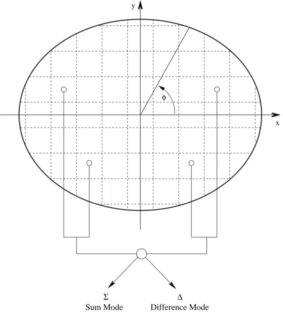
Let us consider either a linear or planar array with elements uniformly spaced in the xy-plane

(Fig. 1). The array factor is

f (u, v) = N

X

n=1

cnejk(uxn+vyn) (1)

wherecn,n = 1, ..., N, is the set of real excitations, u = sin θ cos φ and v = sin θ sin φ, where

the values (θ, φ), θ ∈h0,π 2

i

andφ ∈ [0, 2π] , indicate the angular direction, and k = 2π_λ is the wavenumber of the background medium. Moreover, (xn, yn) is the position of the n-th array

element.

To obtain sum and difference patterns, the distribution of the coefficients is supposed to be symmetric with respect to the physic center of the aperture. In particular and concerning the linear case, the two halves of the array are summed in phase and phase reversal, respectively. Differently, the aperture is supposed to be divided into four symmetric quadrants in the case of a planar array. Accordingly, the sum signal is obtained by adding in phase all the output of the four quadrants, while the difference modes, namely the azimuth difference mode (H − mode)

and the elevation difference mode (E − mode), are given with pair of quadrants added in phase

reversal.

The excitations of the “sub-optimal” difference pattern cn = dn, n = 1, ..., N, as obtained

through the sub-arrayed feed network are

dn =        PQ q=1snδanqwq −π/2 < φ ≤ π/2 PQ q=1(−1) snδanqwq π/2 < φ ≤ 3π/2 (2)

where S = {sn; n = 1, ..., N} is a set of fixed excitations affording an optimal sum pattern

[17], W = {wq; q = 1, ..., Q} are the (unknown) sub-array weights, A = {an; n = 1, ..., N}

is a integer vector where the element an ∈ [0, Q] indicating the sub-array membership (when an= 0 it follows that dn = sn) andδanqis the Kronecker delta (δanq = 1 if an= q and δanq = 0 otherwise). Since monopulse planar arrays require the generation of two spatially-orthogonal

difference patterns [4], the coefficients of the first difference mode are given as in (2), while the second difference mode is obtained by adding the two pairs of quadrants shifted by π/2 in the φ-direction with respect to (2).

Hence, the problem at hand is formulated as follows : “optimizing the sub-array configuration

Aoptand the corresponding set of weightsWoptto obtain a compromise difference pattern with minimum sidelobe level for a given main lobes beamwidth.”

3

Sidelobe Level Optimization Approaches

In this section, three new approaches for the solution of the optimal compromise between sum and difference patterns are described, where the SLL optimization of the difference beams is

dealt with. In particular, the simultaneous optimization of both the sub-array aggregation and the sub-array gains is firstly considered according to theM − CP M (Sect. 3.1) and the main

differences with respect to theI − CP M [18] are pointed out. Then, their hybridized two-step

versions, namely theHI − CP M and the HM − CP M are presented in Sect. 3.2, as well.

3.1

Simultaneous Definition of the Unknowns

As far as the simultaneous synthesis of the problem unknowns is concerned, the Iterative

Con-tiguous Partition Method (I − CP M) has been successfully applied. Its procedure and some

preliminary results have been already published in [18] and [19], where linear and planar array synthesis problems have been dealt with, respectively. In particular, theI − CP M is based on

the following concept: by successively changing the reference/optimal target to approximate, at each step the CP M [12] is applied until the requirements on the SLL for the synthesized

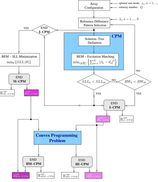
difference pattern are satisfied. It is worth to notice that in theI − CP M [19], whose workflow

is schematically outlined in Fig. 2, the optimization of theSLL is obtained as a by-product. As

a matter of fact, the bare version of the CP M [12] concerns the definition of the “best

com-promise” difference pattern close as much as possible to the optimal one through an excitation matching procedure. Nevertheless, enforcing the CP M to iteratively approximate an optimal

difference pattern with a reference SLL lower and lower, it allows to reduce the SLL of the

The strategy proposed in this work, namely the Modified Contiguous Partition Method (M − CP M), tries to to explore the solution tree [12], directly looking for the solution with minimum SLL, unlike the one guaranteeing the best least-square pattern matching. The solution with the

lowest SLL is searched by means of the border element method (BEM) described in [12].

Towards this aim, the following cost function is considered

ΨM−CP M(A, W ) = min

u,v {SLL (u, v)} (3)

for the linear and planar case, whereSLL (u, v) is the maximum level of the sidelobes outside

the main lobe region. Let us we refer to this procedure as the .

It is worth noting that both theI − CP M and the M − CP M allow the simultaneous definition

of all the problem unknowns in a reliable and efficient way since the are based on the CP M.

As a matter of fact, whether on one hand the final sub-array aggregation is obtained through the

BEM, which computational efficiency has been pointed out in [2], on the other hand the

defi-nition of the sub-array weights does not increase the computational burden, since an analytical relationship [12] is considered: wqCP M = " PN n=1δanq(snβn) PN n=1δanq(sn) 2 # ; q = 1, ..., Q (4)

whereB = {βn; n = 1, ..., N} is the set of optimal difference excitations [17].

3.2

Two-Step Hybrid Approaches

Inspired by the investigations on the synthesis of difference patterns carried out in [21], it has been recently discussed in [10] how the definition of the sub-array weights can be formulated as the solution of a convex programming problem, once the clustering of the array elements is given. However, in [10] the solution of a the CP problem is required every time a new

sub-array configuration is obtained by means of the an approach based on Simulated Annealing (SA). Therefore, the SA − CP approach turns out to be affected by an unavoidably and high

computational cost.

In order to cope with this drawback, in the following two new hybrid (two-step) approaches are proposed, where the solution of the CP problem is required only once during the whole

synthesis process. The flowchart of both the approaches is schematically depicted in Fig. 2. More specifically, at the first step the sub-array configurations are computed according to the principles of either theM − CP M or the I − CP M [18]. Successively, the sub-array weights, Wopt ₌n

w(opt)

q ; q = 1, ..., Q

o

, of the compromise feed network are computed so that theSLL

of the afforded pattern is below a pre-fixed threshold. The following cost function

ΨCP (W ) = ∂Re {f (u, v)} ∂u∂v      u = u 0 v = v0 (5)

is minimized subject to ∂Im{f (u,v)}_∂u∂v  

u = u0 v = v0

= 0, to f (u0, v0) = 0 and a function descriptive of

an upper maskUB (u, v) on the synthesized difference pattern. Moreover, Re and Im denotes

the real and imaginary part, respectively and (u0, v0) is the boresight direction. Towards this

end, a standardCP procedure is used, whose initial guess solution is given by W(0)as computed through Eq. (4).

4

Numerical Simulations and Results

In order to show the effectiveness and the versatility of the proposed approaches, different syn-thesis problems concerning linear (small and large) as well as planar monopulse array antennas are shown in this section. In order to better point out the advantages and limitations of the si-multaneous/global optimization and of the hybrid procedures, the numerical analysis has been subdivided in two parts. The first one (Sect. 4.1) concerns with the syntheses of small linear arrays, where the total number of unknowns is small (N ≤ 20) and both global and hybrid

approaches reach the final solution in a limited amount of time (i.e., in the order of one minute or less). The capability to deal with large linear arrays and planar apertures, characterized by a large number of radiating elements, is then considered in Sect. 4.2. Comparisons with bench-marks already reported in the literature are considered where available.

4.1

Small Linear Arrays Synthesis

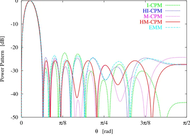
In the first test, let us consider a linear array of N = 20 elements equally spaced of λ/2. The

sum excitations are chosen to afford a Villeneuve pattern with SLL = −25 dB and n = 4

[22]. The number of sub-arrays has been set equal to Q = 5. In this case the results obtained

by means of the proposed approaches are compared with the pattern synthesized by means of the constrained Excitation Matching Method (EMM) of [11], where the final pattern was

characterized bySLL = −23.4 dB.

As far as the proposed approaches are concerned, the optimal difference excitation set consid-ered in theM − CP M is chosen to correspond to the one used at the last step of the I − CP M.

Moreover, since the constrainedEMM [11] is also an excitation matching procedure, we force

theI − CP M to avoid a reference target with SLL lower than that considered in [11] (i.e., a

modified Zolotarev difference pattern withSLL = −25 dB, n = 4 and ǫ = 3 [23]).

The sub-array configurationsAopt_{I−CP M}, Aopt_{M−CP M} as well as the corresponding sub-array gains

Wopt_{I−CP M},Wopt_{M−CP M} obtained at the final iterations by the two global optimization techniques are summarized in Tab. I. The corresponding patterns are shown in Fig. 3. As expected, improvements in term ofSLL minimization are given by the M −CP M with a SLL lowered of

almost2 dB (i.e., SLLI−CP M = −22.4 dB vs. SLLM−CP M = −24.3 dB). In this experiment,

only the M − CP M outperforms the EMM in terms of SLL minimization. As far as the

computational burden is concerned, thanks to the computational efficiency of the BEM [12]

and by virtue of the fact that the sub-array weights are computed analytically, the required

CP U time is equal to TI−CP M = 0.05 sec and TM−CP M = 0.24 sec, while kI−CP M = 19 and kM−CP M = 4 is the total number of cost function evaluations.

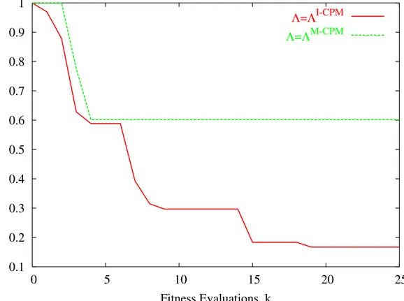
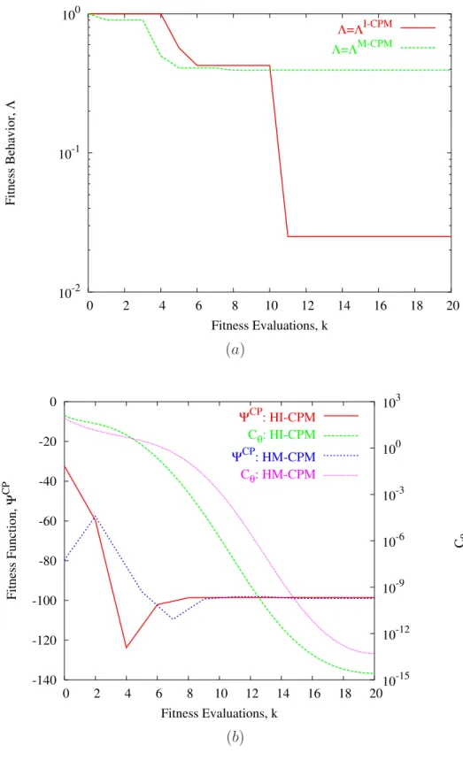
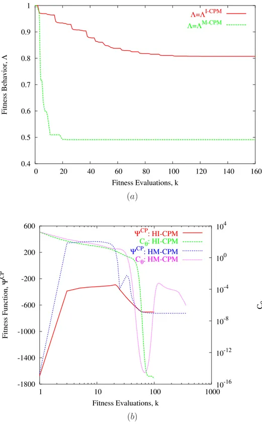
In order to complete the analysis, Fig. 4 reports the values of the cost function of theI − CP M

as well as that of the M − CP M. Since two incommensurable quantities are minimized, in

order to make the comparison meaningful the following relationship has been considered for the plots of the fitness

Λ = 1 − |ξk− ξ max_|

|ξmax_| , k = 1, ..., K (6)

where ξk assumes either the valueΨM−CP Mk (3) orΨ I−CP M

k [18], according to the use of the M − CP M or I − CP M, respectively. Moreover, ξmax _{= max}

i=1,...,K{ξi} is the maximum

As a second step, the final aggregations obtained by means of the bare approaches (Tab. I) are considered as fixed clustering in the H − ICP M and H − MCP M, i.e., Aopt_{H−ICP M} = Aopt_{ICP M} andAopt_{H−M CP M} = Aopt_{M CP M}, respectively. Then, the sub-array weights are determined through the subroutine FMINCON [24], where the mask UB (θ) has been set to have BW = BWEM M and uniform level of sidelobes. Accordingly, starting from a guess solution equal

to W(0)H−ICP M = W opt ICP M and W (0) H−M CP M = W opt

M CP M, the weights of the sub-arrays are

computed by the two hybrid approaches and the corresponding results are reported in Tab. I . Also in this case, the synthesized patterns are shown in Fig. 3. It is worth noting that both the solutions achieved by the hybrid approaches have aSLL below the one obtained with the EMM [11], i.e., SLLHI−CP M = −24.4 dB, SLLHM−CP M = −25.8 dB vs. SLLEM M = −23.4 dB. Moreover, the hybrid versions are more effective in term of SLL minimization than

the respective bare procedures, with an improvement of 2 dB and 1 dB for the HI − CP M

andHM − CP M, respectively. As a matter of fact, notwithstanding the CP problem is aimed

at the maximization of the difference slope, the same hybrid approaches can be used for the optimization of theSLL, as pointed out in [10].

Fig. 5 reports the valuesΨCP

k ,k = 1, ..., K (k being the iteration index) as well as the maximum

distanceCθ between the actual pattern and the mask Cθ

k = maxθ{fk(θ) − UB (θ)} −π₂ ≤ θ ≤ π₂ (7)

wherefk(θ) is the array factor of the trail solution at the k-th iteration. As far as the costs of

the subroutine FMINCON [24] are concerned, let us first point out that the number of function evaluations to reach the final solutions is equal to kH−ICP M = 1001 and kH−M CP M = 83.

The overallCP U-time required to obtain WoptH−ICP M andW opt

H−M CP M amounts toTH−ICP M = 61.22 sec and TH−M CP M = 9.66 sec, with a non-negligible cost saving of almost six times for

theHM − CP M against the HI − CP M.

As a second experiment, let us consider one of the benchmark of [10], previously proposed in [14]. The number of sub-array was set to Q = 6 and the sum excitations fixed to those

of a Dolph-Chebyshev pattern withSLL = −20 dB [25], while the difference excitations are

those of a Zolotarev pattern with SLL = −31 dB [26]. Similarly to the previous case, the

synthesis problems consists in defining the sub-array clustering and weights in order to obtain a compromise difference beam with the lowestSLL, once the pattern beamwidth has been fixed

to that obtained by Differential Evolution (DE) optimization in [14].

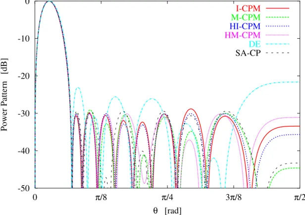
The sub-array configuration achieved in [10] in the case ofSLL optimization was Aopt_SA−CP = [1 5 2 3 3 4 2 5 6 1 1 6 5 2 4 3 3 2 5 1] with a maximum SLL = −30 dB. For the sake of

compari-son, the result achieved by theSA−CP in the case of maximization of the slope (where a value SLL = −29.50 dB was reached) has been reported in Fig. 6 as well as the one obtained with

theDE-based approach [14], together with those synthesized through the proposed approaches.

Concerning the two globalCP M-based approaches, the I − CP M and the M − CP M achieve

two different sub-array configurations, namely Aopt_{I−CP M} = [2 4 5 6 6 6 5 4 3 1 1 3 4 5 6 6 6 5 4 2]

andAoptM−CP M = [1 3 4 5 6 6 4 3 2 1 1 2 3 4 6 6 5 4 3 1], among the 126 solutions defined in the

so-lution tree [12]. The corresponding sub-array weights turns out beingWopt_{I−CP M} = {0.1641, 0.2422, 0.4652, 0.6917

and Wopt_{M−CP M} = {0.2081, 0.4652, 0.6917, 0.8776, 0.9840, 1.0044}. Moreover, TI−CP M =

0.001 sec, TM−CP M = 0.267 sec and kI−CP M = 12, kM−CP M = 10. Also the solutions

achieved by the hybrid versions are shown in Fig. 6. In these cases, kHI−CP M = 15 and

kHM−CP M = 16 function evaluations were needed with a required CP U time of THI−CP M =

2.703 sec and THM−CP M = 2.719 sec. The corresponding sub-array weights are WoptHI−CP M =

{0.6676, 0.9174, 1.7668, 2.6966, 3.4241, 3.8810} and WoptHM−CP M = {0.8019, 1.8409, 2.6401, 3.5552, 3.7342

It is interesting to note how all the solutions defined by means of the proposed approaches outperform that of [14], whereas only the solutions obtained by means of hybrid approaches

HI − CP M and HM − CP M are able to enhance the performances of [10]. As a matter of

factSLLI−CP M = −28.81 dB , SLLM−CP M = −29.12 dB, SLLHI−CP M = −30.09 dB and

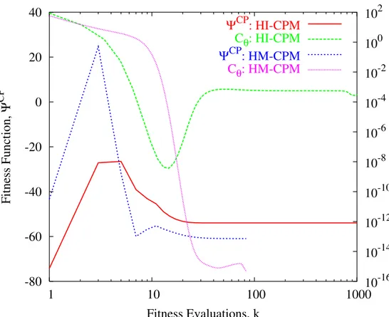
SLLM I−CP M = −30.13 dB. In order to complete the analysis, the behavior of the objective

functions for the global optimization procedures as well as their hybrid versions are reported in Fig. 7(a) and Fig. 7(b), respectively.

4.2

Large Linear Arrays and Planar Apertures

This section is aimed at analyzing the performances of the proposed approaches when dealing with the synthesis of array with a large number of elements. In the first example a linear aperture of length100λ is considered, whit N = 200 elements equi-spaced of λ

2. The sum excitations are

fixed to afford a Dolph-Chebyshev pattern [25] withSLL = −25 dB. The number of available

known trade-off exists between pattern beamwidth andSLL, the I − CP M is not allowed to

use reference targets whose SLL is below the one taken into account in [12] (i.e., a Zolotarev

difference pattern [26] withSLL = −30 dB). Fig. 8 shows the compromise difference patterns

synthesized by means of the proposed procedures. As expected, the solution obtained with the

I − CP M is the same obtained with the CP M [12]. The behavior of the fitness values for the

global and hybrid approaches are shown in Fig. 9(a) and Fig. 9(b), respectively.

Although all the solutions show a good behavior in term of sidelobes rejection, theHM −CP M

outperformed the other approaches with SLLHM−CP M = −27.1 dB, while SLLI−CP M = −25.2 dB, SLLM−CP M = −26.2 dB and SLLHI−CP M = −26.5 dB. The sub-array

configu-rations as well as the corresponding sub-array weights are given in Tab. II.

Concerning the computational costs, the number of cost function evaluation and the required

CP U time for each approach are reported in Tab. III. It is worth noting that in this case the

computational burden of the CP problem is non-negligible (i.e., THI−CP M = 4105.12 and THM−CP M = 957.51 sec). Such a drawback is principally due to the computation of Cθ, where

the pattern has to be sampled densely in order to obtain satisfactory results. Likewise, the computation of the power pattern is necessary also in theM − CP M to evaluate the SLL for

each trial solution. Therefore, theI − CP M [18] turns out to be in this case the most efficient

strategy.

In the last example, in order to fully exploit the capabilities of theCP M-based approaches, let

us consider a planar array with circular boundary r = 4.85 λ and N = 300 elements

equally-spaced of d = λ

2 along the two coordinates. The sum mode is set to a circular Taylor pattern

[27] withSLL = −35 dB and n = 6 . Moreover, Q = 3 sub-arrays have been considered. The

synthesis problem has been originally dealt with in [9] by means of a SA-based algorithm and

then considered as benchmark in [19][16]. There, the sidelobe ratio (SLR) defined as

SLR (φ) = SLL (φ)

maxθ[f (θ, φ)]

, 0 ≤ θ < π

2 (8)

was optimized. Unlike [19], in this case we are aimed at synthesizing a compromise difference pattern with aSLL low as much as possible. As far as the I −CP M is concerned, the reference

excitations (at the last iteration) was set in [19] to those a Bayliss pattern [28] with SLL = −35 dB and n = 6. In this case, the SLL was equal to the one obtained with the SA-based

was expected by using its hybrid version, in this case the achieved compromise configuration affords a pattern with SLLHI−CP M = −18.9 dB, worse than the one obtained with the I − CP M. On the contrary, the M −CP M synthesized a solution with SLLM−CP M = −24.45 dB,

almost than5 dB below the solution of [9]. Moreover, an additional improvement of more than 2 dB was gained when using the HM − CP M (i.e., SLLM−CP M = −26.55 dB).

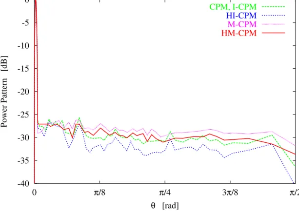
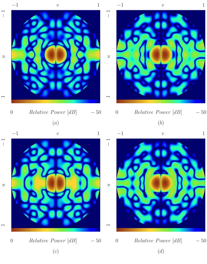
Fig. 10 show the 2D plots of the relative power patterns for all the compromise solutions. The corresponding sub-array configurations are shown in Fig. 11, while the sub-array weights for the four approaches are summarized in Tab. IV. Although the proposed approaches are aimed the optimization of the maximumSLL on the whole aperture, in this case both M − CP M and HM − CP M guaranteed that also the values of SLR were lower than that of [9] (Fig. 12).

Concerning the computational costs, it turns out that THI−CP M = 24186.6 sec (almost seven

hours) and THM−CP M = 39036.8 sec (more than ten hours). Moreover, kHI−CP M = 6621 and kHM−CP M = 10001. On the contrary, the computational cost reduces to TM−CP M = 537.9 sec, TI−CP M = 165.5 sec, and kM−CP M = 6, kI−CP M = 81 for the bare approaches.

5

Conclusions

In this paper, innovative approaches to the synthesis of the optimal compromise between sum and difference patterns for sub-arrayed monopulse array antennas have been presented. The synthesis of linear and planar array has been deal with, where the problem at hand has been formulated as the definition of the sub-array configuration and weights of these latter to min-imize the SLL of the synthesized difference beam. The definition of the unknowns has been

simultaneously carried out according to a global optimization schema, theM − CP M, and the

results have been compared with the previously proposed I − CP M. Unlike the I − CP M,

the compromise solution with minimumSLL has been directly looked for among the solutions

belonging to the solution tree. In a different fashion, theHI − CP M and the HM − CP M

have shown better performance in term ofSLL minimization with respect to the corresponding

one-step approaches. In these case, the convexity of the problem with respect to a part of the unknowns has been exploiting, where the synthesis problem has been reduced to solve a CP

problem for a fixed clustering. The effectiveness of the proposed techniques in terms of SLL

large array synthesis problems, hardly to manage with stochastic optimization procedures for the arising computational burden. Moreover, by virtue of the fact that the solution of the CP

problem is required only once, the hybridCP M-based strategies seem to represent promising

References

[1] I. M. Skolnik, Radar Handbook. McGraw-Hill, 1990.

[2] P. Rocca, L. Manica, A. Martini, and A. Massa, “Synthesis of large monopulse linear ar-rays through a tree-based optimal excitations matching,” IEEE Antennas Wireless Propag.

Lett., vol. 6, pp. 436-439, 2007.

[3] L. Manica, P. Rocca, and A. Massa, “On the synthesis of sub-arrayed planar array antennas for tracking radar applications,” IEEE Antennas Wireless Propag. Lett., vol. 7, pp. 599-602, 2008.

[4] S. M. Sherman, Monopulse Principles and Techniques. Artech House, 1984.

[5] A. Massa, M. Pastorino, and A. Randazzo, A., “Optimization of the directivity of a monopulse antenna with a subarray weighting by a hybrid differential evolution method,”

IEEE Antennas Wireless Propagat. Lett., vol. 5, pp. 155-158, 2006.

[6] P. Rocca, L. Manica, and A. Massa, “Directivity optimization in planar sub-arrayed monopulse antenna,” Progress in Electromagnetic Research L, vol. 4, pp. 1-7, 2008. [7] L. Manica, P. Rocca, and A. Massa, “An excitation matching procedure for sub-arrayed

monopulse arrays with maximum directivity,” IET Radar, Sonar & Navigation, vol. 3, no. 1, pp. 42-48, 2009.

[8] L. Manica, P. Rocca, M. Pastorino, and A. Massa, “Boresight slope optimization of sub-arrayed linear arrays through the contiguous partition method,” IEEE Antennas Wireless

Propag. Lett., vol. 8, pp. 253-257, 2008.

[9] F. Ares, S. R. Rengarajan, J. A. Rodriguez, and E. Moreno, “Optimal compromise among sum and difference patterns through sub-arraying,” Proc. IEEE Antennas Propagat. Symp., pp. 1142-1145, 1996.

[10] M. D’Urso, T. Isernia, and E. T. Meliadò, “An effective hybrid approach for the optimal synthesis of monopulse antennas, ” IEEE Trans. Antennas Propag., vol. 55, no. 4, pp. 1059-1066, Apr. 2007.

[11] D. A. McNamara, “Synthesis of sub-arrayed monopulse linear arrays through matching of independently optimum sum and difference excitations,” IEE Proc. H Microwaves

Anten-nas Propag., vol. 135, no. 5, pp. 371-374, 1988.

[12] L. Manica, P. Rocca, A. Martini, and A. Massa, “An innovative approach based on a tree-searching algorithm for the optimal matching of independently optimum sum and difference excitations,” IEEE Trans. Antennas Propag., vol. 56, no. 1, pp. 58-66, Jan. 2008.

[13] P. Lopez, J. A. Rodriguez, F. Ares, and E. Moreno, “Subarray weighting for difference pat-terns of monopulse antennas: joint optimization of subarray configurations and weights,”

IEEE Trans. Antennas Propag., vol. 49, no. 11, pp. 1606-1608, 2001.

[14] S. Caorsi, A. Massa, M. Pastorino, and A. Randazzo, “Optimization of the difference patterns for monopulse antennas by a hybrid real/integer-coded differential evolution method,” IEEE Trans. Antennas Propag., vol. 53, no. 1, pp. 372-376, 2005.

[15] P. Rocca, L. Manica, R. Azaro, and A. Massa, “A hybrid approach to the synthesis of subarrayed monopulse linear arrays,” IEEE Trans. Antennas Propag., vol. 57, no. 1, pp. 280-283, Jan. 2009.

[16] L. Manica, P. Rocca, M. Benedetti, and A. Massa, “A fast graph-searching algorithm enabling the efficient synthesis of sub-arrayed planar monopulse antennas,” IEEE Trans.

Antennas Propag., vol. 57, no. 3, pp. 652-663, Mar. 2009.

[17] R. S. Elliott, Antenna Theory and Design. Wiley-Interscience IEEE Press, 2003.

[18] P. Rocca, L. Manica, A. Martini, and A. Massa, “Design of compromise sum-difference patterns through the iterative contiguous partition method,” IET Microw. Antennas

Propag., vol. 3, no. 2, pp. 348-361, 2009.

[19] P. Rocca, L. Manica, and A. Massa, “An effective excitation matching method for the synthesis of optimal compromises between sum and difference patterns in planar arrays,”

[20] W. D. Fisher, “On grouping for maximum homogeneity,” American Statistical Journal, pp. 789-798, 1958.

[21] O. Bucci, M. D’Urso, and T. Isernia, “Optimal synthesis of difference patterns subject to arbitrary sidelobe bounds by using arbitrary array antennas,” IEE Proc. Microwaves

Antennas Propag., vol. 152, no. 3, pp. 129-137, Jun. 2005.

[22] A. T. Villeneuve, “Taylor patterns for discrete arrays,” IEEE Trans. Antennas Propag., vol. 32, pp. 1089-1093, 1984.

[23] D. A. McNamara, “Performance of Zolotarev and modified-Zolotarev difference pattern array distributions,” IEE Proc. Microwave Antennas Propag., vol. 141, no. 1, pp. 37-44, 1994.

[24] T. Coleman, M. A. Branch, and A. Grace, Optimization toolbox user’s guide - for use with

Matlab. Natick: The Mathworks, Inc., 1999.

[25] C. L. Dolph, “A current distribution for broadside arrays which optimises the relationship between beam width and sidelobe level,” IRE Proc., vol. 34, pp. 335-348, 1946.

[26] D. A. McNamara, “Direct synthesis of optimum difference patterns for discrete linear arrays using Zolotarev distribution,” IEE Proc. H Microwave Antennas Propag., vol. 140, no. 6, pp. 445-450, 1993.

[27] T. T. Taylor, “Design of a circular aperture for narrow beamwidth and low sidelobes,”

Trans. IRE Antennas Propag., vol. 8, pp. 17-22, 1960.

[28] E. T. Bayliss, “Design of monopulse antenna difference patterns with low sidelobes,” Bell

FIGURE CAPTIONS

• Figure 1. Planar array geometry.

• Figure 2. Pictorial representation of the CPM-based approaches. • Figure 3. Small Linear Array (N = 20, d = λ

2,Q = 5) - Relative power patterns obtained

by means of the proposed approaches and theEMM [11]. • Figure 4. Small Linear Array (N = 20, d = λ

2,Q = 5) - Behavior of the cost function of

theI − CP M and M − CP M versus the iteration index k. • Figure 5. Small Linear Array (N = 20, d = λ

2, Q = 5) - Behavior of the cost function

and evolution of the distance from the constraints for theHI − CP M and HM − CP M

versus the iteration indexk.

• Figure 6. Small Linear Array (N = 20, d = λ₂,Q = 6) - Relative power patterns obtained

by means of the proposed approaches, theSA − CP [10] and the DE [14]. • Figure 7. Small Linear Array (N = 20, d = λ

2,Q = 6) - Behavior of the cost function of

the (a)I − CP M and M − CP M and of the (b) HI − CP M and HM − CP M versus

the iteration indexk.

• Figure 8. Large Linear Array (N = 200, d = λ

2, Q = 6) - Relative power patterns

obtained by means of the proposed approaches and theCP M [12]. • Figure 9. Large Linear Array (N = 200, d = λ

2, Q = 6) - Behavior of the cost function

of the (a)I − CP M and M − CP M and of the (b) HI − CP M and HM − CP M versus

the iteration indexk.

• Figure 10. Planar Array Synthesis (N = 300, d = λ

2, r = 4.85λ, Q = 3) - Relative

power patterns obtained by means of (a) the I − CP M, (b) the M − CP M, (c) the HI − CP M and (d) HM − CP M.

• Figure 11. Planar Array Synthesis (N = 300, d = λ₂, r = 4.85λ, Q = 3) - Sub-array

• Figure 12. Planar Array Synthesis (N = 300, d = λ

2, r = 4.85λ, Q = 3) - Plots of

the synthesizedSLR values by means of the proposed approaches and the SA [9] in the

TABLE CAPTIONS

• Table I. Small Linear Array (N = 20, d = λ

2, Q = 5) - Sub-array configurations and

weights.

• Table II. Large Linear Array (N = 200, d = λ

2, Q = 6) - Sub-array configurations and

weights.

• Table III. Large Linear Array (N = 200, d = λ

2,Q = 6) - Fitness evaluations and CP U

time.

• Table IV. Planar Array Synthesis (N = 300, d = λ

2, r = 4.85λ, Q = 3) - Sub-array

φ

y

x

Σ ∆

Sum Mode Difference Mode

BEM − Excitation Matching Solution−Tree Definition Pattern Selection Reference Difference Configuration NO NO CPM BEM − SLL Minimization YES YES Problem YES Array subarray number: optimal sum mode:

Convex Programming END I−CPM END M−CPM I−CPM END END HI−CPM END HM−CPM min(A,W ) n PN n=1|βn− dn|2 o SLLk< SLLth BWk< BWth minθ{SLL (θ)} Wopt_{I−CP M} Wopt_{HI−CP M} Wopt_{HM −CP M} Wopt_{M −CP M} Aopt_{M −CP M} Aopt_{HM −CP M} Aopt_{I−CP M} Aopt_{HI−CP M} Q sn, n = 1, ..., N βn, n = 1, ..., N

-50 -40 -30 -20 -10 0 0 π/8 π/4 3π/8 π/2 Power Pattern [dB] θ [rad] I-CPM HI-CPM M-CPM HM-CPM EMM

0.1 0.2 0.3 0.4 0.5 0.6 0.7 0.8 0.9 1 0 5 10 15 20 25 Fitness Behavior, Λ Fitness Evaluations, k Λ=ΛI-CPM Λ=ΛM-CPM

-80 -60 -40 -20 0 20 40 1 10 100 100010 -16 10-14 10-12 10-10 10-8 10-6 10-4 10-2 100 102 Fitness Function, Ψ CP Cθ Fitness Evaluations, k ΨCP : HI-CPM C_θ: HI-CPM ΨCP : HM-CPM C_θ: HM-CPM

-50 -40 -30 -20 -10 0 0 π/8 π/4 3π/8 π/2 Power Pattern [dB] θ [rad] I-CPM M-CPM HI-CPM HM-CPM DE SA-CP

10-2 10-1 100 0 2 4 6 8 10 12 14 16 18 20 Fitness Behavior, Λ Fitness Evaluations, k Λ=ΛI-CPM Λ=ΛM-CPM (a) -140 -120 -100 -80 -60 -40 -20 0 0 2 4 6 8 10 12 14 16 18 2010 -15 10-12 10-9 10-6 10-3 100 103 Fitness Function, Ψ CP Cθ Fitness Evaluations, k ΨCP : HI-CPM C_θ: HI-CPM ΨCP : HM-CPM C_θ: HM-CPM (b)

-40 -35 -30 -25 -20 -15 -10 -5 0 0 π/8 π/4 3π/8 π/2 Power Pattern [dB] θ [rad] CPM, I-CPM HI-CPM M-CPM HM-CPM

0.4 0.5 0.6 0.7 0.8 0.9 1 0 20 40 60 80 100 120 140 160 Fitness Behavior, Λ Fitness Evaluations, k Λ=ΛI-CPM Λ=ΛM-CPM (a) -1800 -1400 -1000 -600 -200 200 600 1 10 100 100010 -16 10-12 10-8 10-4 100 104 Fitness Function, Ψ CP Cθ Fitness Evaluations, k ΨCP : HI-CPM C_θ: HI-CPM ΨCP : HM-CPM C_θ: HM-CPM (b)

−1 v 1 −1 v 1 1 u − 1 1 u − 1

0 Relative P ower [dB] − 50 0 Relative P ower [dB] − 50

(a) (b) −1 v 1 −1 v 1 1 u − 1 1 u − 1

0 Relative P ower [dB] − 50 0 Relative P ower [dB] − 50

(c) (d)

LEGEND: 1st subarray 2nd subarray 3rd subarray (a) LEGEND: 1st subarray 2nd subarray 3rd subarray (b)

-35 -30 -25 -20 -15 -10 0 10 20 30 40 50 60 70 80 SLR [dB] φ [deg] I-CPM HI-CPM M-CPM HM-CPM SA

N = 20

A

, A

3 4 5 5 5 4 3 3 2 1 1 2 3 3 4 5 5 5 4 3

A

, A

3 4 5 5 5 4 4 3 2 1 1 2 3 4 4 5 5 5 4 3

Q = 5

W

0.1738 0.5083 0.9561 1.3299 1.4775

W

0.1738 0.5083 0.8358 1.2042 1.4775

W

0.2896 0.7476 1.4378 2.1858 2.3207

W

0.3423 0.7816 1.6012 2.1233 2.7166

M = 100 aI−CP M_n , n = 1, ..., M 1111111111111122222222333333334444444455555555566666666666666666666666666666666555555555444444433331 aM_n −CP M, n = 1, ..., M 1111111112222222333333333333334444444444555555555555666666666666666666666655555555555444444444443332 Q = 6 WI−CP M _{0.8206 1.4472 2.0200 2.5000 2.9000} WM−CP M _{0.3739 1.0060 1.8017 2.5520 3.0300} WHI−CP M _{0.2132 0.7236 0.9411 1.0909 1.2754} WHM−CP M 0.1134 0.3327 0.6773 1.1001 1.1871 T a b . II -G . O liv er i et a l., “S y n th es is o f M o n o p u ls e ...” 3 4

Approach

k

T [sec]

I − CP M

128

15.6

HI − CP M

383 4105.17

M − CP M

24

519.98

HM − CP M

95

957.51

Approach

w

w

w

I − CP M

0.3499 0.9333 1.4170

M − CP M

0.2870 0.8120 1.3886

HI − CP M

0.3684 2.4088 4.0573

HM − CP M

0.3313 0.9719 1.4113

SA [9]

1.69

3.69

5.00