ROBUST REGRESSION TREES BASED ON M-ESTIMATORS G. Galimberti, M. Pillati, G. Soffritti
1. INTRODUCTION
Although robust methods have a long history, only in the last four decades has the field of robust statistics experienced substantial growth as a research area. The demand for such methods has been driven by the increasing availability of com-plex and large data sets, in which atypical observations may be present. While ro-bust methods are well-established for studying data sets under univariate models, this is not the case for more complicated multivariate situations.
As far as regression problems are concerned, the interest is in modelling the re-lationship between a dependent variable Y and a p-dimensional vector of predic-tors (X1, ...Xj..., Xp) , with p≥1, as follows:
1
( ,... ..., ) 1, ,
i i ij ip i
Y = f x x x +u i = … , (1) n
where f (⋅) is an unknown function, Yi represents the dependent variable for
a generic unit, xij is the i-th observation of the j-th predictor and ui denotes a
random variable representing the error term corresponding to the i-th observa-tion.
A simple and well-known regression model is the linear one (see for example Montgomery et al., 2006). In this model, it is assumed that f (⋅) is a parametric lin-ear function. Furthermore, under the assumption of normality, ui, i = 1, ... , n are
i.i.d. N(0, σ2). The most frequently-used estimation technique for this model is ordinary least squares (LS), in which the unknown parameters have to be esti-mated by those functions of the sample observations that minimize the sum of the squared residuals. However, it is well-known from the parametric regression theory that the estimates of the unknown function f (⋅) based on such a criterion can perform poorly when the distribution of the error terms is not normal, par-ticularly in case of heavy-tailed distribution.
This problem has been addressed using two different approaches. The first consists of identifying influential observations and removing them from the sam-ple before estimating the model parameters. The identification of such observa-tions is generally performed through some regression diagnostics aiming at
meas-uring the leverage and influence of each sample observation. Some well-known and widely-used diagnostics are described, for example, in Rousseeuw and Leroy (1987) and Montgomery et al. (2006). A more recent solution within this ap-proach, also known as the forward search, is based on a suitable combination of re-gression diagnostics and computer graphics (Atkinson and Riani, 2000). Accord-ing to this solution, a startAccord-ing regression model is fitted to a properly selected subset of units, which is intended to be outlier free. This starting regression model is sequentially updated by adding the unit with the lowest residual among all units not yet included in the subset. The graphical analysis of changes during the sequential updating process in the values of regression diagnostics, such as the standardized residuals, residual mean square and Cook distances, is used to detect possible outliers.
The second approach, referred to as robust regression, tries to devise suitable modifications of the standard methodologies so that the estimates of the un-known function obtained with respect to the entire sample are not so affected by the presence of influential observations. Some widely-used robust regression methods are defined, for example, by minimizing the median of the squared re-siduals instead of their mean (Rousseeuw, 1984; Rousseeuw and Leroy, 1987), by resorting to the M-estimators (Huber, 1964; Huber, 1981), to the R-estimators based on ranks (Adichie, 1967; Hogg and Randles, 1975; Jaeckel, 1972; Jurečková, 1977) or to the L-estimators based on order statistics (Koenker and Bassett, 1978; Koenker et al., 2005). Some well-known statistical software packages, i.e. S-PLUS, STATA, SAS and SPSS, have procedures that implement some of the above-mentioned robust regression methods. A description of the main theoretical as-pects of these methods, together with some examples based on robust computa-tional procedures available in the system R, can be found in Jurečková and Picek (2006).
Parametric regression analysis suffers from some further drawbacks, such as the difficulty of evaluating the effects of a large number of predictors, of manag-ing mixed predictors, and of takmanag-ing into account the local dimensionality of the relation between Y and the predictors. Regression tree-based methods (Breiman et al., 1984) represent a simple and widely-used non-parametric solution that overcomes these drawbacks. A regression tree approximates the unknown func-tion f (⋅) by a step funcfunc-tion defined on a suitable partifunc-tion of the predictor space. The modelling strategy of this approach is based on a binary recursive partition procedure that repeatedly splits the predictor space in order to identify subsets of units such that their internal homogeneity with respect to the dependent variable is maximised. The measure generally used to evaluate the homogeneity is based on the LS criterion.
So long as the tree structure has available splits that can isolate outliers, it is less subject to distortion from them than linear regression. However, as usual with LS regression, a few unusual or high values of Y may have a relevant influ-ence on the residual sum of squares (Breiman et al., 1984). Thus, the regression trees obtained using the LS criterion are also prone to distortion from outlying data.
This paper addresses the problem of the lack of robustness of tree-structured regression analysis against outlying values in the dependent variable. Some new solutions within the robust regression approach are proposed that have been spe-cially devised to overcome this drawback. The idea at the basis of the proposed solutions is to construct regression trees by using the M-estimators (see Maronna et al., 2006). This idea has already been explored in the linear regression analysis and suggested in the context of decision tree-based methods in Chambers et al. (2004) to solve a problem of outlier detection. In particular, this paper is focused on the use of Huber's and Tukey's estimators. The performance of the proposed robust regression tree-based methods is evaluated through a Monte Carlo study and compared to the ones obtained using the trees based on the LS and LAD (least absolute deviations) criteria proposed by Breiman et al. (1984).
The remainder of the paper is structured as follows: in Section 2 binary regres-sion tree-based methods proposed by Brieman et al. (1984) are briefly described; in Section 3 the basics of M-estimation methodology and the main details about Huber's and Tukey's estimators are provided, together with the description of new robust regression tree-based methods obtained using these estimation meth-ods; Section 4 presents the results of two simulation experiments in which sample datasets are generated according to two different regression models; concluding remarks are included in the final section.
2. BINARY REGRESSION TREES
Binary regression trees, as introduced by Breiman et al. (1984), approximate the unknown function f (⋅) in equation (1) by a step function defined on the predictor space D. That is, a constant value θt is used for predicting the response variable Y
within a suitable subspace Dt of D, for every element of a partition {D1, ..., Dt, ..., DT} of D. For real-valued predictors, such subspaces usually take the form of
hy-per-rectangular axis oriented sets. Thus, a regression tree requires: i) the definition of a suitable partition of the predictor space and ii) the choice of constant values for predicting the response variable Y. This goal is obtained by means of a proce-dure that recursively partitions the predictor space using a random sample of n observations (learning sample) {(x1, y1), ..., (xi, yi), ..., (xn, yn)}, where xi denotes the p-dimensional vector of predictor values for the i-th sample unit and yi the
corsponding value of the response variable. The entire construction of a tree re-volves around the following phases:
1) Repeated splits of the predictor space D are considered, obtained by exam-ining all the binary questions (yes/no) regarding the p predictors and beginning with D itself. The set containing all the sample units at the beginning of the tree construction is called the root node. After each question, a node is split into two daughter nodes: units for which the answer is yes are assigned to a given daughter node, those for which the answer is no are assigned to the other one. The choice of the best split of any node is based on a split function. The fundamental idea is to select each split so that the data in each of the daughter nodes are “more pure”
(with respect to the variable Y) than the data in the parent node, according to an impurity measure. This corresponds to choosing the split which leads to the larg-est decrease in the total within-node impurity.
2) The recursive partitioning process continues until a very large tree is ob-tained. The largest tree is, in principle, the one containing only one unit in each node. However, in general a large tree is obtained by splitting nodes until they are very small. Then, a pruning phase is performed with the aim of establishing the appropriate size of the tree by avoiding some overfitting effects. This result is generally obtained by resorting to a novel sample of units (test sample) belonging to the same population as the learning sample but which was not used to split the nodes, or through cross-validation (see Breiman et al. 1984 for more details). The nodes of a tree that are not split further are called leaves or terminal nodes.
The approximation of the unknown function f (⋅) obtained through a regres-sion tree can thus be expressed as follows:
* 1 1 ˆ( ,..., ) ˆ( ) T ( ) i ip i t t i t f x x f θI = = x =
∑
x , (2)where It(⋅) is the indicator function associated to the predictor subspace Dt , that
takes value 1 if xi belongs to Dt and 0 otherwise; T* is the number of elements of
the partition of D corresponding to the pruned tree.
A widely-used measure of the impurity of a node Lt with respect to a
continu-ous variable Y is the within-node sum of squares: 2 ( ) , t i t i L y θ ∈ −
∑
(3)where θt is the average of the response values for the sample units within node Lt.
By means of this measure, nodes are iteratively split to maximize the decrease in the total within-nodes sum of squares, that is:
2 1 ( ) , t T i t t i L y θ = ∈ −
∑ ∑
(4)where T denotes the set of terminal nodes at a given step of the recursive parti-tioning process.
Thus, the most widely-employed method for estimating f (⋅) in (1) through a regression tree, based on a least squares (LS) criterion, produces a partition of the predictor space D so that, within each element of the partition, the regression function is approximated by θt, which is the mean value of the response variable Y corresponding to those sample units whose predictor values belong to the pre-dictor subspace Dt.
For a given predictor space partition, a regression tree obtained in this way may also be interpreted as a LS fitting of a regression model with the intercept alone within each terminal node or, equivalently, of a no-intercept model where Y
is regressed on the indicator variables which define node membership, followed by the choice of the split which produces the lowest residual sum of squares for the entire tree.
Regression trees based on the LS criterion have yielded very interesting and useful results in many empirical studies; however, cases still remain where their use does not help in fully understanding the phenomenon under investigation. As previously mentioned, a few unusually high or low Y values may have a consider-able influence on the value of the residual sum of squares. This is also true in the presence of skew dependent variables, or heavy-tailed error distributions (see for example, Costa et al., 2006).
Although LS regression trees are less prone to distortion from outliers than linear regression models, the value of (4) can be undoubtedly influenced by outliers. In order to construct more robust regression trees, Breiman et al. (1984) suggested splitting nodes so that the decrease in the following measure is maxi-mized: 1 t T i t t i L y θ = ∈ −
∑ ∑
. (5)The regression trees based on such a criterion, also referred to as the least ab-solute deviation (LAD) criterion, produce a partition of the predictor space D so that, within each element of the partition, the regression function is approximated by the median value of the response variable Y corresponding to those sample units whose predictor values belong to the predictor subspace Dt.
The LAD criterion is known to be more robust than the LS one. Thus, LAD trees are expected to have a lower average difference between true and predicted values when outliers are present in the data. However, there is little work on LAD regression trees in the literature, which makes robust fitting criteria for regression trees an interesting subject for further research.
3. ROBUST REGRESSION TREES BASED ON M-ESTIMATORS
As noted above, fitting a regression tree may be interpreted as fitting a regres-sion model with the intercept alone within each terminal node for a given parti-tion of the predictor space D. Thus, the estimaparti-tion problem can be decomposed into several problems of location parameter estimation. Therefore, robust solu-tions for regression tree-based procedures can be derived from robust estimators of location parameters.
Let us consider the following simple location model, in which it is assumed that each observation yi depends on the value of an unknown parameter θ and on
a noise term ui according to the following equation:
1,...,
i i
where u1, u2,... un, are independent random variables with the same distribution
function. Then also y1, y2,... yn, are independent random variables with common
probability density function p (y), parameterized by θ ∈ Θ. The problem is to es-timate the location parameter θ under noise ui. Classical methods assume that p (y)
belongs to a precisely known parametric family of distributions, e.g. the Gaussian one, but this assumption may be not always adequate. Historically, several ap-proaches to robust estimation were proposed, but the most famous is the M-estimation methodology (Huber, 1964).
An M-estimator of the parameter θ is defined as
1 1 arg min n ( i ) n ( )i i i y u θ ρ θ ρ Θ ∈ = = − =
∑
∑
, (7)where ρ (⋅) is a properly-chosen function. If, for example, ( ) 2
i i
u u
ρ = , the mini-mization leads to the LS estimator of θ, that corresponds to the maximum likeli-hood estimator of θ in the normal case.
If ρ (⋅) in equation (7) is differentiable in θ with a continuous derivative ( )ψ ⋅ , then the M-estimator of θ is a root (or one of the roots) of the following equa-tion: 1 1 ( ) ( ) 0 n n i i i i y u ψ θ ψ = = − = =
∑
∑
, θ ∈ Θ. (8)The ( )ψ ⋅ function controls the weight given to each residual and, apart from a multiplicative factor, is equal to the so-called influence function of the M-estimator (see, for example, Jurečková and Picek, 2006).
If in model (1) the symmetry of p (y) around θ is assumed, the ρfunction should be chosen to be symmetric around 0 (ψ would then be an odd function). If ρ (⋅) is strictly convex (and thus ( )ψ ⋅ strictly increasing), then
1 ( ) n i i y ρ θ = −
∑
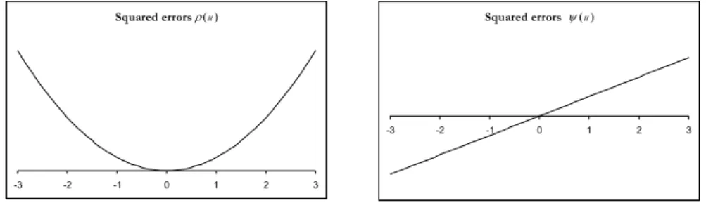
is strictly convex in θ , and the M-estimator is uniquely determined. For example, Figures 1 and 2 show ρ( )u =u2 and ( ) | |ρ u = u , respectively, together with the corresponding ( )ψ ⋅ functions. For squared errors, ρ increases at an accelerating rate, while for absolute errors it increases at a constant rate. Furthermore, for the LS function ( )ψ ⋅ is unbounded; thus LS tends to be non-robust when used with data arising from a heavy-tailed distribution. In order to obtain a robust M-estimator, only bounded influence functions have to be considered. In fact, if the M-estimator estimates the center of symmetry of p (y), then its breakdown point is 0 when ( )ψ ⋅ is an unbounded function, while it is equal to ½ when ( )ψ ⋅ is odd and bounded. Hence, the class of M-estimators contains robust as well as non-robust elements (Jurečková and Picek, 2006).Squared errors ρ(u )
-3 -2 -1 0 1 2 3
Squared errors ψ(u )
-3 -2 -1 0 1 2 3
Figure 1 – Squared function (left panel) and the corresponding derivative (right panel).
Absolute errors ρ(u )
-3 -2 -1 0 1 2 3
Absolute errors ψ(u )
-3 -2 -1 0 1 2 3
Figure 2 – Absolute function (left panel) and the corresponding derivative (right panel).
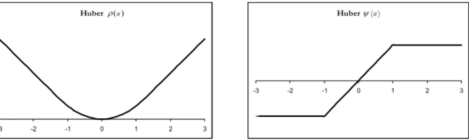
A widely used class of ρ (⋅) functions is the family of Huber’s functions. It is defined as follows: 2 2 | | , ( ) 2 | | | | , HU u if u k u k u k if u k ρ = ⎨⎧⎪ ≤ − > ⎪⎩ (9)
where k>0 is a tuning parameter allowing to distinguish small from large absolute values of u, that are transformed through a quadratic function and a linear one, respectively. This class contains ρ( )u =u2and ( ) | |ρ u =u as elements. They cor-respond to the limit cases k → ∞ and k → , respectively. 0
Figure 3 shows Huber’s function ρHU (⋅) and the corresponding function ( )ψ ⋅
for k=1. In general, small values of k produce high resistance to outliers, but at the expense of low efficiency when the errors are i.i.d. normal variables with zero mean and variance σ2. Thus, the constant k is generally selected to give reasona-bly high efficiency in the normal case. In particular, setting k = 1,345σ produces 95% asymptotic efficiency when the errors are normal, while still offering protec-tion against outliers.
A drawback of this family of functions is that they do not completely avoid the influence of large errors, as can be seen from the behavior of the influence func-tion (Figure 3, right panel).
Huber ρ(u )
-3 -2 -1 0 1 2 3
Huber ψ(u )
-3 -2 -1 0 1 2 3
Figure 3 – Huber’s function for k=1 (left panel) and the corresponding derivative (right panel). This drawback is overcome by a special class of M-estimators: the so called re-descending M-estimators. They have ( )ψ ⋅ functions that are non-decreasing near the origin, but decreasing toward 0 far from the origin. A very popular choice of
ρ (⋅) that leads to redescending M-estimators is Tukey’s bisquare family of func-tions: 2 3 1 [1 ( / ) ] | | , ( ) 1 | | , TU u k if u k u if u k ρ = ⎨⎧ − −⎪ ≤ > ⎪⎩ (10)
where k > 0 is again a tuning parameter (see Figure 4 for the special case k = 1). In order to produce a 95% asymptotic efficiency when the errors are normal, k has to be set equal to 4,685σ.
Tukey ρ(u )
-3 -2 -1 0 1 2 3
Tukey ψ(u )
-3 -2 -1 0 1 2 3
Figure 4 – Tukey’s function for k=1 (left panel) and the corresponding derivative (right panel). The redescending M-estimators are slightly more efficient than Huber’s estima-tors for several symmetric, heavy tailed distributions, but much more efficient for the Cauchy distribution. This happens because they completely reject gross out-liers, while Huber’s estimator effectively treats them as moderate outliers. There-fore, they offer an increase in robustness toward large outliers (Maronna et al., 2006). Other choices for ρ (⋅) and ( )ψ ⋅ functions have been proposed in the lit-erature on robust estimation, such as the Cauchy function, the Andrews sinus function, and a continuous, piecewise function proposed by Hampel (1974) (Jurečková and Picek, 2006).
As M-estimators are not scale equivariant, the M-estimates may depend heavily on the measurement units. In order to obtain scale equivariant M-estimates of a location parameter, several approaches have been proposed. A first intuitive solu-tion consists of modifying the minimizasolu-tion problem defined in equasolu-tion (7) as follows: 1 ˆ arg min n i i y θ θ ρ σ Θ ∈ = − ⎛ ⎞ ⎜ ⎟ ⎝ ⎠
∑
, (11)where σˆ is a previously computed dispersion estimate of the yi’s. A robust way to
obtain such an estimate may be to compute the median of the absolute values of the differences from the median (also referred to as the mean absolute deviation), divided by 0.675. This is an approximately unbiased estimator of σ if n is large and the error distribution is normal. In this situation, the breakdown point of an M-estimator of the location parameter θ obtained using a bounded and odd ( )ψ ⋅ function is still equal to ½, while the situation is more complex for redescending M-estimators with a bounded ρ (⋅) function (Maronna et al., 2006). However, Huber (1984) demonstrated that for Tukey’s bisquare function with σ estimated by the mean absolute deviation, the breakdown point of the M-estimator is ½ for all practical purposes. A second approach, based on a location-dispersion model, assumes that the probability density function p (y) is parameterized also by a dis-persion parameter. Thus, a simultaneous M-estimator of both parameters of this model may be obtained (for more details on this second approach, see Maronna et al., 2006). In general, the first approach is more robust than the second one. However, a simultaneous estimation will be useful in more general situations (e.g., in some types of multivariate analysis).
In order to stress why M-estimators are robust, it is useful to note that an M-estimate of a location parameter can be expressed as a weighted mean of the yi’s. In fact, if we define the following weight function:
( ) ( ) i i i u w u u ψ = , (12)
equation (8) can be written as
1 1 ( ) ( )( ) 0 n n i i i i i i w u u w y θ y θ = = = − − =
∑
∑
, (13)and it leads to:
1 1 ( ) ( ) n i i i n i i w u y w u θ = = =
∑
∑
. (14)This is exactly the solution that we obtain if we solve an iterated re-weighted least square problem, where weights are recomputed after each iteration. In the LS estimate, all data points are weighted equally, while the M-estimators, correspond-ing to different choices of ρ (⋅), provide adaptive weighting functions that assign smaller weights to outlying observations (Maronna et al., 2006).
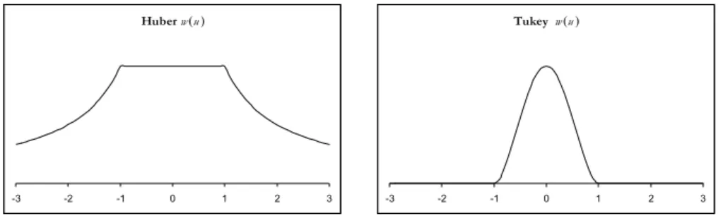
While the weighting function corresponding to Huber’s estimator declines when |u|>k, the weights for Tukey’s bisquare one decline as soon as u departs from 0 and are set equal to 0 for |u| greater than k (see Figure 5).
Huber w (u )
-3 -2 -1 0 1 2 3
Tukey w (u )
-3 -2 -1 0 1 2 3
Figure 5 – Huber’s and Tukey’s weight functions for k=1.
M-estimation methodology may be used to robustify the tree-based regression procedures proposed by Breiman et al. (1984). This result can simply be obtained by building trees whose nodes are iteratively split so as to maximize the decrease in the following objective function:
1 ( ) t T i t t i L y ρ θ = ∈ −
∑ ∑
, (15)where ρ (⋅) denotes a function chosen from the classes of functions usually used in M-estimation methodology, and θt is the corresponding M-estimate of the
loca-tion parameter in node Lt. Equation (4) and (5) are special cases of equation (15).
Thus, using the criterion defined by equation (15) in regression tree building represents a generalization of the LS and LAD regression tree-based procedures. 4. EXPERIMENTAL RESULTS
In order to evaluate the performance of the recursive procedures for con-structing the robust regression trees described in the previous section, a Monte Carlo study has been performed. Given the properties of the classes of Huber's and Tukey's functions, the study has focused particularly on the robust regression trees obtained using these two types of functions.
The recursive procedures whose split criteria are based on Huber's and Tukey's functions have been implemented in R code by suitably modifying the rpart package. For comparison purposes, also the regression trees obtained from the LS
and the LAD criteria have been included in the study. The main results obtained from two simulation experiments, in which the datasets have been generated ac-cording to two different models, are described and discussed in this section. As already stressed, the use of Huber's and Tukey's criteria requires the choice of a value for the constant k. In both simulation experiments, k has been set equal to 1,345σ for Huber's function and equal to 4,685σ for Tukey's one, where the scale parameter σ has been estimated by σˆ=MAD/0.6745, where MAD is the median of the absolute deviations of the LAD tree residuals from their median.
Simulation experiment 1
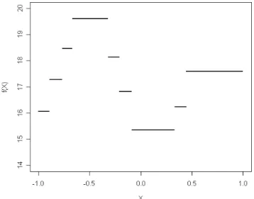
The model used to generate the datasets in the first simulation study is Y = f (X1) + u , where f (⋅) is the step function with 9 steps illustrated in Figure 6, and X1 is a random variable uniformly distributed in D = [-1; 1]. The error term u has a probability density function p (u) given by a mixture of two normal density functions; a small proportion of the observations, equal to δ, is generated by the normal model with zero mean and a standard deviation equal to 10, while the re-maining proportion (1 - δ ) is generated by the normal model with zero mean and a standard deviation τ 10. That is: u ~ (1−δ) (0, )N τ +δN(0,10). Thus, p (u) de-pends on the parameters δ and τ. The former represents the proportion of con-taminated observations. If δ = 0 all the observations will be generated by the same distribution and the simulated datasets will not contain outliers. When δ > 0, p (u) will have heavy tails and outlying observations will be present in the data. The latter parameter τ represents the standard deviation of the bulk of the data.
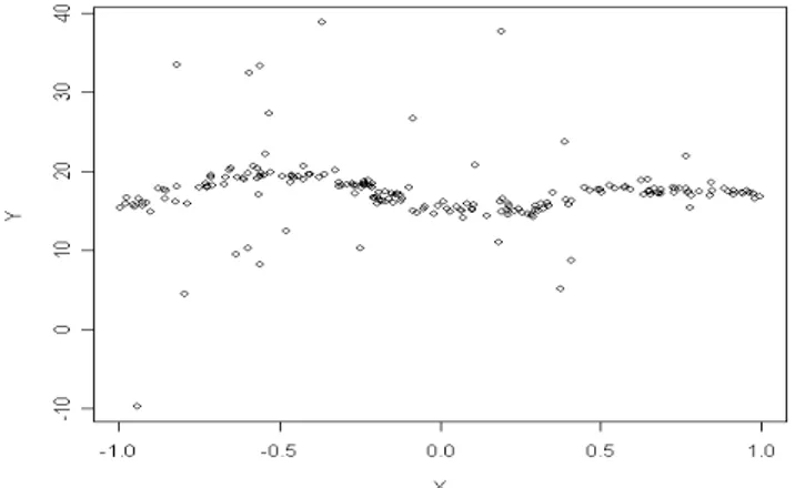
Figure 7 shows a sample of n = 200 units generated from the described model for δ = 0.15 and τ = 0.5; as can be seen, some outlying observations are present
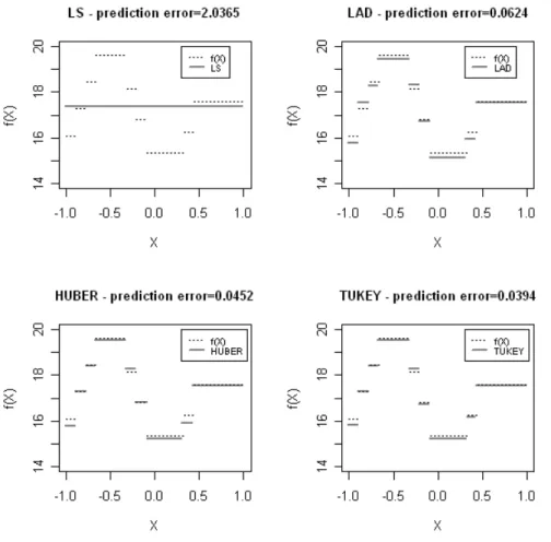
in the dataset. Figure 8 illustrates the regression trees obtained by applying the recursive procedures based on the LS, LAD, Huber's and Tukey's split criteria to the learning sample illustrated in Figure 7. The LS regression tree has only one terminal node, thus producing a very bad approximation of the true step func-tion. The prediction error of this tree is equal to 2.0365. This value is obtained as the mean of the squared differences between the values of the true step function f (⋅) used to generate the data and the values of the approximating function ˆ( )f ⋅ given by the tree, evaluated on a sequence of 10000 values of the predictor. The regression trees obtained from the other three split criteria all have nine terminal nodes, but with slightly different partitions of the predictor space D and slightly different values of the θt. From the comparison of the prediction errors of these
trees, the best approximation of the true function is given by the tree obtained using Tukey's split criterion.
Figure 7 – Sample of 200 units generated from the model used in the first simulation experiment, with δ = 0.15 and τ = 0.5.
In the simulation experiment, the effects of the following three factors were evaluated: the proportion of contaminated observations (δ, with levels 0, 0.05, 0.10, 0.15); the standard deviation of the bulk of the data (τ , with levels 0.5 and 1); and the sample size (n, with levels 200 and 400). For each combination of these factors, 50 learning samples and 50 test samples consisting of n units each were generated from the described model. Then, each couple of learning and test set was used to construct and prune regression trees through the four considered strategies. Furthermore, each regression tree was evaluated with a special empha-sis on the following two aspects: the number of terminal nodes (tree size) and the prediction error.
Tables 1 and 2 show the means (and the standard deviations in brackets) of the tree sizes and the prediction errors over the 50 replications, for random (training and test) samples of 200 and 400 units, respectively. As expected, when no out-liers are present in the data (δ = 0), the lowest mean prediction errors are
ob-tained with the LS regression trees. In such a situation, the LAD criterion seems to perform slightly worse than Huber's and Tukey's. As far as the tree size is con-cerned, the four strategies are equivalent. In the presence of contaminated obser-vations, the mean prediction errors of the LS trees dramatically increase, especially when τ = 0.5. Furthermore, using the LS criterion leads to a reduction in the tree sizes, which may be related to the increase in the prediction errors. Among the three robust criteria, Tukey's trees achieve the best performance: they show the lowest mean prediction errors in all the situations in which contaminated obser-vations are present in the data. Moreover, their performances are slightly affected by the value of δ . Huber's trees reach similar results only when δ = 0.05, while when δ = 0.1 and δ = 0.15, the differences between Huber's and Tukey's strate-gies increase. As far as LAD trees are concerned, they have mean prediction errors lower than LS trees but higher than the other two robust alternatives.
Figure 8 – Regression trees obtained from the analysis of the sample illustrated in Figure 7 through four different split criteria.
TABLE 1
Mean and standard deviation (in brackets) of the tree sizes and the prediction errors over 50 replications n=200
τ = 0.5 τ = 1
Tree size Prediction error Tree size Prediction error
LS 9.30 (1.06) 0.087 (0.035) 8.92 (2.22) 0.220 (0.053) δ = 0 LAD 9.14 (1.23) 0.104 (0.040) 9.18 (3.34) 0.262 (0.067) HUBER 9.46 (1.55) 0.094 (0.041) 8.60 (2.39) 0.239 (0.070) TUKEY 9.26 (1.66) 0.102 (0.040) 8.34 (2.71) 0.245 (0.078) LS 6.22 (2.71) 0.617 (0.361) 6.30 (3.32) 0.701 (0.354) δ = 0.05 LAD 9.48 (1.75) 0.124 (0.042) 8.26 (2.71) 0.297 (0.072) HUBER 9.08 (1.35) 0.113 (0.038) 7.84 (2.47) 0.256 (0.063) TUKEY 9.24 (1.87) 0.105 (0.042) 7.98 (2.01) 0.241 (0.058) LS 4.80 (1.99) 1.036 (0.391) 4.88 (2.32) 1.102 (0.385) δ = 0.10 LAD 9.32 (1.92) 0.125 (0.049) 8.30 (2.68) 0.293 (0.099) HUBER 9.46 (1. 90) 0.126 (0.054) 8.02 (2.38) 0.287 (0.088) TUKEY 9.44 (1.73) 0.096 (0.042) 8.76 (2.74) 0.243 (0.065) LS 3.84 (2.15) 1.414 (0.530) 3.82 (2.05) 1.102 (0.510) δ = 0.15 LAD 9.00 (1.62) 0.152 (0.058) 7.86 (2.68) 0.293 (0.084) HUBER 9.12 (1.62) 0.160 (0.061) 7.12 (1.90) 0.286 (0.094) TUKEY 9.08 (1.60) 0.116 (0.042) 8.28 (2.84) 0.243 (0.079) TABLE 2
Mean and standard deviation (in brackets) of the tree sizes and the prediction errors over 50 replications n=400
τ = 0.5 τ = 1
Tree size Prediction error Tree size Prediction error
LS 9.28 (0.64) 0.033 (0.016) 9.40 (2.31) 0.110 (0.038) δ = 0 LAD 9.86 (2.13) 0.041 (0.016) 9.48 (2.17) 0.133 (0.054) HUBER 9.24 (0.56) 0.035 (0.016) 9.88 (2.16) 0.112 (0.043) TUKEY 9.80 (1.25) 0.038 (0.017) 9.72 (1.93) 0.114 (0.045) LS 5.38 (2.00) 0.427 (0.161) 6.04 (3.35) 0.494 (0.172) δ = 0.05 LAD 9.64 (1.14) 0.047 (0.020) 9.44 (2.37) 0.153 (0.045) HUBER 9.44 (1.22) 0.043 (0.020) 9.48 (2.48) 0.138 (0.049) TUKEY 9.56 (0.86) 0.038 (0.014) 9.10 (1.40) 0.123 (0.037) LS 5.60 (3.99) 0.687 (0.364) 4.64 (1.58) 0.648 (0.327) δ = 0.10 LAD 9.72 (1.18) 0.056 (0.017) 9.80 (3.68) 0.171 (0.056) HUBER 9.52 (1.07) 0.053 (0.019) 8.74 (1.41) 0.148 (0.053) TUKEY 9.26 (0.60) 0.043 (0.014) 9.78 (3.44) 0.125 (0.045) LS 4.72 (2.65) 0.859 (0.358) 4.60 (1.78) 0.930 (0.359) δ = 0.15 LAD 9.62 (1.19) 0.070 (0.048) 9.52 (3.25) 0.194 (0.073) HUBER 9.40 (0.83) 0.070 (0.044) 8.88 (2.44) 0.197 (0.077) TUKEY 9.70 (1.74) 0.049 (0.018) 9.24 (2.21) 0.145 (0.044) Simulation experiment 2
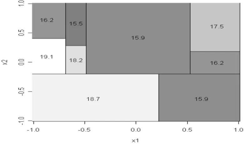
In the second simulation experiment, the datasets were generated according to the model Y = f (X1, X2)+u, where f (⋅) is a step function with 9 steps and X1 and X2 are i.i.d. random variables uniformly distributed in [-1; 1]. Figure 9 shows the partition of the predictor space D = [-1; 1] [-1; 1]× and the value of Y for each element of the partition. The probability density function of the error term u is the same as the one used in the previous experiment, that is
(1−δ) (0, )N τ +δN(0,10).
The effects of the same factors considered in the previous experiments were evaluated also in this second one, e.g. the proportion δ of contaminated
observa-tions; the standard deviation of the bulk of the data τ; and the sample size n. The levels of the first two factors are the same ones previously examined, while the sample size n was set equal to 1000 and 1500 in order to take into account the in-creased dimensionality of the predictor space.
For each combination of these factors, 50 learning samples and 50 test samples of n units were generated from the described model, and used to construct pruned regression trees through the four considered strategies. As in the previous experiment, the means and the standard deviations of the tree sizes and the pre-diction errors over the 50 replications for the four considered strategies were computed for random samples of 1000 and 1500 units (see Tables 3 and 4).
Figure 9 – Partition of D and values of Y for the model used in the simulation experiment 2.
TABLE 3
Mean and standard deviation (in brackets) of the tree sizes and the prediction errors over 50 replications n=1000
τ= 0.5 τ= 1
Tree size Prediction error Tree size Prediction error
LS 11.78 (2.32) 0.062 (0.035) 10.38 (1.97) 0.105 (0.042) δ = 0 LAD 12.76 (2.88) 0.092 (0.039) 10.18 (2.47) 0.144 (0.051) HUBER 12.74 (2.74) 0.080 (0.032) 10.32 (2.29) 0.118 (0.038) TUKEY 11.94 (2.49) 0.091 (0.047) 10.26 (2.14) 0.122 (0.040) LS 8.16 (3.29) 0.348 (0.144) 7.78 (2.62) 0.372 (0.149) δ = 0.05 LAD 12.64 (2.64) 0.105 (0.039) 9.98 (2.43) 0.159 (0.042) HUBER 12.74 (2.38) 0.089 (0.034) 9.84 (2.43) 0.130 (0.047) TUKEY 12.40 (2.52) 0.089 (0.045) 9.98 (2.45) 0.124 (0.036) LS 6.22 (2.15) 0.553 (0.199) 6.22 (2.45) 0.596 (0.192) δ = 0.10 LAD 12.72 (3.59) 0.108 (0.039) 9.58 (2.61) 0.155 (0.056) HUBER 11.32 (2.62) 0.104 (0.041) 9.78 (2.45) 0.142 (0.052) TUKEY 12.20 (2.30) 0.093 (0.052) 10.24 (2.38) 0.127 (0.046) LS 5.40 (1.88) 0.723 (0.243) 5.00 (2.01) 0.725 (0.237) δ = 0.15 LAD 11.34 (2.38) 0.112 (0.045) 9.68 (2.61) 0.168 (0.058) HUBER 10.72 (2.06) 0.102 (0.048) 9.04 (2.01) 0.161 (0.048) TUKEY 12.50 (2.47) 0.106 (0.057) 9.84 (1.74) 0.136 (0.047)
TABLE 4
Mean and standard deviation (in brackets) of the tree sizes and the prediction errors over 50 replications n=1500
τ= 0.5 τ= 1
Tree size Prediction error Tree size Prediction error
LS 10.88 (1.71) 0.033 (0.022) 10.28 (1.68) 0.059 (0.026) δ = 0 LAD 12.86 (2.43) 0.049 (0.023) 10.90 (2.42) 0.084 (0.035) HUBER 12.70 (2.07) 0.045 (0.024) 10.56 (2.08) 0.066 (0.028) TUKEY 12.72 (2.19) 0.047 (0.025) 10.80 (2.24) 0.072 (0.035) LS 8.26 (2.54) 0.252 (0.126) 7.70 (1.92) 0.279 (0.134) δ = 0.05 LAD 12.56 (2.18) 0.054 (0.030) 10.34 (2.50) 0.093 (0.036) HUBER 12.02 (1.58) 0.049 (0.024) 10.38 (1.77) 0.083 (0.034) TUKEY 13.12 (2.46) 0.052 (0.024) 10.34 (1.75) 0.082 (0.038) LS 6.96 (1.97) 0.399 (0.175) 6.88 (1.96) 0.421 (0.190) δ = 0.10 LAD 12.24 (2.13) 0.064 (0.034) 10.42 (2.47) 0.103 (0.045) HUBER 11.80 (1.92) 0.058 (0.030) 9.92 (2.04) 0.091 (0.037) TUKEY 12.52 (1.98) 0.060 (0.036) 10.24 (2.26) 0.083 (0.044) LS 6.26 (2.16) 0.570 (0.221) 6.08 (1.85) 0.581 (0.208) δ = 0.15 LAD 12.00 (1.86) 0.076 (0.034) 10.10 (2.52) 0.123 (0.051) HUBER 11.14 (1.73) 0.072 (0.033) 9.92 (2.16) 0.113 (0.048) TUKEY 12.50 (2.07) 0.064 (0.028) 10.42 (1.80) 0.083 (0.031)
As in the previous experiment, when δ = 0, the LS and the LAD regression trees have the lowest and the highest mean prediction errors, respectively. As far as the tree size is concerned, the four strategies overestimate in a very similar way the number of steps for the unknown function f (⋅). In the presence of contaminated observations, the performance of the LS trees dramatically worsen, especially when τ = 0.5. As the means of the tree sizes in Tables 3 and 4 show, they under-estimate the number of steps of f (⋅), for each combination of n, τ, δ ≠ . When 0 contaminated observations are present in the data, all the three robust criteria lead to trees able to accurately predict f (⋅), but LAD trees never achieve the best performance. Huber's and Tukey's trees show similar performances, but Tukey’s ones seem to outperform the others more often.
5. CONCLUSIONS
In this paper a new recursive partitioning procedure for building robust regres-sion trees is described, based on M-estimation methodology. It relies on robust split criteria that allow to downweight outliers when calculating the measure of within-node impurity.
The results obtained on simulated datasets showed the usefulness and the effi-cacy of this approach with respect to the presence of outlying values in the de-pendent variable. In particular, when data is outlier free, the proposed robust re-gression trees performed more similarly to LS trees than LAD trees. Furthermore, with a small proportion of contaminated observations, they yielded better results than LAD and LS trees. Moreover, trees based on Tukey’s function performed slightly better than the ones based on Huber’s function.
Several issues related to the current work deserve further research. Firstly, other data-generating schemes need to be considered, characterized by different
distributions of the error term (for example, heavy-tails or asymmetric distribu-tions). Secondly, issues concerning the choice of the tuning parameter k should be examined in more depth. Moreover, different robust estimation procedures, such as L-estimation and R-estimation methodologies, could be evaluated in or-der to or-derive other split criteria and other estimators of function f (⋅) in each ele-ment of the final partition of the predictor space. Finally, only the effect of outly-ing values in the dependent variable was addressed. As recursive partitionoutly-ing pro-cedures rely only on the ranks of predictor values, it is expected that they should be less prone to distortions from outliers in the predictor values. The analysis of real and simulated data sets with these characteristics may be useful to have a deeper insight into this issue.
Department of Statistics GIULIANO GALIMBERTI
University of Bologna MARILENA PILLATI
GABRIELE SOFFRITTI
REFERENCES
J.N. ADICHIE (1967), Estimates of regression parameters based on rank tests, “The Annals of
Mathematical Statistics”, 38, pp. 894-904.
A. ATKINSON, M. RIANI (2000), Robust Diagnostic Regression Analysis. Springer, New York. L. BRIEMAN, J. FRIEDMAN, R. OLSHEN, C. STONE (1984), Classification and regression trees. Wadsworth,
Belmont.
R. CHAMBERS, A. HENTGES, X. ZHAO (2004), Robust automatic methods for outlier and error detec-tion, “Journal of the Royal Statistical Society”, A, 167, pp. 323-339.
M. COSTA, G. GALIMBERTI, A. MONTANARI(2006),Binary segmentation methods based on Gini index: a
new approach to the multidensional analysis of income inequalities,“Statistica & Applicazioni”, IV, pp. 19-37.
R.V. HOGG, R.H. RANDLES(1975), Adaptive distribution-free regression methods and their applications,
“Technometrics”, 17, pp. 399-407.
F.R. HAMPEL(1974), The influence curve and its role in robust estimation, “Journal of the American
Statistical Association”, 69, pp. 383-393.
P.J. HUBER(1964), Robust estimation of a local parameter, “The Annals of Mathematical
Statis-tics”, 35, pp. 73-101.
P.J. HUBER(1981), Robust Statistics, Wiley, New York.
P.J. HUBER(1984), Finite sample breakdown of M- and P-estimators, “Annals of Statistics”, 12,
pp. 119-126.
L.A. JAECKEL(1972), Estimating regression coefficients by minimizing the dispersion of the residuals,
“The Annals of Mathematical Statistics”, 43, pp. 1449-1458.
J. JUREČKOVÁ(1977), Asymptotic relations of M-estimates and R-estimates in linear regression models,
“Annals of Statistics”, 5, pp. 464-472.
J. JUREČKOVÁ, J. PICEK(2006),Robust Statistical Methods with R. Chapman & Hall/CRC, Boca
Raton.
R. KOENKER, G.J. BASSETT(1978), Regression quantiles, “Econometrica”, 46, pp. 33-50.
R. KOENKER, P. HAMMOND, A. HOLLY(EDS.)(2005),Quantile Regression, Cambridge University Press, Cambridge.
R.A. MARONNA, R.D. MARTIN, V.J. YOHAI(2006), Robust Statistics. Theory and Methods, Wiley, New
D.C. MONTGOMERY, E.A. PECK, G.G. VINING (2006), Introduction to Linear Regression Analysis,
Fourth edition. Wiley, New York.
P.J. ROUSSEEUW(1984), Least median of squares regression, “Journal of the American Statistical
Association”, 79, pp. 871-880.
P.J. ROUSSEEUW, A.M. LEROY(1987), Robust Regression and Outlier Detection. Wiley, New York.
SUMMARY
Robust regression trees based on M-estimators
The paper addresses the problem of robustness of regression trees with respect to out-lying values in the dependent variable. New robust tree-based procedures are described, which are obtained by introducing in the tree building phase some objective functions already used in the linear robust regression approach, namely Huber’s and Tukey’s bis-quare functions. The performance of the new procedures is evaluated through a Monte Carlo experiment.