A gravity model of migration between ENC and EU

A GRAVITY MODEL OF MIGRATION BETWEEN

ENC AND EU

RAUL RAMOS

_{, JORDI SURIÑACH}

AQR-IREA, University of Barcelona; Facultat d'Economia i Empresa,

Universitat de Barcelona, Barcelona, Spain

ABSTRACT

Due to its ageing population and low birth rates, the European Union (EU) will need to import foreign labour in the next decades. In this context, the EU neighbouring countries (ENC) are the main countries of origin and transit of legal and irregular migration towards Europe. Their economic, cultural, and historical links also make them an important potential source of labour. The objective of this paper is to analyse past and future trends in ENC-EU bilateral migration relationships. With this aim, we specify and estimate a gravity model for nearly 200 countries between 1960 and 2010. Next, we use the model to obtain medium-run migration forecasts. Our results show a clear increase in migratory pressures from ENC to the EU in the near future, but probably lower than initially expected.

Keywords: Bilateral migration, EU neighbouring countries, gravity model, push and pull migration factors

INTRODUCTION AND OBJECTIVES

The free movement of workers is one of the fundamental principles upon which the European Union (EU) was founded, and it is also presents as a future goal in bilateral negotiations with most neighbouring countries. As recognised in the Europe 2020 strategy, the EU has a clear demographic challenge for the next decades. The EU will need to import foreign labour in response to gloomy demographic forecasts, in the context of ageing populations, low birth-rates, and prospects of a collapsing social security system, but it is also necessary to remain competitive in a global context. This means that the EU has to attract and retain the more skilled migrants.

Attracting and retaining skilled migrants requires improving the current control over migration flows, and this is one of the reasons why the European migration policy was integrated into the European Neighbourhood Policy (ENP) from the very beginning. The EU neighbouring countries are the main countries of origin and transit of legal and illegal migration towards Europe. Moreover, their geographical proximity, economic, cultural, and historical links make them an important potential source of labour. In fact, nearly all Action Plans, the main tool of the ENP, include proposals for action in areas such as border management and management of migration flows. The EU proposed actions in the field of migration, asylum, visa policies, trafficking and smuggling, illegal migration, and police cooperation.

The objective of this paper is to analyse past and future trends in ENC-EU bilateral economic migration. With this aim, two empirical analyses are carried out. First, we specify and estimate a gravity model for nearly 200 countries between 1960 and 2010, and next, we use the model to obtain medium-run migration forecasts.

The rest of the paper is structured as follows: in the next section, the main population and migration trends from and to ENC and Russia are described; then, the dataset and the gravity models used in the analysis are presented; and finally, we conclude with some final remarks.

POPULATION AND MIGRATION TRENDS FROM AND TO ENC

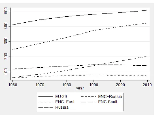
In this section, we provide a brief description of population and migration trends from and to the ENC plus Russia. We use statistical data from the World Bank Development Indicators. As can be seen in figure 1, the population of the ENC plus Russia is currently more than 400 million people, while in the 1960s the population in the ENC-South (Algeria, Egypt, Israel, Jordan, Lebanon, Libya, Morocco, Syria, and Tunisia) was around 60 million people—a similar figure to the population of ENC-East (Armenia, Azerbaijan, Belarus, Georgia, Moldova and Ukraine). Currently, population of ENC-South is substantially higher than in ENC-East: 204 million people vs. 75 million. The Russian population has also experienced very important growth, from 250 million people in 1960 to 420 million people in 2010. Population growth has been clearly higher in Russia and the ENC-South than in the EU-29, where population increased from 400 million people in 1960 to 500 million people in 2010.

Figure 1. Population trends in the EU, ENC and Russia

Note: Palestinian territory is not considered due to the lack of data. Data expressed in millions of inhabitants.

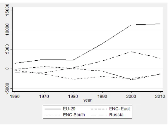
As shown in figure 2, and according to data from the World Bank Development Indicators, there has been a very high heterogeneity regarding migration trends in ENC countries in the last 50 years. The EU-29 and Russia have been net receivers from 1980 onwards, although the trend seems to be stabilising according to the latest data. However, the situation has been clearly different from ENC countries. The ENC-South has acted as a net sender throughout the period, and migration from the ENC-East was nearly inexistent until the 1990s, after which emigration became a constant feature, according to World Bank data.

Figure 2. Accumulated net migration by decades in the EU, ENC and Russia

Note: Palestinian territory is not considered due to the lack of data. Data expressed in thousands of individuals.

Source: Own elaboration from World Bank Development Indicators.

A similar heterogeneity is observed at the country level as shown in tables 2 and 3. While some countries, such as Israel during the whole period or Russia over the last 30 years, have been net receivers, other countries, such as Belarus, Egypt, or Tunisia, have clearly lost population due to migration during the considered period. An additional interesting feature of migration from the ENC is that it is highly concentrated in some destination countries due to geographical proximity or strong political, economic, or colonialist linkages (see table 4). For instance, most migrants from Algeria or Tunisia go to France and most migrants from ENC-East go to Russia. In fact, one interesting result is that European Union countries are not always the main destination of migrants

from ENC: for instance, emigrants from Egypt choose Saudi Arabia as their first destination, those from Lebanon prefer to migrate to the United States, or those from Syria go to Jordan, Kuwait, or Saudi Arabia. Migratory movements among ENC members have been quite relevant in the more recent period. Currently, about 10% of the total population in ENC-East was born abroad, while this figure is around 5% in ENC-South and Russia. In the EU-29, the stock of the foreign-born population is around 10%.

DATA SOURCES

It is a difficult task to collect data on homogeneous international migration for a large number of countries (Fertig and Schmidt, 2000; Crespo-Cuaresma et al., 2013). There are problems of data availability and difficulties in collecting comparable statistical information across countries. From a comparative analysis of currently available datasets, the most complete source on bilateral migration seems to be World Bank Bilateral Migration Database 1960-2000 completed with the World Bank Bilateral Migration Matrix 2010 (Özden et al, 2011). It includes data for more than 200 countries for a long time period starting in 1960 and ending in 2010, and it provides information on bilateral migration stocks for every 10 years: 1960, 1970, 1980, 1990, 2000, and 2010. Over 1,000 census and population register records are combined to construct decennial matrices corresponding to the last five completed census rounds. Immigrants are identified using the foreign-born criteria, but as the focus is on economic migrants, refugees are not considered in the analysis with the only exception of Palestine (Özden et al., 2011, page 27, footnote 21). The only problem with this dataset is that it provides information on stocks rather than on flows. However, migration stocks data have been used in several studies such as Ortega and Peri (2009), Brücker and Siliverstovs (2006), and Grogger and Hanson (2011) among others. Moreover, as highlighted by Brücker and Siliverstovs (2006), the analysis of stocks can be interpreted as a representation of a long-term equilibrium, and as data on immigration stocks are based on national censuses, they are probably of higher quality than those that report annual immigrant flows. Censuses deal with unambiguous net permanent moves and reduce the undercounting of undocumented immigrants. However, the dataset only allows consideration of aggregate stocks with no possibility of taking into account gender, age, schooling levels, or years of residence in the host country.

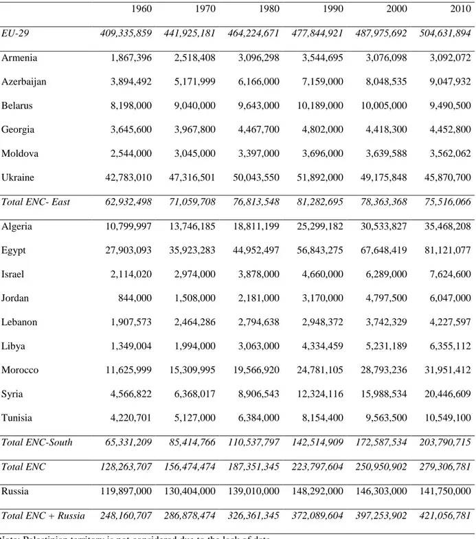
Table 1. Population trends. Country analysis. 1960 1970 1980 1990 2000 2010 EU-29 409,335,859 441,925,181 464,224,671 477,844,921 487,975,692 504,631,894 Armenia 1,867,396 2,518,408 3,096,298 3,544,695 3,076,098 3,092,072 Azerbaijan 3,894,492 5,171,999 6,166,000 7,159,000 8,048,535 9,047,932 Belarus 8,198,000 9,040,000 9,643,000 10,189,000 10,005,000 9,490,500 Georgia 3,645,600 3,967,800 4,467,700 4,802,000 4,418,300 4,452,800 Moldova 2,544,000 3,045,000 3,397,000 3,696,000 3,639,588 3,562,062 Ukraine 42,783,010 47,316,501 50,043,550 51,892,000 49,175,848 45,870,700

Total ENC- East 62,932,498 71,059,708 76,813,548 81,282,695 78,363,368 75,516,066

Algeria 10,799,997 13,746,185 18,811,199 25,299,182 30,533,827 35,468,208 Egypt 27,903,093 35,923,283 44,952,497 56,843,275 67,648,419 81,121,077 Israel 2,114,020 2,974,000 3,878,000 4,660,000 6,289,000 7,624,600 Jordan 844,000 1,508,000 2,181,000 3,170,000 4,797,500 6,047,000 Lebanon 1,907,573 2,464,286 2,794,638 2,948,372 3,742,329 4,227,597 Libya 1,349,004 1,994,000 3,063,000 4,334,459 5,231,189 6,355,112 Morocco 11,625,999 15,309,995 19,566,920 24,781,105 28,793,236 31,951,412 Syria 4,566,822 6,368,017 8,906,543 12,324,116 15,988,534 20,446,609 Tunisia 4,220,701 5,127,000 6,384,000 8,154,400 9,563,500 10,549,100 Total ENC-South 65,331,209 85,414,766 110,537,797 142,514,909 172,587,534 203,790,715 Total ENC 128,263,707 156,474,474 187,351,345 223,797,604 250,950,902 279,306,781 Russia 119,897,000 130,404,000 139,010,000 148,292,000 146,303,000 141,750,000

Total ENC + Russia 248,160,707 286,878,474 326,361,345 372,089,604 397,253,902 421,056,781

Note: Palestinian territory is not considered due to the lack of data Source: Own elaboration from World Bank Development Indicators.

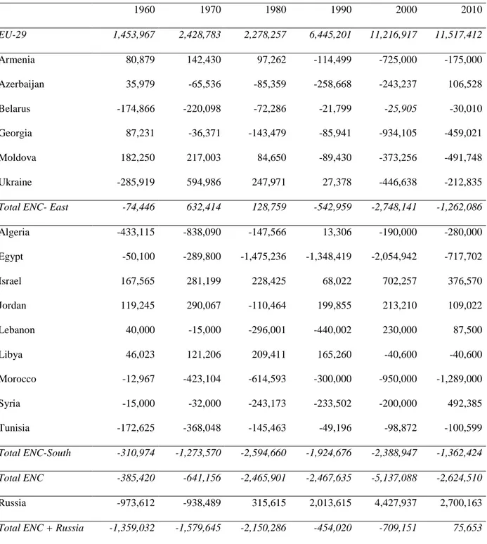
Table 2. Accumulated net migration by decades. Country analysis 1960 1970 1980 1990 2000 2010 EU-29 1,453,967 2,428,783 2,278,257 6,445,201 11,216,917 11,517,412 Armenia 80,879 142,430 97,262 -114,499 -725,000 -175,000 Azerbaijan 35,979 -65,536 -85,359 -258,668 -243,237 106,528 Belarus -174,866 -220,098 -72,286 -21,799 -25,905 -30,010 Georgia 87,231 -36,371 -143,479 -85,941 -934,105 -459,021 Moldova 182,250 217,003 84,650 -89,430 -373,256 -491,748 Ukraine -285,919 594,986 247,971 27,378 -446,638 -212,835

Total ENC- East -74,446 632,414 128,759 -542,959 -2,748,141 -1,262,086

Algeria -433,115 -838,090 -147,566 13,306 -190,000 -280,000 Egypt -50,100 -289,800 -1,475,236 -1,348,419 -2,054,942 -717,702 Israel 167,565 281,199 228,425 68,022 702,257 376,570 Jordan 119,245 290,067 -110,464 199,855 213,210 109,022 Lebanon 40,000 -15,000 -296,001 -440,002 230,000 87,500 Libya 46,023 121,206 209,411 165,260 -40,600 -40,600 Morocco -12,967 -423,104 -614,593 -300,000 -950,000 -1,289,000 Syria -15,000 -32,000 -243,173 -233,502 -200,000 492,385 Tunisia -172,625 -368,048 -145,463 -49,196 -98,872 -100,599 Total ENC-South -310,974 -1,273,570 -2,594,660 -1,924,676 -2,388,947 -1,362,424 Total ENC -385,420 -641,156 -2,465,901 -2,467,635 -5,137,088 -2,624,510 Russia -973,612 -938,489 315,615 2,013,615 4,427,937 2,700,163

Total ENC + Russia -1,359,032 -1,579,645 -2,150,286 -454,020 -709,151 75,653

Note: Palestinian territory is not considered due to the lack of data Source: Own elaboration from World Bank Development Indicators.

Table 3. Immigrant stock as a percentage of population. Country analysis 1960 1970 1980 1990 2000 2010 EU-29 3,7% 4.4% 4.7% 5.7% 7.3% 9.4% Armenia 18.6% 18.7% 10.5% Azerbaijan 5.0% 4.3% 2.9% Belarus 12.3% 11.2% 11.5% Georgia 7.0% 4.9% 3.8% Moldova 15.7% 13.0% 11.5% Ukraine 13.3% 11.2% 11.5%

Total ENC- East 12.4% 10.5% 9.9%

Algeria 4.0% 1.2% 1.0% 1.1% 0.8% 0.7% Egypt 0.8% 0.6% 0.4% 0.3% 0.3% 0.3% Israel 56.1% 47.4% 36.9% 35.0% 35.9% 38.6% Jordan 45.7% 35.3% 37.2% 36.2% 40.2% 49.2% Lebanon 7.9% 7.7% 8.6% 17.8% 18.5% 17.9% Libya 3.6% 6.1% 10.1% 10.6% 10.7% 10.7% Morocco 3.4% 0.8% 0.4% 0.2% 0.2% 0.2% Syria 6.0% 5.8% 5.6% 5.6% 5.8% 10.8% Tunisia 4.0% 1.0% 0.6% 0.5% 0.4% 0.3% Total ENC-South 5.0% 3.7% 3.4% 3.5% 4.0% 5.0% Total ENC 6.7% 6.0% 6.3% Russia 7.8% 8.1% 8.7%

Total ENC + Russia 7.1% 6.8% 7.1% Note: Palestinian territory is not considered due to the lack of data

Table 4. Main destination countries of emigrants from ENC + Russia in 2010

Source country Main destination countries (Percentage of total migrant stocks in 2010 above or equal 5% - EU as a reference) Armenia Russia (56.7%), United States (8.9%), Ukraine (6.1%), Azerbaijan (4.9%) – EU (7.2%)

Azerbaijan Russia (60.5%), Armenia (11.5%), Ukraine (6.5%) – EU (2.1%) Belarus Russia (54.3%), Poland (6.4%) Ukraine (15.6%) – EU (9.1%)

Georgia Russia (60.9%), Armenia (7.2%), Ukraine (6.8%), Greece (4.0%) – EU (9.1%) Moldova Russia (36.9%), Ukraine (21.9%), Italy (11.6%), Romania (5.0%) – EU (25%) Ukraine Russia (55.9%), Poland (5.1%), United States (5.1%) – EU (15.3%)

Algeria France (75.5%), Spain (5.2%) – EU (89.0%)

Egypt Saudi Arabia (26.9%), Jordan (22.8%), Libya (10.6%), Kuwait (8.5%) – EU (5.7%) Israel West Bank and Gaza (64.3%), United States (14.6%) – EU (6.2%)

Jordan West Bank and Gaza (50.3%), Saudi Arabia (23.5%) – EU (4.5%)

Lebanon United States (19.6%), Australia (14.4%), Canada (13.2%), Germany (9.3%) Saudi Arabia (8.8%), France (6.8%) - EU (28.9%) Libya Israel (25.9%), United Kingdom (11.0%), Chad (10.1%), United States (9.8%) Jordan (7.3%), Egypt (6.6%) - EU (24.6%) Morocco France (27.9%), Spain (25.8%), Italy (15.8%), Israel (8,1%), Belgium (5.7%), Netherlands (5.5%) – EU (85.4%)

Syria Jordan (30.6%), Kuwait (13.0%), Saudi Arabia (11.8%), United States (7.1%) – EU (11.5%) Tunisia France (46.4%), Italy (18.7%), Libya (13.0%), Germany (5.7%) – EU (75.58%)

Russia Ukraine (33.4%), Kazakhstan (20.2%), Israel (6.5%), Belarus (6.2%) – EU (9.9%) Note: Palestinian territory is not considered due to the lack of data.

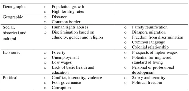
In addition to immigration stocks, a number of traditional variables related to pull and push factors of migration have been considered in order to explain bilateral migration. Table 5 summarises the different push and pull factors identified in the literature. The determinants of migration are related to demographic, geographic, social, cultural, economic, and political characteristics of both origin and destination countries. As our objective is not to explore the influence of push and pull factors on migration but to predict future movements, we only focus on a subset of these factors. In particular, and following a similar approach to Kim and Cohen (2010), we investigate the role of demographic, geographic, and historical variables and relative differences in GDP per capita. Data for these additional variables have been collected from the CEPII Geodist dyadic dataset (Head et al., 2010) and the CEPII gravity dataset (Head and Mayer, 2013). Geographical distance has been defined as the distance between the two capital cities of immigrants’ origin and destination countries using the great circle formula for cities’ latitude and longitude. Dummy variables indicating whether the two countries are contiguous, share a common language, have had a common colonizer after 1945, have ever had a colonial link, have had a colonial relationship after 1945, or are currently in a colonial relationship have been included. There are two common languages dummies, the first based on the fact that two countries share a common official language, and the other set to one if a language is spoken by at least 9% of the population in both countries.

Table 5. Migration pull and push factors

Push factors Pull factors Demographic o Population growth

o High fertility rates Geographic o Distance

o Common border Social,

historical and cultural

o Human rights abuses o Discrimination based on

ethnicity, gender and religion

o Family reunification o Diaspora migration

o Freedom from discrimination o Common language

o Colonial relationship Economic o Poverty

o Unemployment o Low wages

o Lack of basic health and education

o Prospects of higher wages o Potential for improved

standard of living o Personal or professional

development Political o Conflict, insecurity, violence

o Poor governance o Corruption

o Safety and security o Political freedom Source: Adapted from Praussello (2011)

GDP and population data from the CEPII’s gravity dataset have been updated using data from the World Bank Development Indicators and the same definitions as in the original source. Forecasts for GDP and population for 2020 have been obtained from the International Monetary Fund World Economic Outlook database (October 2015 edition).

After some adjustments related to missing country codes and equivalences between the datasets, our potential sample of bilateral migration stocks will include 199,836 origin-destination observations from 183 countries, and 6 time periods (183*183-183=33,306*6=199,836). However, due to missing values of bilateral migration stocks for 2010, our final sample includes 181,888 observations. When GDP differences between destination and origin countries are considered, the sample further reduces to 141,112 observations due to additional missing values in these variables.

EMPIRICAL ANALYSIS

There are many theoretical hypotheses and models concerning the determinants of migration. Gravity models were initially based on Newton’s gravity law, but recent contributions have also provided microfoundations in the context of migration analysis (Grogger and Hanson, 2011). These models have been widely used in the empirical analysis of migration due to their relatively good forecasting performance (Fertig and Schmid, 2000; Karemera et al., 2000 or Kim and Cohen, 2010; among others). In particular, migration stocks (or flows) between two countries are supposed to increase with their size and decay with the distance between the two countries. Usually, the most representative variable of the size of countries is population. Therefore, it is expected that migration is a positive function of population size of the host and home country and a negative function of distance (which controls for migration costs). As Santos-Silva and Tenreyro (2006) and Martinez-Zarzoso (2013) highlight, the most common practice in empirical applications has been to transform the multiplicative gravity model by taking natural logarithms and to estimate the obtained loglinear model using Ordinary Least Squares. This is the approach followed here2_{. One problem with this approach is the need to deal with the potential presence of}

zero bilateral migrant stocks. As argued by Llull (2013), based on the law of large numbers, theory predicts that all bilateral stocks will be positive, though some may be very small. However, in finite populations zero migration stocks may occur if bilateral migration probabilities are small. In fact, in our sample, and due to the high number of considered countries, the presence of zeros is

2 _{Burger et al. (2009) compare alternative modelling strategies to deal with the zero values in the context of}

trade gravity models. In particular, they analyse OLS, Poisson, negative binomial and zero-inflated models, and they obtain mixed results regarding the goodness-of-fit of the different options. For this reason, and in order to check the robustness of our results, we have also estimated a Poisson model. The results are shown in annex 2 and are very similar to the ones obtained when using OLS.

relevant, accounting for around 57% of total bilateral observations. In order to estimate the log-linearised version of the gravity model, we have replaced the 0 values by a very small value (1) and then transform the variable into logarithms.

Usually, gravity models are enlarged with additional variables related to the pull and push factors briefly discussed in the previous section (see, among others, Volger and Rotte, 2000; Hatton and Williamson, 2002; Gallardo-Sejas et al., 2006; Mayda, 2010; or Ortega and Peri, 2013). We also include in our specification year fixed effects to control for common time shocks, and origin and destination country fixed effects to account for time-invariant unobserved heterogeneity. The importance of adding country fixed effects to the gravity model specification is noted by Bertoli and Fernandez-Huertas Moraga (2013), who argue that specifications without fixed effects may suffer biases due to the Multilateral Resistance to Migration.

Taking all this into account, our model specification is as follows:

log(𝑀𝑖𝑗𝑡) = 𝛽1· log(𝑃𝑜𝑝𝑖𝑡) + 𝛽2· log(𝑃𝑜𝑝𝑗𝑡) + 𝛽3· log(𝐷𝑖𝑠𝑡𝑖𝑗) + 𝛽4· contiguity𝑖𝑗+ 𝛽5

· 𝑐𝑜𝑚𝑙𝑎𝑛𝑔𝑜𝑓𝑓𝑖𝑗+ 𝛽6· 𝑐𝑜𝑛𝑙𝑎𝑛𝑔𝑒𝑡ℎ𝑛𝑜𝑖𝑗+ 𝛽7· 𝑐𝑜𝑙𝑜𝑛𝑦𝑖𝑗+ 𝛽8· 𝑐𝑜𝑚𝑐𝑜𝑙𝑖𝑗+ 𝛽9

· 𝑐𝑜𝑙45𝑖𝑗+ 𝛽10· log (

𝐺𝐷𝑃𝑝𝑐𝑗𝑡

𝐺𝐷𝑃𝑝𝑐𝑖𝑡

) + 𝑓𝑖𝑥𝑒𝑑 𝑒𝑓𝑓𝑒𝑐𝑡𝑠 + 𝑢𝑖𝑗𝑡

where log(Mijt) denotes the logarithm of the stock of immigrants from country i (origin) in country

j (destination) at time t. Log(Popit) and Log (Popjt) denote, respectively, the logarithm of the

population in the origin (i) and destination (j) countries at time t. Log(Distij) is the logarithm of

geographical distance between capital cities of countries i and j. The rest of variables are dummies indicating whether the two countries are contiguous (contiguity), share a common official language (comlangoff), share a language spoken by at least 9% of the population in both countries (comlangethno), have ever had a colonial link (colony), have had a common colonizer after 1945

(comcol), and have had a colonial relationship after 1945 (col45). Log (𝐺𝐷𝑃𝑝𝑐𝑗𝑡

𝐺𝐷𝑃𝑝𝑐𝑖𝑡) represents

relative differences in GDP per capita between the destination and the origin country at time t. As mentioned, a time trend or time fixed effects and origin and destination country fixed effects are also included in the model. Last, uijt denotes a random error term.

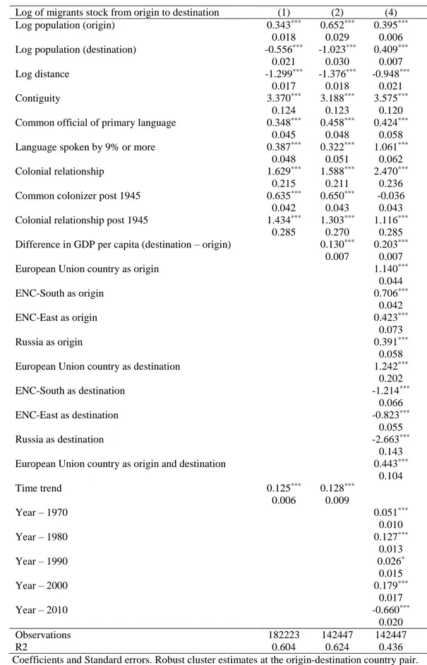
The model has been estimated with standard errors clustered for each origin and destination country combination to take into account potential heteroscedasticity and autocorrelation. The results of estimating the gravity model are shown in table 6. The first column shows the results of estimating a model in which demographic, geographic, and social/historical determinants of bilateral migration stocks are included but GDP differences between origin and destination country are not considered. As we can see from this column, all coefficients are statistically significant at the usual levels and have the expected sign. Population in origin

countries has positive and significant effects on immigrant stocks, while population in destination countries has a negative sign that is usually interpreted as limitations to migration due to capacity constraints. Immigrant stock decreases with distance and contiguity are clearly relevant. Regarding other variables, ceteris paribus, having a common language or a colonial relationship significantly increases the stock of immigrants, with the exception of a common colonizer post 1945 that has a negative effect. In sum, our results are in line with those found by previous studies and are very similar to those obtained by recent studies such as Mayda (2010), Kim and Cohen (2010) Grogger and Hanson (2011), Ortega and Peri (2013), and Llull (2013).

In model (2) of table 6, GDP per capita differences between origin and destination countries3 _{are presented. While the results for nearly all of the previous controls are quite similar}

to those shown in (1), the stock of migrants is positively associated with relative differences in GDP per capita. This result shows that better economic opportunities positively affect migration.

In order to have a better description of migration patterns from and to ENC countries, in model (3) of table 6 origin and destination country fixed effects are replaced by dummies representing different groups of countries. In particular, origin and destination countries are grouped into five categories: EU, ENC-East, ENC-South, Russia, and the rest of the world that will be used as the reference category. The results show that the EU has received and sent more immigrants in the considered period than the rest of the world even after controlling for demographic, geographical, cultural/historical, and economic variables. ENC-East, ENC-South, and Russia have also sent more immigrants than the rest of the world, but they have received significantly less. In this model, the trend has also been replace by time fixed effects. The coefficients associated with the year dummies also provide some interesting results. In particular, after controlling for the effect of demographic, geographical, and social/historical characteristics, migration stocks have significantly increased when compared to the 1960s. These results are similar to those found by Massey (1999) and Kim and Cohen (2010). However, the economic crisis has deeply affected international migration (Tilly, 2011): the value of the coefficient associated with the 2010 dummy is positive and significant, but its value is similar to that estimated for the 1980 dummy.

3 _{To check for multicollinearity among some independent variables, we calculate variance inflation factors}

(VIFs) for all the independent variables in model (2) of table 6. The mean VIF for all variables in the model was 1.61 with a maximum of 2.78 for the common language dummy and a minimum of 1.01 for GDP differences between destination and origin.

Table 6. Gravity model estimates

Log of migrants stock from origin to destination (1) (2) (4) Log population (origin) 0.343*** _0.652*** _0.395***

0.018 0.029 0.006 Log population (destination) -0.556*** _-1.023*** _0.409***

0.021 0.030 0.007 Log distance -1.299*** _-1.376*** _-0.948***

0.017 0.018 0.021 Contiguity 3.370*** _3.188*** _3.575***

0.124 0.123 0.120 Common official of primary language 0.348*** _0.458*** _0.424***

0.045 0.048 0.058 Language spoken by 9% or more 0.387*** _0.322*** _1.061***

0.048 0.051 0.062 Colonial relationship 1.629*** _1.588*** _2.470***

0.215 0.211 0.236 Common colonizer post 1945 0.635*** _0.650*** _-0.036

0.042 0.043 0.043 Colonial relationship post 1945 1.434*** _1.303*** _1.116***

0.285 0.270 0.285 Difference in GDP per capita (destination – origin) 0.130*** _0.203***

0.007 0.007 European Union country as origin 1.140***

0.044 ENC-South as origin 0.706*** 0.042 ENC-East as origin 0.423*** 0.073 Russia as origin 0.391*** 0.058 European Union country as destination 1.242***

0.202 ENC-South as destination -1.214*** 0.066 ENC-East as destination -0.823*** 0.055 Russia as destination -2.663*** 0.143 European Union country as origin and destination 0.443***

0.104 Time trend 0.125*** _0.128*** 0.006 0.009 Year – 1970 0.051*** 0.010 Year – 1980 0.127*** 0.013 Year – 1990 0.026* 0.015 Year – 2000 0.179*** 0.017 Year – 2010 -0.660*** 0.020 Observations 182223 142447 142447 R2 0.604 0.624 0.436

Coefficients and Standard errors. Robust cluster estimates at the origin-destination country pair. Models (1) and (2) also include origin country fixed effects and destination country fixed effects.

Using model (2) of table 6 we have carried out a forecasting exercise in order to obtain estimates of future migration flows.4 _{Future values for time-varying exogenous variables}

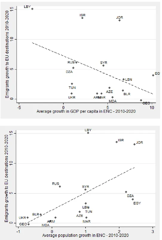
(population and GDP) are obtained from the IMF World Economic Outlook database (October 2015). The result of the forecasting exercise for bilateral migration stocks in 2020 is a 183x183-183 matrix that is available from the authors on request. In table 7 we only reproduce the forecasted values of immigrants from ENC to the EU in 2020 together with historical values for 2010. The values for the scenarios on population and GDP for the considered countries are shown in annex 3. From this table, we can see that migration from ENC countries to the EU will remain relatively stable with higher increases from ENC-South and Russia. Figure 3 shows the relationship between the obtained forecasts of migration flows from ENC to the EU and the main drivers of the obtained forecasts: average growth in GDP per capita and population growth during the forecast horizon (2010-2020). From this figure, it is very clear that there is high country heterogeneity in the forecast, but we can observe that in countries with better economic prospects and lower demographic pressures migration flows to the EU are expected to be lower than in other countries. For instance, the four countries where migration flows to the EU are supposed to increase are Israel, Jordan and Libya. We can see that in these three countries, expected population growth is among the highest (the only exceptions are Egypt and Algeria) and GDP growth is not among the highest. Last, it is worth mentioning that the forecasting exercise does not consider the potential variation in other push and pull factors apart of those related to our gravity model specification. Our current analysis only provides an assessment of potential migration flows from ENC to the EU based on economic drivers and assuming that there will be no further deterioration/improvement of migration policies or in the political stability in origin countries. However, and as shown in table 5, several additional variables are not controlled here that can exert an important influence on migration flows, as we have recently seen during the 2015 refugee crisis in Europe.

4 _{The forecasting performance of the model has been assessed using the Stavins and Jaffe (1990) goodness}

of fit statistic as in Burger et al. (2009) and Martínez-Zarzoso (2013). The obtained values for models in table 6 are 0.72, 0.76 and 0.72, respectively. The same statistic has been calculated for the Poisson Maximum likelihood estimates yielding similar values: 0.71, 0.75 and 0.61. Moreover, for non-zero origin-destination pairs for the time periods considered we have calculated the in-sample 1-period ahead Mean Absolute Percentage Error (MAPE). The values obtained for the OLS estimates are 2.5%, 2.1% and 2.1%, while for the Poisson estimates are significantly higher: 16.2%, 15.4% and 45%, respectively. The values of the ex-post 1-period ahead MAPE for model (2) in table 6 also indicate a good forecasting performance of the model: a 4.53% on average (with a minimum value 2.47% in 1970 and a maximum value of 6.18% in 2010).

Table 7. Forecasting exercise: Stock of emigrants to EU destinations Country of origin 2010 2019 2010-2019 Armenia 65,899 66,491 0.90% Azerbaijan 36,103 36,780 1.88% Belarus 218,604 221,751 1.44% Georgia 95,997 95,827 -0.18% Moldova 187,310 187,860 0.29% Ukraine 1,030,697 1,040,206 0.92% Total ENC- East 1,634,610 1,648,916 0.88%

Algeria 1,078,191 1,133,980 5.17% Egypt 219,253 227,916 3.95% Israel 63,193 71,726 13.50% Jordan 34,407 38,925 13.13% Lebanon 195,117 201,493 3.27% Libya 27,836 32,030 15.07% Morocco 2,575,993 2,599,498 0.91% Syria 129,390 136,596 5.57% Tunisia 492,597 505,303 2.58% Total ENC-South 4,815,977 4,947,466 2.73% Total ENC 6,450,587 6,596,381 2.26% Russia 1,096,687 1,163,891 6.13% Total ENC + Russia 7,547,274 7,760,272 2.82%

Figure 3. Change in the stock of emigrants to EU destinations from ENC and average growth in GDP per capita in ENC (top panel) and

average population growth in ENC (bottom panel) 2010-2020

Note: ARM: Armenia; AZE: Azerbaijan; BLR: Belarus; GEO: Georgia; MDA: Moldova; UKR: Ukraine; DZA: Algeria; EGY: Egypt; ISR: Israel; JOR: Jordan; LBN: Lebanon; LBY: Libya; MAR: Morocco; SYR: Syria; TUN: Tunisia; RUS: Russia.

FINAL REMARKS

The objective of this paper is to analyse past and future migration trends between ENC and the EU. We have provided empirical evidence on population and migration trends in ENC, and we have specified and estimated a gravity model covering around 200 countries and have used the model to obtain medium-run migration forecasts from ENC to the EU.

The descriptive analysis of population and migration trends in ENC countries has shown some interesting results. First, the population of the ENC has increased by 170 million people between 1960 and 2010 while the EU-29 has increased its population only by 100 million. Second, there is a very high heterogeneity regarding migration trends in ENC countries in the last 50 years. While some countries, such as Israel during the whole period or Russia over the last 30 years, have been net migration receivers, other countries, such as Belarus, Egypt, or Tunisia have clearly lost population due to migration. Third, migration from ENC countries is highly concentrated in some destination countries due to geographical proximity or strong political, economic, or colonialist linkages.

Our analysis of the long-run determinants of bilateral migration stocks has permitted us to conclude that demographic, geographical, social/historical, and economic factors are relevant both to explain and to forecast migration patterns. Our results have shown that once pull and push factors are controlled, migratory movements from ENC countries to the rest of the world are higher than they should be according to the model. When we concentrate on migrants from ECN to the EU, this “surplus” is even higher. This result shows the strong ties between these countries and the EU and that migration from the ENC can clearly increase migratory pressure in the future. In fact, our medium-run forecasts show an increase in migration from ENC countries to the EU will at around 200,000 migrants (2.8%), with higher increases from ENC-South and Russia. It is worth mentioning that there is a high heterogeneity in the forecast at the country level.. It is also important to highlight that our analysis is focused on economic migrants and refugees and asylum seekers are not considered in our forecasting exercise. However, as we have recently seen in the 2015-2016 refugee crisis in Europe, these movements can be very relevant but its drivers (such as armed conflicts or natural disasters) are extremely difficult to predict. Nonetheless, these flows are usually less persistent as drivers tend to be short-term and one-off events. In any case, as Neumayer (2005) highlights “persistent episodes of conflict and violence can increase economic hardship in countries of origin” and, as a result, in this context it is difficult to separate non-economic determinants of migration from non-economic ones in the medium run. In fact, there are additional pull and push factors of migration (in a broad sense) that our forecasting exercise is not considering and that can exert an important influence on people flows.

Regarding future directions for research, the availability of the compiled dataset on bilateral migration stocks and several determinants can serve as a starting point to enlarge our benchmark specification to include other variables that are potentially interesting in the context of the ENP. For instance, indicators on quality of governance or other institutional determinants could be included as additional explanatory variables, and different scenarios regarding institutional convergence with the EU could be considered in order to assess the future evolution of migration from and to ENC.

REFERENCES

Bertoli, S., Fernandez-Huertas Moraga, J: (2013), “Multilateral Resistance to Migration”, Journal

of Development Economics, 102, pp. 79-100.

Brücker, H., Siliverstovs, B. (2006), “On the estimation and forecasting of international migration: How relevant is heterogeneity across countries?”, Empirical Economics, 31 (3), pp. 735-754. Burger, M., van Oort, F., Linders, G. (2009), “On the Specification of the Gravity Model of Trade: Zeros, Excess Zeros and Zero-inflated Estimation”, Spatial Economic Analysis, 4 (2), pp. 167-190.

Crespo-Cuaresmo, J., Moser, M. Raggl, A. (2013), “On the Determinants of Global Bilateral Migration Flows”, WWWForEurope, Working Paper no 5.

Fertig, M., Schmidt, C. M. (2000), Aggregate-level migration studies as a tool for forecasting future migration streams, IZA Discussion Paper 183.

Gallardo-Sejas, H., Gil Pareja, S., Llorca-Vivero, R., Martínez-Serrano, J. A. (2006), “Determinants of European immigration: a cross-country analysis”, Applied Economics Letters, 13 (12), pp. 769-773.

Grogger, J., Hanson, G. H. (2011), “Income maximization and the selection and sorting of international migrants”, Journal of Development Economics, 95 (1), pp. 42–57

Hatton, T., Williamson, J. G. (2002), What fundamentals drive world migration?, NBER Working Paper no. 9159

Head, K., Mayer, T., Ries, J. (2010), “The erosion of colonial trade linkages after independence”,

Journal of International Economics, 81(1), pp. 1-14.

Head, K., Mayer, T. (2013), "Gravity Equations: Toolkit, Cookbook, Workhorse", in Handbook of International Economics, Vol. 4,eds. Gopinath, Helpman, and Rogoff, Elsevier.

Karemera, D., Oguledo, V.I., Davis, B. (2000), “A gravity model analysis of international migration to North America”, Applied Economics, 32 (13), pp. 1745-1755.

Kim, K., Cohen, J.E. (2010), “Determinants of international migration flows to and from industrialized countries: A panel data approach beyond gravity”, International Migration Review, 44 (4), pp. 899-932.

Llull, J. (2013), “Understanding International Migration: Evidence from a New Dataset of Bilateral Stocks (1960-2000)”, Barcelona GSE Working Paper 715.

Martínez-Zarzoso, I. (2013), “The log of gravity revisited”, Applied Economics, 45 (3), pp. 311-327.

Massey, D. S. (1999), “International Migration at the Dawn of the Twenty-First Century: The Role of the State”, Population and Development Review, 25 (2), pp. 303–322.

Mayda, A. M. (2010), “International migration: a panel data analysis of the determinants of bilateral flows”, Journal of Population Economics, 23 (4), pp. 1249-1274.

Neumayer, E. (2005), “Bogus Refugees? The Determinants of Asylum Migration to Western Europe”, International Studies Quarterly, 49 (3), pp. 389-409.

Ortega, F., Peri, G. (2009), “The Causes and Effects of International Migrations: Evidence from OECD Countries, 1980–2005”, NBER Working Paper No. 14833.

Ortega, F., Peri, G. (2013). “The effect of income and immigration policies on international migration”, Migration Studies, 1 (1), pp. 47-74.

Özden, Ç., Parsons, C., Schiff, M., Walmsley, T. L. (2011), “Where on Earth is Everybody? The Evolution of Global Bilateral Migration, 1960-2000”, World Bank Economic Review, 25 (1), pp. 12-56.

Praussello, F. (2011), “The European Neighbourhood Policy and migration flows”, mimeo

Santos Silva, J. M. C., Tenreyro, S. (2006), “The log of gravity”, Review of Economics and

Statistics, 88, pp. 641–658.

Stavins, R. N., Jaffe, A. B. (1990), “Unintended Impacts of Public Investments on Private Decisions: The Depletion of Forested Wetlands”, American Economic Review, 80, pp. 337-352. Tilly, C. (2011), “The impact of the economic crisis on international migration: A review”, Work,

Employment and Society, 25 (4), pp. 675-692

Volger, M., Rotte, R. (2000), “The effects of development on migration: theoretical issues and new empirical evidence”, Journal of Population Economics, 13, 485–508.

Annex 1. Datasets description

Data set Countries and periods Description World Bank Bilateral Migration Database 1960-2000

World Bank Bilateral Migration Matrix 2010

226 countries 1960, 1970, 1980, 1990, 2000, 2010

Bilateral migration stocks

http://data.worldbank.org/data-catalog/global-bilateral-migration-database http://go.worldbank.org/JITC7NYTT0

CEPII Geodist dataset and gravity data 225 countries 1960-2006

GeoDist 's provides several geographical variables, in particular bilateral distances measured using city-level data to assess the geographic distribution of population inside each nation. The dyadic file includes a set of different distance and common dummy variables used in gravity equations to identify particular links between countries such as colonial past, common languages or contiguity. The gravity dataset also includes information on additional time-varying variables usually included in gravity models such as GDP.

http://www.cepii.fr/anglaisgraph/bdd/distances.htm http://www.cepii.fr/CEPII/en/bdd_modele/presentation.asp

Annex 2. Gravity model estimates using a Poisson model

Migrants stock from origin to destination (1) (2) (3) Log population (origin) 1.398*** _1.429*** _0.615***

0.136 0.163 0.018 Log population (destination) 0.136 -0.022 0.776***

0.112 0.149 0.020 Log distance -1.313*** _-1.276*** _-0.958***

0.036 0.036 0.046 Contiguity 0.843*** _0.858*** _1.182***

0.065 0.068 0.134 Common official of primary language 0.110 0.078 -0.017 0.088 0.091 0.137 Language spoken by 9% or more 0.717*** _0.752*** _1.018***

0.087 0.092 0.138 Colonial relationship 0.989*** _1.061*** _1.020***

0.113 0.113 0.122 Common colonizer post 1945 1.496*** _1.454*** _0.328**

0.089 0.094 0.154 Colonial relationship post 1945 1.487*** _1.368*** _0.935***

0.132 0.133 0.131 Difference in GDP per capita (destination – origin) 0.089** _0.499***

0.043 0.015 European Union country as origin 1.489***

0.096 ENC-South as origin -0.696*** 0.100 ENC-East as origin 0.931*** 0.131 Russia as origin 0.277*** 0.103 European Union country as destination 1.452***

0.144 ENC-South as destination 0.144 0.170 ENC-East as destination -0.809*** 0.112 Russia as destination -0.394** 0.164 European Union country as origin and destination -0.298**

0.146 Time trend -0.004 0.011 0.019 0.027 Year – 1970 -0.116 0.125 Year – 1980 -0.114 0.118 Year – 1990 -0.185* 0.112 Year – 2000 -0.205* 0.121 Year – 2010 -0.125 0.121 Observations 182223 142447 142447 Pseudo-R2 0.778 0.759 0.377

Coefficients and Standard errors. Models (1) and (2) also include origin country fixed effects and destination country fixed effects.

Annex 3. Scenarios on population and GDP growth for ENC

Average annual growth rates 2010-2020 Population GDPpc

Armenia 0.2% 5.7% Azerbaijan 0.9% 10.9% Belarus -0.4% 10.4% Georgia -0.1% 11.9% Moldova 0.0% 9.0% Ukraine -0.2% 5.2%

Total ENC- East -0.1% 7.9%

Algeria 2.0% 5.1% Egypt 2.4% 11.1% Israel 2.4% 4.3% Jordan 2.5% 6.7% Lebanon 1.0% 6.5% Libya 1.2% 4.7% Morocco 1.0% 7.3% Syria 1.6% 4.5% Tunisia 1.1% 2.1% Total ENC-South 1.9% 6.5% Total ENC 1.3% 6.9% Russia 0.1% 7.7%

Total ENC + Russia 0.9% 6.9% Source: IMF World Economic Outlook Database October 2015