Vol. 1, No. 1 (2007) 1–17 c
World Scientific Publishing Company
PERMUTATION DISALIGNMENT INDEX AS AN INDIRECT,
EEG-BASED, MEASURE OF BRAIN CONNECTIVITY
IN MCI AND AD PATIENTS
NADIA MAMMONE, LILLA BONANNO, SIMONA DE SALVO, SILVIA MARINO, PLACIDO BRAMANTI
IRCCS Centro Neurolesi Bonino-Pulejo
Via Palermo c/da Casazza, SS. 113, 98124 Messina, Italy [email protected], [email protected]
ALESSIA BRAMANTI
Institute of Applied Sciences and Intelligent Systems Eduardo Caianiello (ISASI) National Research Council (CNR), Messina (Italy)
FRANCESCO C. MORABITO
DICEAM Department of the Mediterranea University of Reggio Calabria Via Graziella Feo di Vito, 89060 Reggio Calabria, Italy [email protected]
Received Day Month Year Revised Day Month Year
OBJECTIVE: In this work, we introduce Permutation Disalignment Index (PDI) as a novel nonlinear, amplitude independent, robust to noise metric of coupling strength between time series, with the aim of applying it to electroencephalographic (EEG) signals recorded longitudinally from Alzheimer’s Disease (AD) and Mild Cognitive Impaired (MCI) patients. The goal is to indirectly estimate the connectivity between the cortical areas, through the quantification of the coupling strength between the corresponding EEG signals, in order to find a possible matching with the disease’s progression. METHOD: PDI is first defined and tested on simulated interacting dynamic systems. PDI is then applied to real EEG recorded from 8 amnestic MCI subjects and 7 AD patients, who were longitudinally evaluated at time T0 and 3 months later (time T1). At time T1, 5 out of 8 MCI patients were still diagnosed MCI (stable MCI), whereas the remaining 3 exhibited a conversion from MCI to AD (prodromal AD). PDI was compared to the Spectral Coherence and the Dissimilarity Index. RESULTS: Limited to the size of the analysed dataset, both Coherence and PDI resulted sensitive to the conversion from MCI to AD, even though only PDI resulted specific. In particular, the intrasubject variability study showed that the three patients who converted to AD exhibited a significantly (p < 0.001) increased PDI (reduced coupling strength) in delta and theta bands. As regards Coherence, even though it significantly decreased in the three converted patients, in delta and theta bands, such a behaviour was detectable also in one stable MCI patient, in delta band, thus making Coherence not specific. From the Dissimilarity Index point of view, the converted MCI showed no peculiar behaviour. CONCLUSIONS: PDI significantly increased, in delta and theta bands, specifically in the MCI subjects who converted to AD. The increase of PDI reflects a reduced coupling strength among the brain areas, which is consistent with the expected connectivity reduction associated to AD progression.
Keywords: Electroencephalography, Alzheimer’s Disease, Mild Cognitive Impairment, Permutation Dis-alignment Index.
February 15, 2017 10:20 WSPC/INSTRUCTION FILE paper˙PDI˙MCI˙AD˙IJNS˙v3
2 N. Mammone, L. Bonanno, S. De Salvo, S. Marino, P. Bramanti, A. Bramanti, Francesco C. Morabito
1. Introduction
Dementia is a general term used to refer to a wide range of symptoms, associated with a decline in memory or other thinking skills, which reduce a person’s ability to perform everyday life activities. Alzheimer’s disease (AD) is the most common form of dementia and ac-counts for 60% of dementia cases1. Current diagnosis of AD relies on quantifying the mental decline. How-ever, by the time the patient is diagnosed, the disorder has already caused severe brain damage. Studies suggest that AD begins years before the clinical symptoms be-come visible2. Furthermore, normal ageing is also char-acterised by a slow decline of cognitive functions, thus discriminating normal ageing from AD, at a very early stage, can be challenging when relying only on standard procedures based on clinical evaluation.
Researchers hope to develop an accurate way to early detect AD before its devastating symptoms appear. To this purpose, high-risk population should be periodi-cally monitored through an early detection system. With regard to high-risk population, Mild Cognitive Impair-ment (MCI) is a condition in which the subject experi-ences minor problems with cognition (memory or think-ing) and involves nearly 5-20% of people aged over 65. In MCI patients, cognitive issues are worse than we nor-mally expect for a healthy person of the same age, but the symptoms are not severe enough to interfere signif-icantly with daily life, thus, MCI is not labelled as de-mentia2. In recent clinical studies, amnestic MCI sub-jects were shown to have an increased risk of develop-ing AD. The incidence of AD, observed in 4 studies on amnestic MCI, ranged from 10.2% to 26.0% (median: 17.6%) over 1 year and from 17.6% to 36.3% (median: 24.2%) over 2 years3. Therefore, this population should be studied on the long term and longitudinally, in order to develop a system that can help to predict the transition from MCI to AD. Such a system should necessarily be non-invasive, well tolerated and low-cost; thus it could be based on Electroencephalography (EEG). The EEG consists in recording the electrical potentials generated by the brain through a set of electrodes located on the scalp. In AD patients, EEG abnormalities arise because of anatomical and functional deficits of the cerebral cor-tex. One of the effects of such deficits is the functional disconnection between some cortical areas: such a dis-connection affects the behaviour of the electrical activity of the brain and, therefore, alter the EEG4.
Adeli et al. presented an overview of computational modelling for the analysis of EEGs recorded from AD patients5 6. The hallmarks of EEG abnormality in AD patients, compared to healthy controls, are often a shift
of the power spectrum to lower frequencies and reduced coherences among cortical regions7, which are thought to be associated with functional disconnections among cortical areas resulting from the death of cortical neu-rons8. An EEG-based diagnostic tool should reveal the effects of such disconnection over the scalp; to this pur-pose, the mapping of descriptive features 9, 10, 11, 12, might help. Stam et al. proposed to compute the syn-chronisation likelihood of multichannel EEG data in AD patients, subjects with MCI and subjects with subjec-tive memory complaints (SC). The synchronisation like-lihood significantly decreased in the 14-18 and 18-22 Hz bands in AD patients compared with both MCI subjects and healthy controls13.
Dunkin et al. hypothesised that decreased coher-ence would be associated with cognitive dysfunction as assessed by neuropsychological tests. They found that reduced coherence was associated with impairment on specific neuropsychological tests. The results en-dorsed the hypothesis that coherence reflects a func-tional breakdown in communication between brain ar-eas14. Sankari et al.15presented a comprehensive study of intrahemispheric, interhemispheric and distal EEG coherence in AD patients. Their study showed a pattern of decrease in AD coherence, by indicating a decline in cortical connectivity but they also report exceptions in specific bands where an increase in coherence can be at-tributed to compensatory mechanisms. Adeli et al. pre-sented a wavelet coherence investigation of EEG read-ings acquired from patients with AD and healthy con-trols. Pairwise electrode coherence and wavelet coher-ence were calculated over each frequency band (delta, theta, alpha, and beta)16,17.
High EEG upper/low alpha power ratio was asso-ciated with cortical thinning and lower perfusion in the temporo-parietal lobe. Moreover, atrophy and lower per-fusion rate were both significantly correlated with mem-ory impairment in MCI subjects 18. In 19, correlation between EEG markers and volumetric differences in mapped hippocampal regions was estimated in AD pa-tients. Results showed that the increase of alpha3/alpha2 power ratio is correlated with atrophy of mapped hip-pocampal regions in AD. In 20, the most significant results of recent studies on correlation between scalp EEG, cognitive decline, and anatomical substrate have been reviewed, with particular attention to the relation-ships between EEG changes and hippocampal atrophy.
Morabito et al. 4 proposed a technique, based on Complex Networks, to analyse the longitudinal mod-ifications of brain connectivity and information trans-fer in AD patients. They found out that the
progres-sion of AD was characterised by a loss of connected areas, in terms of network parameters. Since the evo-lution of AD is characterised by the progressive loss of functional connectivity within neocortical associa-tion areas, Giannakopoulos et al. supposed that event-modulated EEG dynamic analysis could allow to inves-tigate the functional activation of neocortical circuits. They reviewed and summarised clinically significant re-sults of EEG activation studies in this field and dis-cussed future perspectives of researches which aim at reaching an early and individual prediction of cogni-tive decline in healthy elderly controls 21. Prichep et al. reported results from initial quantitative electroen-cephalography (qEEG) evaluations of normal elderly subjects. Source localisation algorithms were used to identify the most probable generators of abnormal fea-tures in the EEG. Abnormalities were found in the pro-dromal EEGs of those subjects who later converted to dementia22. Rossini et al. analysed the cortical connec-tivity (spectral coherence) and the low resolution brain electromagnetic tomography sources of EEG rhythms in MCI patients at baseline and follow-up 23. They found out that low midline coherence and weak tem-poral source were associated with a 10% annual rate of MCI to AD conversion. The National Institute on Aging and the Alzheimer’s Association (NIA/AA) workgroup of experts postulated that what is commonly considered Alzheimer should rather be considered a mere stage of a long, complex degenerating process24and, therefore, they strongly encouraged the researchers to engage lon-gitudinal studies. However, the literature lacks longitu-dinal studies on MCI/AD, because keeping such patients and their caregivers loyal to a periodical follow-up pro-gram can be challenging.
To our best knowledge, and also according to the review paper 25, the most promising work about MCI conversion to AD is26, they reported that IFAST method was able to predict the conversion from amnestic MCI to AD with high accuracy (85.98%) in a 1-year follow-up study. This methodology was later improved but it has been validated only in a MCI vs AD vs Controls cross study so far 27. As already claimed above, MCI and AD are known as disconnection disorders, because it is well accepted that MCI/AD weakens the connectivity between the areas of the brain. Changes in the connec-tivity between cortical areas are likely to induce changes in the coupling strength between the corresponding EEG signals, this is the reason why a measure of coupling strength between EEG signals might help to indirectly estimate the changes in the brain connectivity due the disease’s progression. The present work resulted from a
translational research whose goal was to longitudinally evaluate the evolution of the brain connectivity in MCI and AD patients, indirectly, through the EEG. The spe-cific aim was to compare the overall coupling strength between EEG signals at time T0 and at time T1, in MCI and AD patients, in order to assess if it could reflect the brain connectivity reduction that is expected to be induced by the disease’s progression. Our first evalua-tion was carried out applying Spectral Coherence be-cause it is the gold standard method for the indirect estimation of the brain connectivity from the EEGs of AD and MCI patients. The reason for that is Coherence-based analysis comes with most of the EEG process-ing systems used in clinical applications on MCI/AD
27. As Coherence showed a trend that was peculiar to
converted MCI but also exhibited a false positive, even though our dataset was small, we decided to develop our own metric for the estimation of coupling strength be-tween time series. We introduced the Permutation Dis-alignment Index (PDI), which is a novel measure of coupling between time series, that can help whenever a multivariate, amplitude invariant, robust to noise, non-linear coupling strength analysis is necessary. With ap-plication to EEG signals, PDI can be interpreted as an indirect measure of the coupling strength between two or more cortical areas, estimated through the quantifi-cation of the alignment randomness between the cor-responding EEG projected time series. From the theo-retical point of view, we can address the advantages of analysing the EEG through PDI, as compared to Coher-ence, to endorse our choice to develop a novel, nonlin-ear, multivariate, symbolic coupling strength descriptor: 1) Coherence is not a multivariate but only a pairwise descriptor, thus it cannot be exploited to estimate the joint coherence of a group of electrodes, on the contrary, PDI can be both multivariate and pairwise thus it can be exploited to estimate the coupling strength between a pair of electrode sites or among a group of electrodes covering a more extended area; 2) Coherence is linear and can fail to capture the nonlinear dynamics of the EEG; 3) Coherence is not a symbolic methodology and can be more sensitive to noise, since our method relies on the projection onto a predetermined set of symbols (the motifs), the possible presence of amplitude burst in the EEG due to artifacts would not cause amplitude burst in the projected symbols, therefore in the descrip-tor. Considered such motivations, PDI was hereby de-fined, implemented and, first of all, tested on simulated unidirectionally coupled Henon maps, in order to vali-date PDI’s ability to measure the coupling strength be-tween interacting dynamic systems. Since PDI
success-February 15, 2017 10:20 WSPC/INSTRUCTION FILE paper˙PDI˙MCI˙AD˙IJNS˙v3
4 N. Mammone, L. Bonanno, S. De Salvo, S. Marino, P. Bramanti, A. Bramanti, Francesco C. Morabito fully reflected the coupling stregth variations in the
sim-ulated coupled systems, it was tested on real EEG sig-nals recorded during a follow-up study which involved 7 AD patients and 8 amnestic MCI patients. The patients were evaluated at time T0 and then, 3 months later, at time T1.
Besides Coherence, PDI was also compared to the Dis-similarity Index (Dm) proposed by Ouyang et al. 28, which is a nonlinear, symbolic dissimilarity measure between time series that, in our opinion, was the best-matching nonlinear method.
According to the achieved results, PDI seems to have a high potential in the analysis of MCI/AD EEG time series. We hope that the present work encour-ages longitudinal studies on MCI patients, which are of paramount importance in the prediction of the degener-ation from MCI to AD.
The paper is organised as follows: Section 2 de-scribes how the patients were selected and how the EEGs were recorded and preprocessed. Section 3 in-troduces the concept of PDI and describe how it was tested on simulated data and on the experimental EEG data. Section 5.3 introduces the standard comparative methodologies used in the quantitative EEG analysis (spectral coherence and dissimilarity index). Section 6 reports the achieved results, Section 7 discusses the re-sults and Section 8 addresses the conclusions.
2. EEG data recording and preprocessing 2.1. Study population
Fifteen patients, 7 AD subjects and 8 MCI subjects, at various stages of clinical evolution, were recruited at the IRCCS Centro Neurolesi Bonino-Pulejo of Messina (Italy). All patients were enrolled within an ongoing co-operation agreement that also included a clinical proto-col approved by the local Ethical Committee. All pa-tients signed an informed consent form. The clinical di-agnosis was performed, according to the Diagnostic and Statistical Manual of Mental Disorders (fifth edition, DSM-5)29, by a multidisciplinary team including neu-rologists, psychologists, psychiatrists and EEG experts, through a complete medical assessment. The same ex-aminers conducted all the cognitive and clinical evalu-ations. Every patient underwent a neuroradiological ex-amination to exclude other conditions (tumors, strokes, damage from severe head trauma or buildup of fluid in the brain, etc) that may cause symptoms similar to AD but require different treatment. Current use of any medications (but particularly cholinesterase inhibitors (ChEis), Memantine, anti-depressants, anti-psychotics and anti-epileptic drugs) was also taken into account
in AD patients. MCI patients were not undergoing any medical treatment. All patients were assessed at baseline (time T0) and 3 months after the first evaluation (time T1). At time T1, 3 MCI patients exhibited a conversion from MCI to AD. Table I provides details about gender (Female/Male), age and diagnosis (MCI or AD) of every patient.
2.2. EEG recording
The EEG was recorded in a comfortable resting state, according to the 10-20 International System (19 chan-nels: Fp1, Fp2, F3, F4, C3, C4, P3, P4, O1, O2, F7, F8, T3, T4, T5, T6, Fz, Cz and Pz), at a sampling rate of 1024 Hz, by using a notch filter at 50Hz, with linked earlobe (A1-A2) reference. Before the EEG record-ing, all patients and their caregivers underwent a semi-structured interview including questions about: (a) qual-ity of the last night sleep; (b) duration of the last night sleep; (c) meal timing and content. The EEG recordings were performed in the morning. During the acquisition of the EEG, the patients kept their eyes closed but re-mained awake. The technician, keeping the subject alert by calling her/him name, prevented the drowsiness: the corresponding EEG segments were discarded to avoid the effects of auditory cortex activation. The patients did not sleep during the recording as confirmed by the EEG recordings which did not show any sleep pattern. The EEG was initially sampled ad 1024Hz, according to the general EEG recording protocol adopted at the IRCCS Neurolesi Center. The sampling rate was set high in or-der to make the EEG dataset as general as possible, in order to be suitable also for possible future researches with different goals.
2.3. EEG preprocessing
EEG signals are commonly decomposed into the four major EEG sub-bands: delta (0-4 Hz), theta (4-8 Hz), alpha (8-12 Hz), and beta (12-32 Hz). Each of the four sub-bands relates to different functional and physiological parts of the brain. In this paper, the EEG was band-pass filtered at 0.1-32Hz, then it was split into the four sub-bands through a set of band-pass filters implemented in the toolbox EEGLab (https://sccn.ucsd.edu/eeglab/)30. In particular, we used the function eegfiltfft, based on Fast Fourier Transform (FFT) and inverse FFT to reconstruct only the specific frequency range under consideration. Figure 1 shows an EEG signal (filtered between 0.1 and 32 Hz) and the corresponding sub-bands. Starting from one n-channels EEG recording, we eventually end up with 4 different n-channels EEG recordings, each one corresponding to a different frequency sub-band: EEGδ, EEGθ, EEGα,
EEGβ. Each sub-band-EEG was then downsampled to
256Hz. Considered the specific application, 256Hz is a sampling rate high enough to capture delta, theta, al-pha and beta waves, which are typically analysed in AD/MCI patients. 0 200 400 600 800 1000 1200 1400 1600 1800 2000 −50 0 50 EEG 0 200 400 600 800 1000 1200 1400 1600 1800 2000 −20 0 20 EEG delta 0 200 400 600 800 1000 1200 1400 1600 1800 2000 −10 0 10 EEG theta 0 200 400 600 800 1000 1200 1400 1600 1800 2000 −10 0 10 EEG alpha 0 200 400 600 800 1000 1200 1400 1600 1800 2000 −10 0 10 EEG beta Time(samples)
Fig. 1. An EEG signal (filtered between 0.1 and 32 Hz and ex-pressed in µV ), and the corresponding delta (0-4 Hz), theta (4-8 Hz), alpha (8-12 Hz), and beta (12-32 Hz) sub-bands.
Every sub-band-EEG recording was partitioned into 5 s non-overlapping windows (as the sampling rate after downsampling is 256Hz, each window included Ns = 1280 EEG samples); therefore, each sub-band-EEG was eventually partitioned into Nw non-overlapping windows, where Nw depends of the length of the record-ing. All the algorithms were implemented in Matlab
(The MathWorks, Inc., Natick, MA, USA).
Before processing the filtered EEG through the pro-posed algorithm, artifactual segments were manually la-belled by EEG experts and then cancelled. However, it is worth to point out that, since the algorithm processes the EEG window by window and then it averages the es-timated parameters over the windows, the effect of pos-sible artifacts is mitigated. The average time length of the recordings, after artifact cancellation, is 5.44min. 3. A novel, EEG-based, indirect measure
of brain connectivity: Permutation Disalignment Index
PE was introduced by Bandt and Pompe in 200231as a symbolic robust descriptor which detects dynamic com-plexity changes in time series. Thanks to the projection into symbols (motifs), PE allows to estimate the ran-domness of a time series regardless of its amplitude, which plays a key role when analysing EEG, whose am-plitude depends on the location of the reference elec-trode. In fact, when processing the EEG recordings through amplitude dependent techniques, each EEG sig-nal should be normalised to cancel the effect of close-ness to the reference electrode. Normalisation is not necessary when a symbolic procedure like PE is used. However, PE is a univariate descriptor which can only describe the randomness of a single time series (i.e. a signal recorded at a specific electrode site) and cannot quantify the coupling between two or more time series (i.e. between two or more different cortical areas). We will now briefly recall the PE definition in order to prop-erly introduce our PDI concept.
3.1. Definition of Permutation Entropy
Given a time series x with N samples, it can be mapped into a m-dimensional space, with m being the embed-ding dimension and L being the time lag. Starting from a given sample x(t) in the EEG window under analy-sis, a m-dimensional Xt vector is constructed, picking
up the remaining m − 1 samples with a L-samples shift forward:
Xt= [x(t), x(t + L), ..., x(t + (m − 1)L)]T (1)
Then the algorithm moves to the next sample x(t + 1) and reiterates the procedure, so a new vector Xt+ 1
is constructed.
The values of Xt are ordered, in increasing order
and a reshaped version Xrtof the original Xtis defined:
February 15, 2017 10:20
WSPC/INSTRUCTION FILE
paper˙PDI˙MCI˙AD˙IJNS˙v3
6 N. Mammone, L. Bonanno, S. De Salvo, S. Marino, P. Bramanti, A. Bramanti, Francesco C. Morabito With τi = 1, ..., m, where τi tells us is what
posi-tion the sample x(τi) was in the original vector Xt.
By reshaping the vectors (and then considering the original time points associated to the elements of the re-shaped vectors) we are essentially discarding the am-plitude of the components and only taking into account their relative levels. We now need to associate the ob-served pattern to a predetermined symbol (motif). The sequence of the time points will tell us what motif the observed pattern can be associated to. In other words, each vector Xt can be considered mapped onto a
sym-bol vector πi = [τ1, τ2, ..., τm] (where i=1,... m! and m!
is the number of the possible permutations); πi is a
se-quence of time points, therefore a sese-quence of integers. The occurrence rate of a given sequence πi in the time
series x is denoted as pX(πi), and represents the
prob-ability of observing the specific symbol πi in the time
series under analysis.
The algorithm counts how many times each se-quence πi appeared in the time series, then this number
is normalised by N − (m − 1)L to estimate the proba-bility of the motif: p(πi) = n(πi)/(N − (m − 1)L). PE
is finally computed as:
H(m) = −
m!
X
i=1
p(πi)log(p(πi)) (3)
Where log is the natural logarithm. The authors have recently successfully applied a new version of PE, based on the concept of Renyi’s Entropy, i.e. the Renyi’s Permutation Entropy (PEr)32, to the study the EEG of absence seizure patients 33. In particular, the random-ness of the electrical activity of each cortical area was investigated through the estimation of the randomness of the signal recorded at the corresponding EEG channel (time series x). In that work, Renyi’s theory34was intro-duced to enhance the standard definition of PE through the introduction of the parameter α (α ≥ 0):
HR(m) = − 1 1 − αlog m! X i=1 p(πi)α (4)
For α → 1, we obtain the standard PE defini-tion. High α values emphasise the super-gaussian dis-tributions whereas low α values emphasise the sub-gaussian ones. Therefore, α can tune the sensitivity to sub-gaussianity and super-gaussianity of pdf distribu-tion. In particular, higher α values (α > 4) empha-sise the super-gaussianity, whereas average alpha values (α = 2 ∼ 3) emphasise both of them.
3.2. Permutation Disalignment Index
The aim of the present work was to define a new mea-sure of coupling strength between time series and then to test it an indirect, EEG-based, measure of brain con-nectivity in AD and MCI patients. As AD and MCI are known as disconnection disorders, we considered the coupling strength between the different cortical areas rather than the activity of the single cortical area. Fur-thermore, we were interested in symbolic descriptors, to ensure the independency from the reference-electrode. Summarising, we needed a symbolic, at least bivariate, descriptor of the coupling strength between EEG time series.
Hereby we propose a symbolic measure of coupling strength, referred to as Permutation Disalignment Index (PDI). In order to properly introduce PDI, we must refer to Section 3.1.
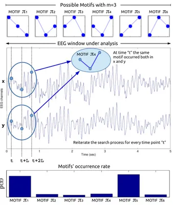
Our method is concisely illustrated in Figure 2. Let us, for example, consider m=3, for sake of clarity. When m=3, given two time series x and y, the time point t and the lag L, we can project the time series x into the vector Xt(Eq. 1) and the time series y into the vector Yt(Eq.
5):
Yt= [y(t), y(t + L), ..., y(t + (m − 1)L)]T (5)
Xtand Ytare both vectors with three elements because
m=3. The values of Xtand of Ytare reshaped in an
in-creasing order, as described in the previous Section. As explained in Section 3.1, by reshaping Xt and
Yt, and considering the original time points associated
to the elements of the reshaped vectors, we discard the amplitude of the components and we only take into ac-count their relative levels, which can be low, medium and high (when m=3). Six possible motifs can occur when m=3, in other words, six possible permutations of the low, medium and high levels (Figure 2). Given a time point t, we have to check if the same motif occurred both in x and y or not. For example, in Figure 2, at time t the same motif π4 occurred both in x and y. The procedure
is reiterated for every time point t, in this way, we even-tually come up with a final simultaneous occurrence rate pX,Y(πi) of every motif πi in x and y. Once the
occur-rence rate pX,Y(πi) of every motif has been estimated,
we can define the PDI between x and y as:
P DI(X, Y ) = 1 1 − αlog "m! X i=1 pX,Y(πi)α # (6) The more coupled x and y are, the lower the PDI is expected to be, as we expect the time series to show the same motifs with a high probability. In this work, PDI
has been defined according to the Renyi’s theory and the parameter α is introduced alongside m and L, because of the reasons discussed in Section 3.1.
p(
π)
MOTIF π1 MOTIF π2 MOTIF π3 MOTIF π4 MOTIF π5 MOTIF π6 t
EEG window under analysis
t+L t+2L
At time “t” the same motif occurred both in x and y
MOTIF π4
x
y
MOTIF π1 MOTIF π2 MOTIF π3 MOTIF π4 MOTIF π5 MOTIF π6 Possible Motifs with m=3
Reiterate the search process for every time point “t”
Motifs' occurrence rate
Fig. 2. Given two time series x and y (for example, two EEG sig-nals within an EEG window under analysis), given an embedding dimension m, a time point t and a lag L, we can project the time series x into the vector Xtand the time series y into the vector Yt,
which are both vectors with three elements. Six possible motifs (per-mutations of the low, medium and high levels) can occur when m=3. Given a time point t, the algorithm checks if the same motif occurred both in x and y or not. In the present Figure, for example, at time t the same motif π4occurred both in x and y. The procedure is
reit-erated for every time point t so that, in the end of the analysis, we come up with a final occurrence rate pX,Y(πi) of every motif πiin
xand y.
PDI can be extended to the analysis of a n-dimensional random variable X to estimate the overall coupling among all of its n components:
P DI(X1, ..., Xn) = 1 1 − αlog "m! X i=1 pX1,...,Xn(πi) α # (7) where the simultaneous occurrence of a given mo-tif πiin all of the time series X1, ..., Xnwill be
investi-gated, where i = 1, ..., m!.
3.3. Henon Maps analysis with PDI
In this work we aimed at introducing PDI as a novel measure of coupling strength between time series and
testing its ability in estimating the coupling strength be-tween real EEG signals from MCI and AD patients. First of all, we tested PDI on simulated data in order to assess its sensitivity to the changes in the coupling strength between interacting dynamic systems. The analysis of the simulated time-series yielded suggestions on the se-lection of the relevant configuration parameters for the computation of PDI. In particular, we applied PDI to the detection of nonlinear interdependency of two uni-directionally coupled Henon Maps X and Y, which have been extensively used in literature to validate measures of coupling strength35 36, they are defined as:
(
X : xn+1= 1.4 − x2n+ bxxn−1
Y : yn+1= 1.4 − [cxn+ (1 − c)yn]yn+ byyn−1
(8) System X drives system Y with a nonlinear coupling strength c, which ranges from 0 to 1 with, 0 represent-ing no couplrepresent-ing and 1 representrepresent-ing complete couplrepresent-ing. In the analysis of Identical Systems, bx is set to 0.3 and by is set to 0.3, whereas they are set to bx = 0.3 and by = 0.1 for Non Identical Systems. A detailed discus-sion about the implications of identical and nonidentical systems can be found in37.
0 0.1 0.2 0.3 0.4 0.5 0.6 0.7 0.8 0.9 1 1 2 3 4 5 Coupling strength PDI
Coupled Identical Henon Maps
alpha=1.1 alpha=2 alpha=3 alpha=4 0 0.1 0.2 0.3 0.4 0.5 0.6 0.7 0.8 0.9 1 1 2 3 4 5 Coupling strength PDI
Coupled Non Identical Henon Maps
alpha=1.1 alpha=2 alpha=3 alpha=4
Fig. 3. PDI as a function of coupling strength c and α. The top sub-plot is related to the analysis of identical Henon Maps and the bottom sub-plot is related to non-identical Henon maps.
Xand Y are initialised randomly and are iteratively computed making c increase of 0.01 every 1000 steps. A sample of PDI is computed every 1000 simulated sam-ples of X and Y. Therefore, in the range c ÷ c + 0.1, 10 PDI values are calculated because c increases with a
February 15, 2017 10:20 WSPC/INSTRUCTION FILE paper˙PDI˙MCI˙AD˙IJNS˙v3
8 N. Mammone, L. Bonanno, S. De Salvo, S. Marino, P. Bramanti, A. Bramanti, Francesco C. Morabito 0.01 increasing rate, in order to make it grow smoothly.
The ten PDI values estimated with a coupling strength ranging from a given value c to c+0.1 are then averaged and a single, average, PDI sample is associated to that c value.
In Figure 3, PDI is depicted as a function of both the coupling strength c and α, for identical (top sub-plot) and non-identical Henon maps (bottom sub-plot). PDI decreases as the coupling strength increases. This sug-gests that decreased projected alignment randomness re-flects an increased coupling strength, as expected. The behaviour is similar for different α values, even though the absolute range decreases as α increases. α=1.1 shows the widest range but a non-smooth behaviour, therefore, in this work α=2 was selected. PDI for c > 0.7 reflects a strong synchronisation between the two cou-pled systems. The critical threshold c = 0.7 corresponds to the point when the maximum Lyapunov exponent of the response system becomes negative and identical syn-chronisation between the systems takes place. For 0 < c < 0.7, PDI decreases monotonically as c increases, thus showing that PDI is sensitive even to weak coupling.
0 0.1 0.2 0.3 0.4 0.5 0.6 0.7 0.8 0.9 1 0 2 4 6 8 Coupling strength PDI
Coupled Identical Henon Maps
m=3 m=4 m=5 m=6 m=7 0 0.1 0.2 0.3 0.4 0.5 0.6 0.7 0.8 0.9 1 0 2 4 6 8 Coupling strength PDI
Coupled Non Identical Henon Maps
m=3 m=4 m=5 m=6 m=7
Fig. 4. PDI as a function of coupling strength c and embedding dimension m. The top sub-plot is related to the analysis of identi-cal Henon Maps and the bottom sub-plot is related to non-identiidenti-cal Henon maps.
Figure 4 shows PDI as a function of the coupling strength c and the embedding dimension m, for both the identical (top sub-plot) and the non-identical Henon maps (bottom sub-plot). PDI decreases as the coupling strength increases.
With regard to the identical systems, for c > 0.6, PDI increases with m, which is intuitively plausible
be-cause the projected alignment randomness of two cou-pled systems becomes inherently lower, as m increases, because the probability of observing the same symbol in the two time series is lower (in fact, the number of possible symbols is equal to m!). An abrupt change can be observed in the transition from m=6 to m=7 as the trend appears flattened both in identical and non identi-cal Systems. This suggests that, as m becomes too large, PDI becomes less sensitive to the coupling strength vari-ation. 0 0.1 0.2 0.3 0.4 0.5 0.6 0.7 0.8 0.9 1 1 2 3 4 5 6 Coupling strength PDI
Coupled Identical Henon Maps
L=1 L=2 L=3 L=4 L=5 0 0.1 0.2 0.3 0.4 0.5 0.6 0.7 0.8 0.9 1 1 2 3 4 5 6 Coupling strength PDI
Coupled Non Identical Henon Maps
L=1 L=2 L=3 L=4 L=5
Fig. 5. PDI as a function of coupling strength c and lag L. The top sub-plot is related to the analysis of identical Henon Maps and the bottom sub-plot is related to non-identical Henon maps.
A relatively high m (m > 3), would inherently re-duce the probability of a motif being detected both in signals x and y and, therefore, reduce the estimated syn-chronisation between them. In fact, as shown in 4 for the simulated Henon Maps, as m increases, the sensitivity to the coupling strength c is lost.
Furthermore, increasing m would increase the com-putational cost because the number of possible symbols, which we have to estimate the occurrence rate for, is equal to m! According to the above mentioned observa-tions, m=3 was selected in this paper.
Finally, Figure 5 shows PDI as a function of the coupling strength c and the lag L. Once again, PDI decreases as the coupling strength increases. The be-haviour looks similar for different L values. The issue of optimal selection of m and L in AD/MCI EEG was discussed in detail in 38. That paper showed that, by setting m = 3 and L = 1, the slowing effect typical of MCI/AD EEGs was better captured. Therefore, even though L = 4 looks associated to a wider range (Figure
5), since it showed the same trend as for L = 1, we se-lected L = 1. Our future work will be focused also on testing the method under different parameter settings, in order to assess how this affects the performance of the algorithm. This will be likely done on our upcoming, extended database, so that the parameter settings can be statistically optimised for MCI and AD patients. Until then, we would rely on the parameter settings m = 3 and L = 1, which was shown to work fine on AD/MCI EEG38 and also worked fine on our theoretical assess-ment on Henon Maps.
Once proven the ability of PDI to follow the vari-ation of the coupling strength between two simulated dynamical interacting systems, the next step was test-ing PDI in the quantification of the coupltest-ing strength between real systems like the electroencephalographic signals of AD and MCI patients. The goal is the indi-rect quantification of the connectivity between the corti-cal areas through the estimation of the coupling strength between the corresponding EEG signals.
4. Relative Power Analysis
As the Relative Power is a parameter commonly evalu-ated when analysing EEG from MCI and AD patients, even though it is a univariate measure and cannot di-rectly be compared to PDI, we thought that showing a Relative Power analysis over our longitudinal database was appropriate. Given an EEG window under analysis and considering the generic x-th EEG channel, the cor-responding time series is here denoted as x. The Power Spectral Density (PSD) of x is defined as the Fourier Transform of the autocorrelation function (ACF) of x:
P SDxx = F {ACFxx(t)} (9)
Once each EEG channel was band-pass filtered as described in Section 2.3, and the four sub-bands-channels were generated (xδ, xθ, xα, xβ), we can
com-pute the Relative Power (RP) of x in every sub-band (SB):
RPx=
P SD(SB)
P SD(total) (10)
which is the ratio between the PSD of the signal in the specific sub-band (f1− f2) and the overall PSD of in
the range 0.1-32Hz. The power in the sub-band f1− f2
was calculated as the integral of the PSD Pxx(f ),
es-timated between f1 and f2. In this work, the popular
Welch algorithm was used to estimate PSD39.
Given an EEGSB and given the generic window
w under analysis, the relative power RPx1,...,xkw (SB)
among the electrodes belonging to a specific scalp area (frontal, temporal, central, parietal, occipital) was calculated by averaging the EEG of the electrodes x1, ..., xk belonging to the sub-area under consider-ation and then calculating the RP over the averaged EEG. The RPx1,...,xkw (SB) values were then averaged over the windows w and a single average RP value
RPx1,...,xk(SB) was computed for every sub-area, in
every sub-band.
The average RP RPx1,...,xk(SB) values were
cal-culated both at time T0 and T1.
For every patient, the percent variation of
RPx1,...,xk(SB) (hereinafter simply denoted as RP )
was then estimated as:
4(RP (T 1)−RP (T 0))% = (RP (T 1) − RP (T 0)) RP (T 0) ∗100
(11)
5. Descriptors compared to PDI 5.1. Spectral Coherence
The magnitude squared coherence between two EEG channels x and y is defined as:
Cxy(f ) =
|Pxy(f )|2
Pxx(f )Pyy(f )
(12) where Pxy(f ) is the cross power spectral density of
xand y, Pxx(f ) and Pyy(f ) are the power spectral
den-sities of x and y, respectively. All of them are functions of the frequency f. Cxy(f ) is a function of frequency as
well, and it is a measure of synchronisation between x and y. Coherence ranges from 0 to 1, which indicates how well x corresponds to y at a given frequency f. In this work, coherence was calculated through the Welch’s averaged, modified periodogram method39.
Given the sub-band EEG recording, EEGSB, and
given the window w under analysis (w=1,..., Nw, where Nwis the number of analysed windows), the average co-herence Cx,yw (SB) between a given couple of electrodes xand y is calculated. The values Cx,yw (SB) are then av-eraged with respect to w, in order to come up with a single average Cx,y(SB) between channels x and y, for
each EEG-sub-band recording. 5.2. Dissimilarity Index (Dm)
Given an EEG segment and given a pair of EEG chan-nels (i. e. a pair of time series) x and y, they are projected into the phase space to recostruct the ordinal patterns πi,
February 15, 2017 10:20 WSPC/INSTRUCTION FILE paper˙PDI˙MCI˙AD˙IJNS˙v3
10 N. Mammone, L. Bonanno, S. De Salvo, S. Marino, P. Bramanti, A. Bramanti, Francesco C. Morabito similarly to the procedure used in PE and PDI
calcula-tion (Seccalcula-tions 3.1 and 3.2).
The occurrence rates pX(πi) and pY(πi) of each
or-dinal pattern πi on each of the two time series x and y
are calculated. After that, the distance between the rank-frequency distributions is estimated and represents the dissimilarity measure between the two time series:
Dm(X, Y ) = v u u t m! m! − 1( m! X i=1 (pX(πi) − pY(πi))2 (13) Further details can be found in Ouyang et al.28. We used the algorithm shared by Ouyang et al.through the File Exchange - MATLAB Central - MathWorkswebsite. The parameters m and L were set as for PDI.
5.3. Estimating PDI, Coherence and Dm from the EEG recordings
In order to carry out an overall scalp analysis, PDI, Co-herence and Dm, between every possible pair of
elec-trodes were computed. The aim is to evaluate the be-haviour of the above mentioned descriptors, all over the scalp, in the follow-up of MCI and AD patients (at time T0 and at time T1), in every sub-band. Consider-ing a sub-band EEGSB, obtained as described in
Sec-tion 2.3, and given a generic window w under analy-sis, the P DIx,yw (SB), the coherence Cx,yw (SB) and the Dmw
x,y(SB) between every couple of electrodes x and y
were calculated according to Sections 5.1 and 5.2. These values were then averaged over the windows (i. e. over the time) in order to come up with a single average PDI value P DIx,y(SB), a single average coherence value
Cx,y(SB) and a single average Dm value Dmx,y(SB),
for every couple, in every sub-band. For every patient, either EEG-T0 and EEG-T1, were analysed in this way. 6. Results
In this Section, we will first of all report the results of the Relative Power analysis (described in Section 4) and then we will report in detail the results of the analysis described in Section 5.
6.1. Relative Power analysis
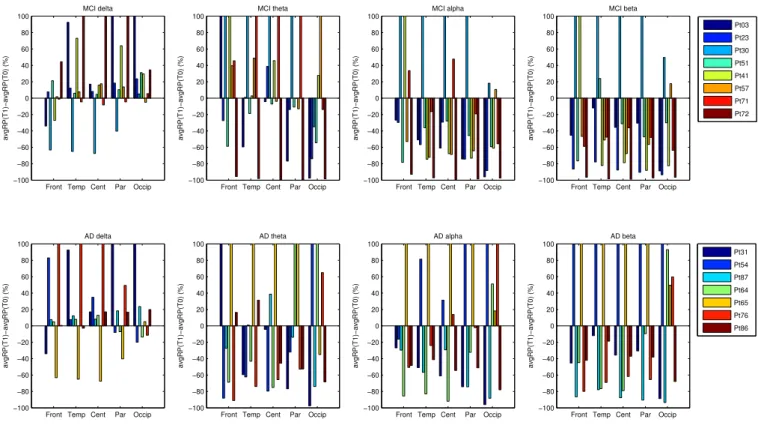
The estimated percent variations of RP (Eq. 4) are repre-sented as histograms in Figure 6. This analysis was car-ried out to detect possible shared trends in the changes of the EEG of MCI and AD patients from the point of view of RP variation. The top sub-plots, in Figure 6, are
associated to the MCI patients and the bottom ones are associated to the AD patients. Each sub-plot is associ-ated to a specific sub-band (delta, theta, alpha and beta) and the x-axis represents the scalp sub-areas (Frontal, Temporal, Central, Parietal and Occipital). Within each group, every patient is depicted with a different colour so that his/her histograms can be identified. Within each group (AD or MCI), the patients showed some common behaviour, which can be summarised as follows: • The temporal and parietal areas of MCI patients
showed decreased RP in alpha band;
• The central and parietal areas of MCI patients showed decreased RP in beta band;
• The central area of AD patients showed increased RP in delta band;
• The frontal area of AD patients showed decreased RP in alpha band.
6.2. PDI vs Coherence vs Dm analysis
The main goal of the present paper was to develop a new indirect measure of connectivity and to apply it to the EEG of MCI and AD patients in order to investigate possible correlations with the disease’s development. In other words, we aimed at finding possible EEG mark-ers that are able to discriminate between stable MCI and MCI degenerating towards AD. We decided to examine in detail the overall scalp variation of PDI levels in the transition from T0 to T1, and to compare it with Coher-ence and Dm.
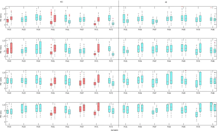
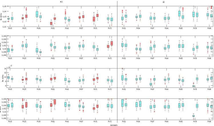
Figures 7, 8, 9 show the boxplots of PDI, Coher-ence and Dm, respectively. All of the three descriptors were estimated at time T0 and T1, according to the pro-cedure described in Section 5. Boxplots are coloured ac-cording to the results provided by the statistical analysis discussed in Section 6.3.
Every boxplot in Figure 7, shows the P DIx,y(SB)
values calculated for every couple of electrodes x and y at time T0 or T1. Given a patient under considera-tion, the boxplot on the left is associated to time T0 and the one on the right is associated to time T1. Sim-ilarly, the single boxplot in Figure 8 and 9 shows the Cx,y(SB) values (Figure 8) and the Dmx,y(SB)
val-ues (Figure 9), calculated for every couple of electrodes xand y at time T0 or T1. Inspecting the boxplots in the three Figures, we can infer that the patients who expe-rienced the conversion from MCI to AD (pt 3, pt 51 and pt 71) showed a similar behaviour from the point of view of PDI’s evolution and Coherence’s evolution. In particular, we can point out that, in the above men-tioned patients, the median of the Coherence decreased in the delta and theta bands, whereas the median of the
Front Temp Cent Par Occip −100 −80 −60 −40 −20 0 20 40 60 80 100 avgRP(T1)−avgRP(T0) (%) MCI delta Pt03 Pt23 Pt30 Pt51 Pt41 Pt57 Pt71 Pt72
Front Temp Cent Par Occip −100 −80 −60 −40 −20 0 20 40 60 80 100 avgRP(T1)−avgRP(T0) (%) AD delta
Front Temp Cent Par Occip −100 −80 −60 −40 −20 0 20 40 60 80 100 avgRP(T1)−avgRP(T0) (%) MCI theta
Front Temp Cent Par Occip −100 −80 −60 −40 −20 0 20 40 60 80 100 avgRP(T1)−avgRP(T0) (%) AD theta
Front Temp Cent Par Occip −100 −80 −60 −40 −20 0 20 40 60 80 100 avgRP(T1)−avgRP(T0) (%) MCI alpha
Front Temp Cent Par Occip −100 −80 −60 −40 −20 0 20 40 60 80 100 avgRP(T1)−avgRP(T0) (%) AD alpha
Front Temp Cent Par Occip −100 −80 −60 −40 −20 0 20 40 60 80 100 avgRP(T1)−avgRP(T0) (%) MCI beta
Front Temp Cent Par Occip −100 −80 −60 −40 −20 0 20 40 60 80 100 avgRP(T1)−avgRP(T0) (%) AD beta Pt31 Pt54 Pt87 Pt64 Pt65 Pt76 Pt86
Fig. 6. Percent variation of the average RP (comparing time T0 and time T1). The top sub-plots are associated to the MCI patients and the bottom ones are associated to the AD patients. Within each group, the legend shows the colour associated to each patient. The x-axis repre-sents the scalp sub-areas (Frontal, Temporal, Central, Parietal and Occipital) and the y-axis reprerepre-sents the percent variation of the average RP. Each sub-plot is associated to a specific sub-band (delta, theta, alpha and beta).
PDI increased in the delta and theta bands, thus, both de-scriptors reflected an overall reduced coupling strength in delta and theta band. Such a result is consistent with the commonly shared interpretation of AD and MCI as disconnection disorders. Boxplots in Figure 7 show that the increase of PDI is sharp in patient 3, 51 and 71 (who converted to AD), both in terms of increased median and absolute range. In particular, for patients 3, 51 and 71, the PDI boxplot range at T0 shows no overlap with the PDI boxplot range at T1 in delta band. The range of PDI in patients 51 and 71 showed no overlap also in theta and alpha sub-bands.
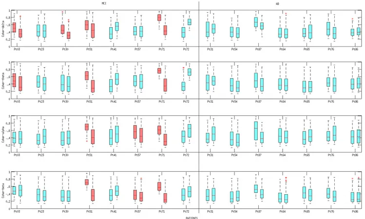
Four out of five stable MCI patients (pt 23, pt 41, pt 57, pt 72) showed stable or increased Coherence lev-els (i.e. stable or increased coupling strength), Figure 8, whereas pt 30 showed reduced Coherence levels, like the converted patients, and should be considered a false positive. On the contrary, from the PDI perspective, the totality of the stable MCI patients (pt 23, pt 30, pt 41, pt 57, pt 72) showed stable or reduced PDI (i.e. stable or increased coupling strength).
As regards Dm analysis, pt 23, pt 51 and pt 71 ex-hibited increased Dm levels (reduced coupling strength) in delta, alpha and beta band (Figure 9); pt 57 showed the same behaviour only in delta band and pt 72 only in theta band. Apparently, Dm seems to be not sensi-tive to MCI to AD conversion as there is no correlation between DM variation and disease progression towards AD. We can conclude that MCI patients who converted to AD exhibited:
• Decreased median Coherence in delta and theta bands (not specific because also one stable MCI patient, pt 30, exhibited a similar behaviour in delta band); • Increased median PDI and increased PDI range in
delta and theta bands (specific and sharp, particularly in delta band);
Summing all up, even though the analysed dataset is small, both Coherence and PDI resulted sensitive to the conversion from MCI to AD because both detected a reduced coupling strength in delta and theta bands. Nev-ertheless, Coherence looks less specific than PDI
be-February 15, 2017 10:20 WSPC/INSTRUCTION FILE paper˙PDI˙MCI˙AD˙IJNS˙v3
12 N. Mammone, L. Bonanno, S. De Salvo, S. Marino, P. Bramanti, A. Bramanti, Francesco C. Morabito
Fig. 7. Boxplot of PDI at time T0 and T1. Every row is associated to a specific EEG sub-band (delta, theta, alpha, beta). For each patient, the boxplot on the left represents the values assumed at time T0 whereas the boxplot on the right represents the values assumed at time T1. On each box, the central mark is the median, the edges of the box are the 25th and 75th percentiles, the whiskers extend to the most extreme data points not considered outliers. The red boxplots, in the MCI group, are associated to a statistically significant increase (p < 0.001) of PDI levels (see Section 6.3 Statistical Analysis.)
cause one stable MCI patient (patient 30) behaved like converted patients (patient 3, 51 and 71) as he/she ex-hibited a decreased coherence (Figure 8) in delta band, although at T1 he/she was still diagnosed MCI. From the PDI perspective, the reduced coupling strength in delta and theta bands was a behaviour that could be detected only on converted MCI patients.
6.3. Statistical analysis
In order to assess how significant was, for every patient, the overall variation of the PDI levels, between time T0 and T1, an intra-subject, descriptive analysis was per-formed. For every patient, given a sub-band, the two populations under analysis were the PDI values at T0 (given a patient, the boxplot on the left in Figure 7) and the PDI values at T1 (given a patient, the boxplot on the right in Figure 7). The same analysis was carried out with Coherence (Figure 8) and with Dm (Figure 9).
The Wilcoxon rank sum test40was used to test the null hypothesis that data in the two populations under consideration are independent samples from identical continuous distributions with equal medians. The
statis-tical analyses were performed in Matlab.
The achieved results are reported in Table II. The pvalues corresponding to a significant (p < 0.001) in-crease of PDI or Dm levels (reduced coupling strength) or with significant decrease of Coherence levels (re-duced coupling strength), are highlighted in bold style. In Figures 7, 8 and 9, the boxplots associated with sig-nificant (p < 0.001) increase of PDI or Dm levels or with significant decrease of Coherence levels, were coloured in red in MCI patients, in order to unravel pos-sible correlations with MCI progression towards AD.
As regards PDI analysis, the intrasubject variability study showed significantly (p < 0.001) increased PDI levels in: Patient 3 (delta, theta); Patient 51 (delta, theta, alpha, beta); Patient 57 (alpha, beta); Patient 71 (delta, theta, alpha, beta); Patient 54 (theta, alpha); Patient 87 (delta, theta, alpha, beta); Patient 64 (alpha); Patient 76 (theta, alpha, beta).
As regards Coherence analysis, the intrasubject variability study showed a significant (p < 0.001) de-crease of Coherence, between T0 and T1, in: Patient 3 (delta, theta); Patient 30 (delta); Patient 51 (delta, theta,
Fig. 8. Boxplot of Coherence at time T0 and T1. Every row is associated to a specific EEG sub-band (delta, theta, alpha, beta). For each patient, the boxplot on the left represents the values assumed at time T0 whereas the boxplot on the right represents the values assumed at time T1. On each box, the central mark is the median, the edges of the box are the 25th and 75th percentiles, the whiskers extend to the most extreme data points not considered outliers. The red boxplots, in the MCI group, are associated to a statistically significant decrease (p < 0.001) of Coherence levels (see Section 6.3 Statistical Analysis.)
alpha, beta); Patient 57 (alpha, beta); Patient 71 (delta, theta, alpha, beta); Patient 54 (theta, alpha); Patient 87 (delta, theta, alpha, beta); Patient 65 (beta); Patient 76 (delta, theta, beta).
As regards Dm analysis, the intrasubject variabil-ity study showed significantly (p < 0.001) increased Dm levels in: Patient 23 (delta, alpha and beta); Patient 51 (delta, alpha and beta); Patient 71 (delta, alpha and beta); Patient 57 (delta) and Patient 72 (theta).
Focusing on MCI patients, the intrasubject variabil-ity study showed that patients 3, 51 and 71 (who had converted to AD by the time T1) exhibited a significant (p < 0.001) increase of PDI in delta and theta bands and that patients 51 and 71 exhibited the same behaviour also in alpha and beta bands. As regards Coherence, pa-tients 3, 51 and 71 exhibited a significant (p < 0.001) decrease of Coherence in delta and theta bands and pa-tients 51 and 71 behaved similarly also in alpha and beta bands. However, also patient 30 (not converted to AD) exhibited a significant decrease of Coherence in delta band. As regards Dm analysis, it was not possible to de-tect a behaviour peculiar to the converted MCI.
Summing all up, a statistically significant increase of PDI medians was detected, in delta and theta bands, only in the MCI subjects who converted to AD. The av-erage increase of PDI, in delta and theta bands, might be possibly correlated with the reduced connectivity, which is associated to the disease progression towards AD. The group analysis was not performed, due to the limited size of the dataset: this will be the goal of our fu-ture research. A large number of patients is, indeed, cur-rently under recruitment at the IRCCS Neurolesi Center Bonino-Pulejo (Messina, Italy). In the near future, an extensive validation of the proposed methodology will be carried out on the extended dataset.
7. Discussion
In this paper, we introduced a novel measure of time series coupling, the Permutation Disalignment Index (PDI), and its possible application as an indirect estima-tion of the brain connectivity through the EEG, with ap-plication to the follow-up of AD and MCI patients. PDI is a multivariate measure which allows to estimate the
February 15, 2017 10:20 WSPC/INSTRUCTION FILE paper˙PDI˙MCI˙AD˙IJNS˙v3
14 N. Mammone, L. Bonanno, S. De Salvo, S. Marino, P. Bramanti, A. Bramanti, Francesco C. Morabito
Fig. 9. Boxplot of Dm at time T0 and T1. Every row is associated to a specific EEG sub-band (delta, theta, alpha, beta). For each patient, the boxplot on the left represents the values assumed at time T0 whereas the boxplot on the right represents the values assumed at time T1. On each box, the central mark is the median, the edges of the box are the 25th and 75th percentiles, the whiskers extend to the most extreme data points not considered outliers. The red boxplots, in the MCI group, are associated to a statistically significant increase (p < 0.001) of Dm levels (see Section 6.3 Statistical Analysis.)
coupling strength between signals in terms of projected alignment randomness. PDI overcomes the limitations of the standard univariate Permutation Entropy (PE)31 whenever a pairwise or multivariate measure is neces-sary. Furthermore, it overcomes the issues that come with applying standard, amplitude dependent method-ologies to EEG data. In fact, when processing the EEG,
the amplitude of the signals depends on the location of the reference electrode and, when using amplitude dependent methods, a preprocessing step to normalise EEG time series is required. The permutation concept allows us to bypass the normalisation as time series are projected into a symbolic space, where the effect of am-plitude is lost and only the effect of variation is kept,
which also produces an improved robustness to noise and EEG artifacts in general. The ability of PDI in de-tecting nonlinear interdependency of two unidirection-ally coupled Henon maps X and Y was validated theo-retically. PDI was then tested in a follow-up study over 8 MCI and 7 AD patients. Every patient was evaluated at time T0 and then three months later (time T1): 5 MCI remained stable and 3 MCI exhibited a conversion to AD. The EEG recordings were processed, in each sub-band, in order to track the changes of the EEG’s PDI in every range of frequency.
The study consisted in evaluating the evolution of PDI, all over the scalp, in comparison with Coherence and Dissimilarity Index. Coherence and PDI resulted both sensitive to the conversion from MCI to AD; in fact, MCI patients who converted to AD showed an in-creased median PDI and dein-creased median Coherence (reduced coupling strength) in delta and theta bands. However, only PDI resulted specific, because Coherence produced a false positive (a stable MCI subject exhibited a behaviour similar to the converted MCI). Analysing the EEG of MCI patients through PDI looks a promis-ing way to quantify how the disease is affectpromis-ing the EEG and to detect its possible degeneration towards AD. De-veloping EEG-based systems that are able to objectively quantify the progression of the disease is crucial and fo-cusing the attention on periodic, long-term, follow-up studies is necessary. In this way, we could unravel if the variation of key EEG features may be the hallmark of the disease’s progression and help to foresee its de-velopment. Furthermore, in the present paper, only rest-ing state EEG were considered, future work will also be focused on the analysis of EEG during tasks, includ-ing evoked potentials. In this case, however, the traces will be more likely to be affected by artifacts and an ad-vanced artifact rejection step will be required41,42,43,
44.
8. Conclusion
Permutation Disalignment Index (PDI) was proposed in this paper as a new measure of time series coupling, with application to the indirect estimation of the brain connectivity in patients affected by AD and MCI. PDI was tested on simulated two unidirectionally coupled Henon maps time series in order to test its ability to measure the coupling between interacting dynamic sys-tems. The simulation also yielded suggestions on how to tune the PDI parameters. PDI was then applied to real EEG traces recorded during a follow-up study car-ried out over 7 Alzheimer’s Disease (AD) patients and 8 Mild Cognitive Impairment (MCI) subjects. Every
pa-tient was evaluated at time T0 and at time T1, 3 months later. At time T1, 5 out of 8 MCI patients were still di-agnosed MCI, whereas the remaining 3 exhibited a con-version from MCI to AD. PDI was compared with the spectral coherence, a common parameter used in liter-ature in the analysis of AD and MCI EEG and with the Dissimilarity Index, a recent symbolic measure of time series dissimilarity. The study consisted in evaluat-ing the overall evolution of PDI, sub-band by sub-band. Both coherence and PDI resulted sensitive to the conver-sion from MCI to AD, but only PDI resulted specific as it allowed to detect a recurrent behaviour that was pecu-liar only to converted MCI patients, who indeed showed a significant increase of PDI in delta and theta bands (p<0.001). In conclusion, the intra-subject, longitudi-nal evaluation of the overall coupling between the EEG signals, through PDI, looks a promising method to dis-criminate between converted MCI and stable MCI. Fu-ture efforts will be focused on extending the study to a larger number of patients that should be monitored pe-riodically and over a long time. Furthermore, PDI will be tested, in conjunction with other EEG features, as a possible input parameter to a system designed for the estimation of the probability that a patient will convert to AD.
Acknowledgment
This work was funded by the Italian Ministry of Health, project code: GR-2011-02351397.
References
1. M. Prince, A. Comas-Herrera, M. Knapp, M. Guerchet, and M. Karagiannidou. World Alzheimer Report 2016. Alzheimer’s Disease International (ADI), London, 2016. 2. S. S. Poil, W. de Haan, W. M. van der Flier, H.D. Mansvelder, P. Scheltens, and K. Linkenkaer-Hansen. Integrative EEG biomarkers predict progression to Alzheimer’s disease at the MCI stage. Front Aging Neu-rosci., 58:12pp, 2013.
3. I. H. Ramakers, P. J. Visser, P. Aalten, A. Kester, J. Jolles, and F. R. Verhey. Affective symptoms as predictors of Alzheimer’s disease in subjects with Mild Cognitive Impairment: a 10-year follow-up study. Psychol Med., 40(7):1193–1201, 2010.
4. F. C. Morabito, M. Campolo, D. Labate, G. Morabito, L. Bonanno, A. Bramanti, S. de Salvo, A. Marra, and P. Bramanti. A longitudinal EEG study of Alzheimer’s disease progression based on a complex network ap-proach. Int J Neural Syst, 25(2):1550005(1–18), 2015.
5. H. Adeli, S. Ghosh-Dastidar, and
compu-February 15, 2017 10:20
WSPC/INSTRUCTION FILE
paper˙PDI˙MCI˙AD˙IJNS˙v3
16 N. Mammone, L. Bonanno, S. De Salvo, S. Marino, P. Bramanti, A. Bramanti, Francesco C. Morabito
tation: Imaging, classification, and neural models.
Jour-nal of Alzheimer’s Disease, 7(3):187–199, 2005.
6. H. Adeli, S.
Ghosh-Dastidar, and N. Dadmehr. Alzheimer’s disease: Models of computation and analysis of EEGs. Clinical EEG and Neuroscience, 36(3):131–140, 2005.
7. J. Jeong. EEG dynamics in patients with Alzheimer’s disease. Clin Neurophysiol., 115(7):1490–1505, 2004. 8. F. Hatz, M. Hardmeier, N. Benz, M. Ehrensperger,
U. Gschwandtner, S. Regg, Schindler C., Monsch U., and Fuhr P. Microstate connectivity alterations in pa-tients with early Alzheimer’s disease. Alzheimer’s Re-search and Therapy, 7(78), 2015.
9. N. Mammone, F. C. Morabito, and J. C. Principe. Visu-alization of the short term maximum lyapunov exponent topography in the epileptic brain. In Proc. of 28th Annual Intern. Conf. IEEE Eng. Med. Biol. Soc. (EMBC), pages 4257–4260, New York City, USA, 2006.
10. N. Mammone, J.C. Principe, F.C. Morabito, D.S. Shiau, and J. C. Sackellares. Visualization and modelling of STLmax topographic brain activity maps. Journal of neuroscience methods, 189(2):281–294, 2010.
11. E. Ferlazzo, N. Mammone, V. Cianci, S. Gasparini, A. Gambardella, A. Labate, M.A. Latella, V. Sofia, M. Elia, F.C. Morabito, and U. Aguglia. Permutation en-tropy of scalp EEG: A tool to investigate epilepsies: Sug-gestions from absence epilepsies. Clinical Neurophysiol-ogy, 125(1):13–20, 2014.
12. N. Mammone and F.C. Morabito. Analysis of absence seizure EEG via permutation entropy spatio-temporal clustering. Proc. of Intl. Joint Conf. on Neural Networks, (IJCNN):1417–1422, 2011.
13. C. J. Stam, Y. van der Made, Y. A. Pijnenburg, and P. Scheltens. EEG synchronization in Mild Cognitive Impairment and Alzheimer’s disease. Acta Neurol Scand, 108(2):90–96, 2003.
14. J. J. Dunkin, A. F. Leuchter, T. F. Newton, and I. A. Cook. Reduced EEG coherence in dementia: state or trait marker? Biol Psychiatry, 35:870–879, 1994. 15. Z. Sankari, H. Adeli, and A. Adeli.
Intrahemi-spheric, interhemiIntrahemi-spheric, and distal EEG coherence in Alzheimer’s disease. Clin Neurophysiol., 122(5):897– 906, 2010.
16. Z. Sankari and H. Adeli. Probabilistic neural networks for diagnosis of Alzheimer’s disease using conven-tional and Wavelet coherence. J Neurosci Methods, 197(1):165–170, 2011.
17. Z. Sankari, H. Adeli, and A. Adeli. Wavelet coherence model for diagnosis of Alzheimer disease. Clin EEG Neurosci., 43(4):268–278, 2012.
18. D. V. Moretti. Conversion of Mild Cognitive Impairment patients in Alzheimer’s disease: prognostic value of al-pha3/alpha2 electroencephalographic rhythms power ra-tio. Alzheimers Res Ther., 7(80):14pp, 2015.
19. D. V. Moretti, A Prestia, C. Fracassi, C. Geroldi, G. Bi-netti, P. M. Rossini, O. ZaBi-netti, and G. B. Frisoni.
Volu-metric differences in mapped hippocampal regions cor-relate with increase of high alpha rhythm in Alzheimer’s disease. Int J Alzheimers Dis., Article ID 208218:7pp, 2011.
20. D. V. Moretti, G. B. Frisoni, G. Binetti, and O. Zanetti. Anatomical substrate and scalp EEG markers are correlated in subjects with Cognitive Impairment and Alzheimer’s disease. Front Psychiatry, 1(Article 152):9pp, 2011.
21. P. Giannakopoulos, P. Missonnier, E. Kvari, G. Gold, and A. Michon. Electrophysiological markers of rapid cogni-tive decline in Mild Cognicogni-tive Impairment. Front Neurol Neurosci., 24:39–46, 2009.
22. L. S. Prichep. Quantitative EEG and electromagnetic brain imaging in aging and in the evolution of demen-tia. Ann N Y Acad Sci., 1097:156–167, 2007.
23. P. M. Rossini, C. Del Percio, P. Pasqualetti, E. Cas-setta, G. Binetti, G. Dal Forno, F. Ferreri, G. Frisoni, P. Chiovenda, C. Miniussi, L. Parisi, M. Tombini, F. Vec-chio, and C. Babiloni. Conversion from Mild Cognitive Impairment to Alzheimer’s disease is predicted by sources and coherence of brain electroencephalography rhythms. Neuroscience, 143(3):793–803, 2006.
24. R. A. Sperling, P. S. Aisen, L. A. Beckett, D. A. Bennett, S. Craft, A. M. Fagan, T. Iwatsubo, C. R. Jr Jack, J. Kaye, T. J. Montine, D. C. Park, E. M. Reiman, C. C. Rowe, E. Siemers, Y. Stern, K. Yaffe, M. C. Carrillo, B. Thies, M. Morrison-Bogorad, M. V. Wagster, and C. H. Phelps. Toward defining the preclinical stages of Alzheimer’s disease: recommendations from the national institute on aging-Alzheimer’s association workgroups on diagnos-tic guidelines for Alzheimer’s disease. Alzheimers De-ment., 7(3):280–292, 2011.
25. A. Alberdi, A. Aztiria, and A. Basarab. On the early di-agnosis of Alzheimer’s disease from multimodal signals: A survey. Artif Intell Med., 71:1–29, 2016.
26. M. Buscema, E. Grossi, M. Capriotti, C. Babiloni, and P. Rossini. The IFAST model allows the prediction of conversion to Alzheimer disease in patients with mild cognitive impairment with high degree of accuracy. Curr Alzheimer Res, 7(2):173–187, 2010.
27. M. Buscema, F. Vernieri, G. Massini, F. Scrascia, M. Breda, PM. Rossini, and et al. An improved I-FAST system for the diagnosis of Alzheimer’s disease from un-processed electroencephalograms by using robust invari-ant features. Artif Intell Med, 64(1):59–74, 2015. 28. G. Ouyang, C. Dang, D. A. Richards, and X. Li.
Ordi-nal pattern based similarity aOrdi-nalysis for EEG recordings. Clin Neurophysiol., 121(5):694–703, 2010.
29. American Psychiatric Association, editor. Diagnostic and statistical manual of mental disorders (5th ed.). 2013.
30. A. Delorme and S. Makeig. EEGLAB: An open source toolbox for analysis of single-trial EEG dynamics
in-cluding Independent Component Analysis. Journal of
31. C. Bandt and B. Pompe. Permutation entropy: A natural complexity measure for time series. Phys. Rev. Lett., 88 (17), 2002.
32. X. Zhao, P. Shang, and J. Huang. Permutation complex-ity and dependence measures of time series. EPL (Euro-physics Letters), 102(4):40005, 2013.
33. N. Mammone, J. D. Henriksen, T. W. Kjaer, and F. C. Morabito. Differentiating interictal and ictal states in childhood absence epilepsy through Permutation Renyi Entropy. Entropy, 17(7):4627–4643, 2015.
34. A. Renyi. On measures of information and entropy. Proc. of the fourth Berkeley Symposium on Mathemat-ics, Statistics and Probability, pages 547–561, 1961. 35. R. Quian Quiroga, J. Arnhold, and P. Grassberger.
Learn-ing driver-response relationships from synchronization patterns. Physical Review E, 61(5):5142–5148, 2000. 36. C. J. Stam and B. W. van Dijk. Synchronization
likeli-hood: an unbiased measure of generalized sysnchroniza-tion in multivariate data sets. Physica D, 163:236–251, 2002.
37. S. Boccaletti, J. Kurths, G. Osipov, D. L. Valladares, and C. S. Zhou. The synchronization of chaotic systems. El-sevier, 2000.
38. F.C. Morabito, D. Labate, F. La Foresta, A. Bra-manti, G. Morabito, and I. Palamara. Multivariate multi-scale permutation entropy for complexity analysis of Alzheimer’s disease EEG. Entropy, 14(7):1186–1202,
2012.
39. P. D. Welch. The use of Fast Fourier Transform for the estimation of power spectra: A method based on time averaging over short, modified periodograms. IEEE Transactions on Audio and Electroacoustics, 15(2):70– 73, 1967.
40. H. B. Mann and Whitney D. R. On a test of whether one of two random variables is stochastically larger than the other. Ann. Math. Statist., 18(1):50–60, 1947.
41. N. Mammone and F. C. Morabito. Independent
ComponentAnalysis and high-order statistics for
auto-matic artifact rejection. In 2005 International Joint Con-ference on Neural Networks, pages 2447–2452, Montral, Canada, 2005.
42. N. Mammone, G. Inuso, F. La Foresta, and F. C. Mora-bito. Multiresolution ICA for artifact identification from electroencephalographic recordings. Lecture Notes in Artificial Intelligence, 4692:680–687, 2007.
43. N. Mammone, F. La Foresta, and F. C. Morabito. Auto-matic artifact rejection from multichannel scalp EEG by Wavelet ICA. In Sensors Journal IEEE, 12(3):533-42, 2012.
44. N. Mammone and F. C. Morabito. Enhanced Automatic
Wavelet Independent Component Analysis
for Electroencephalographic Artifact Removal. Entropy, 16(12):6553–6572, 2014.