UNIVERSITA' DEGLI STUDI DEL MOLISE
DIPARTIMENTO DI BIOSCIENZE E TERRITORIO
______________________________________________________________________________________ DOTTORATO DI RICERCA IN: SCIENZE FORESTALI, DELLE TECNOLOGIE
AGRO-INDUSTRIALI E DEL TERRITORIO RURALE. I SISTEMI FORESTALI
Ciclo XXVII
C
OMPARING
S
INGLE
T
REE AND
A
REA
B
ASED
A
PPROACHES
FOR
B
IOMASS
E
STIMATION OF
C
APE
V
ERDEAN
X
EROPHYTIC
F
ORESTS
U
SING
V
ISIBLE
A
ERIAL
I
MAGERY
SETTORE SCIENTIFICO-DISCIPLINARE AREA 07AGR/05
COORDINATORE: Chiar.mo Prof. MARCO MARCHETTI TUTORE: Chiar.mo Prof. GHERARDO CHIRICI
DOTTORANDO: LUCA BERNASCONI
i COORDINATORE:
Chiar.mo Prof. MARCO MARCHETTI
TUTORE:
Chiar.mo Prof. GHERARDO CHIRICI
ii
A
BSTRACTITALIAN:
Con base in ortofoto aeree ad alta risoluzione sono stati sviluppati modelli per la stima della biomassa di foreste xerofile capoverdiane.
Il metodo proposto si basa sull'integrazione di tecniche di clustering in combinazione con l'indice VARI (Visibile Atmospherically Resistant Index) e algoritmi di segmentazione per l'estrazione chiome degli alberi. Questo procedimento ha permesso la minimizzazione dei problemi dovuti alla scarso contrasto spettrale tra il suolo e le chiome nelle parti più luminose e quelle in ombra.
Sono stati testati metodi basati sul singolo albero e per area (area based) e le loro prestazioni sono state contrastate con i dati dell´inventario forestale nazionale di Capo Verde (CV-IFN). Nel primo approccio la biomassa è stata calcolata in funzione della larghezza della chioma e l'altezza degli alberi, utilizzando le equazioni allometriche sviluppate appositamente per l´inventario CV-IFN. Nel secondo approccio si è usata l'analisi di regressione per derivare modelli per la stima della biomassa in funzione dell'area proiettata della chioma.
L´accuratezza delle stime è stata misurata analizzando l´ RMSE (Root Mean Square Error) tra la biomassa stimata e quella osservata.
L´errore osservato nei due modelli è simile, variando tre il 42% del primo approccio e il 45% del secondo.
iii La biomassa media calcolata per l´intera area di studio (14.399 ettari) con base nei dati del CV-IFN, è di 12,701 Mg ha-1. Questo a fronte di 11,380 Mg ha-1 stimato dal modello per area (area based) e 10,278 Mg ha-1 per il modello per singolo albero.
Una stratificazione dell´immagine per aree omogenee, definite da mappe del soprassuolo più precise, può portare a stime di biomassa piú accurate. I modelli proposti aprono spazi per l´applicazione pratica sia a fini di monitoraggio che di gestione delle risorse forestali.
ENGLISH:
Models to estimate the AGB over dry Cape Verdean woodlands were developed using visible high-resolution aerial orthophotography.
The proposed method is based on the integration of clustering techniques combined with the Visible Atmospherically Resistant Index (VARI) and segmentation algorithms for tree crowns extraction. This allowed for the minimization of constraints due to poor spectral contrast between the background and tree crowns, especially for brighter parts of the crowns and shadowed parts of the scene.
Both single tree and area based approaches were tested and their performances compared on the basis of field data from the National Forest Inventory of Cape Verde (CV-NFI). In the first approach, AGB was calculated as a function of crown width and tree height by the allometric equations developed specifically within the CV-NFI. In the second approach, regression analysis was used in deriving models for biomass as a function of the crown projected area.
iv The accuracy of the values predicted was measured by the Root Mean Square Error (RMSE) against the allometric-based (field-measured) biomass.
The models produced similar accuracy in the AGB predictions with NRMSE% of 42% for the first approach and 45% for the second.
The mean AGB as estimated from the CV-IFN data for the study area of 14399 ha was 12.701 Mg ha-1. This compared with 11.380 Mg ha-1 predicted by the area based model and 10.278 Mg ha-1 by the single tree model.
The findings demonstrate that promising results can be achieved and as expected, the reliability increases with the area for which mean values are presented. Improvements of the forest maps and the stratification in homogeneous layers can lead to enhanced AGB estimations, something which opens opportunities for the practical application of the models for monitoring and management purposes.
KEYWORDS
Aboveground biomass, high spatial resolution visible aerial imagery, remote sensing, xerophytic forests, Prosopis sp., Cape Verde.
v ACKNOWLEDGEMENTS
I would like to start expressing my gratitude to those who contributed in the construction of the bases that today are allowing the presentation of this work. I would be remiss if I did not mention Sabrina Raddi who supported my first steps in world of research by encouraging me and transmitting her knowledge.
My deepest gratitude to my coordinator, Prof. Marco Marchetti, for his constant encouragement, support, and guidance during this challenging process due to the distance and time limitations and to my adviser and Prof. Gherardo Chirici, who expertly guided this work during all phases, with the greatest support and availability .
I am grateful to the staff of the Forestry Department of the Ministry of Rural Development of Cape Verde who shared with me the vast experience of National Forestry Inventory. That experience is at the center of the reflections that permitted the conception and execution of this research.
Thanks to the IFER and especially to Petr Blazek and Martin Cerny who were always available to discuss the methods for the collection and treatment of the data that are the foundation of this research.
My recognition to my colleagues at the University of Molise—Marco Ottaviano, Daniela Tonti, Matteo Mura—who supported me greatly during the firsts phases of image processing and contributed with their generosity to reduce the distances between Cape Verde and Isernia.
My sincere thanks go to my wife Maria del Mar and to my daughters Giulia e Sofia, my family, friends and colleagues for their support and patience during these tireless months of dedication which have often kept me away from them.
vi TABLE OF CONTENTS
ABSTRACT ... i
TABLE OF CONTENTS: ...vi
1. INTRODUCTION ... 1
2. MATERIALS ... 15
2.1 STUDY AREA ... 15
2.1.1 STUDY AREA CHARACTERIZATION ... 19
2.2 FIELD DATA ... 23
2.3 AERIAL PHOTOS ... 25
3. METHODS ... 26
3.1 AGB ESTIMATION USING IMAGERY DATA ... 26
3.1.1 TREE CROWN MAPPING ... 26
3.1.2 TREE CROWN EXTRACTION AND CPA CALCULATION... 32
3.1.3 TREE HEIGHT MODELLING ... 36
3.1.4 BIOMASS CALCULATION ... 37
3.2 ACCURACY ASSESSMENT ... 38
4. RESULTS ... 40
4.1 TREE CROWNS MAPPING ... 40
4.2 MODELS TUNING ... 41
4.3 TREE CROWN PROJECTED AREA CALCULATION ... 41
4.4 TREE DENSITY ... 43
4.5 BIOMASS CALCULATION ... 43
5. DISCUSSION AND CONCLUSIONS ... 48
5.1 SOURCES OF ERROR ... 54
5.2 LIMITATIONS AND RECOMMENDATIONS FOR FUTURE INVESTIGATION ... 57
6. REFERENCES ... 59
vii FIGURES
Figure 1: Localization of Cape Verde ... 15
Figure 2: Localization of the study area in Santiago Island ... 20
Figure 3: Aspects of the woodlands that are object of this study ... 21
Figure 4: Detail of forest map and field plots in the study area. ... 23
Figure 5: Histogram indicating the frequency of pixels that belong to each seed cluster ... 27
Figure 6: Result of ISOCLUST classification ... 28
Figure 7: Tree canopy map obtained by VARI image processing ... 28
Figure 8: The VARI of a portion of the scene. ... 31
Figure 9: Overlap between the RGB and the ISOCLUST+VARI reclassified image for classification accuracy assessment ... 31
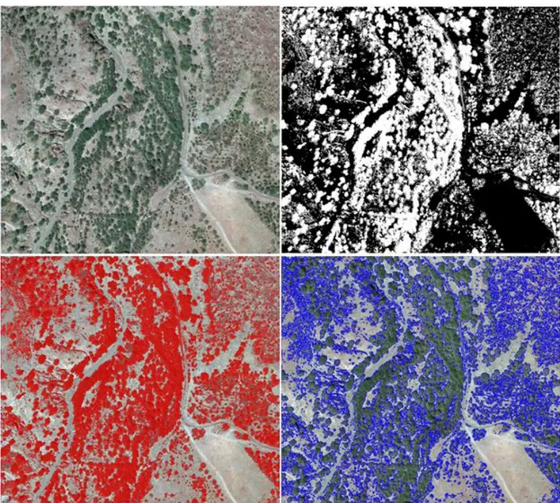
Figure 10: Sequential steps of image processing from the composite RGB image (a) to the ISOCLUST +VARI fusion (b) and threshold classification (c) and segmentation (d). ... 32
Figure 11: Comparison between field measured crowns (red polygons) and segments obtained by image processing (green polygons). ... 34
Figure 12: Comparison between different setting of color/shape and smoothness/compactness. The blue lines represent the results of higher compactness (1) and the red lines higher smoothness (0), the black lines represent the field plot and crowns. A) color/shape 0.5 smoothness/compactness 1; B) color/shape 0.5 smoothness/compactness 0; C) color/shape 1 smoothness/compactness 1; D color/shape 0 smooth-ness/compactness 0. ... 35
viii Figure 13: Relation between horizontal crown area and tree height for Prosopis sp. in Santiago island ... 36 Figure 14: Relation between tree crown area and biomass... 38 Figure 15: The final result of tree crowns mapping in a portion of the scene. ... 40 Figure 16: Relation between observed and predicted CPA, m2 per plot (500m2), in the single tree approach. The CPA is the sum of the individual’s segments area having their centroid inside the plots ... 42 Figure 17: Relation between observed and predicted CPA, m2 per plot (500m2), in the area based approach. Figure A is the extracted CPA from the circular plots at original resolution. Figure B represents the CPA extracted from the spatialized map at 500m2 pixel resolution. ... 42 Figure 18: Relation between predicted and observed tree density nr ha-1 ... 43 Figure 19: The edge effect in the area based approach (model) when the field plot with the emerging crowns shapes (green area) are used as feature definition image ... 44 Figure 20: Relation between observed and predicted AGB, Kg per plot (500m2), in the area based approach. The figure A is the estimated AGB from the circular plots at original resolution. Figure B represents the AGB extracted from the spatialized map at 500m2 pixel resolution. ... 45 Figure 21: Relation between observed and predicted AGB, Kg per plot (500m2), in the single tree approach. The figure A is the AGB calculated as sum of the
individual’s segments AGB having their centroid inside the plots. Figure B represents the AGB extracted from the spatialized map at 500m2 pixel resolution. ... 45
ix Figure 22 Relation between observed and predicted AGB, Kg per plot (500m2) when the reference AGB is calculated using only the crowns portions falling inside the plots. In the figure A is contrasted with the AGB predicted by area based approach and in figure B with the single tree approach. ... 46 Figure 23: Distribution of the biomass observed and predicted by the two models.49 Figure 24: Distribution of the biomass in the single approach ... 50 Figure 25: Distribution of the biomass in the area based approach ... 50 Figure 26: Trend of the relative standard error at increasing number of sampling plots for the observed AGB variability in the study area. The point represents the RSE at the given number of samples in the study area. ... 57 Figure 27: AGB map of the study area expressed in Mg Ha-1 ... 82
x TABLES
Table 1: A summary of major characteristics of biomass calculation from field
measurements (adapted from Lu et al. 2014) ... 2 Table 2: Potential variables used in a biomass estimation procedure (adapted from Lu et al. 2014) ... 4 Table 3: Afforestation of cape Verdean islands (source Direcção dos Serviços
Florestais) ... 19
Table 4: Mean, standard deviation and coefficient of variation of main
dendrometrics parameters describing the forest type in the study area ... 22 Table 5: The characteristic of the imagery used in the study... 25 Table 6: Description of the clusters resulting from the ISOCLUST classification and new values assigned by reclassification algorithm ... 29 Table 7: Variation of the R2 and RMSE% at different thresholds ... 33 Table 8: Comparison between predicted versus observed AGB in the study area (14399 ha) ... 53 Table 9: Average AGB, confidence interval and relative standard error (RSE %) for the study area. ... 57
xi ACRONYMS
AD Absolute deviation
AGB Above ground biomass
ANN Artificial neural network APE Absolute percentage error ASL Airborne Laser Scanner
CHM Canopy Height Model
CIR Color-infrared
CPA Crown projected area
CV-NFI Cape Verdean National Forest Inventory DBH Diameter at breast height
FMDC Field-Map Data Collector FMIA Field-Map Inventory Analyst GLCM Gray level co-occurrence matrix GSSN Global navigation satellite system
IFER Institute of Forest Ecosystem Research, Ltd InSAR Interferometry SAR
KNN k-nearest neighbor
LIDAR Light Detection and Ranging NFI National Forestry Inventory
NIR Near Infrared
NRMSE Normalized root mean square error PCA Principal Component Analysis
xii Pol-InSAR Polarimetric SAR Interferometry
RGB Red Green Blue
RMSE Root Mean Square Error RSE Relative Standard Error SAR Synthetic Aperture Radar SMA Spectral Mixture Analysis SVM Support Vector Machines SAR Synthetic Aperture Radar
SE Standard Error
TCT Tasseled Cap Transform
1
1. I
NTRODUCTIONTree biomass is useful in assessing forest structure and condition to estimate forest productivity and carbon fluxes; in providing a means of assessing sequestration of carbon in wood, leaves, and roots; and also as an indicator of both the biological and economic value of a forest ecosystem. Thus, the estimation of forest biomass at different geographical scales (from local to global) becomes significant in reducing uncertainty of carbon emission and sequestration, measures of land degradation or restoration, and understanding the roles that forests play in environmental processes and sustainability (Foody 2003).
In arid and sub-arid areas, rural populations depend greatly on the sparse scrublands and woodlands for fuelwood and pasture for animals. In such contexts, quick and cost-effective estimation of biomass availability and variation is crucial to implementing proper management practice. This is the case of Cape Verde where, since independence, nationwide campaigns and relevant efforts were realized to promote afforestation of vast arid areas. These woodlands, composed by shrub-like xerophytic trees, although expressing a limited economic value, support significant socio-economic and ecological functions. In this context, the accessibility of simple, fast and inexpensive methods for biomass and forest cover estimation are essential to promoting the monitoring and management of these resources.
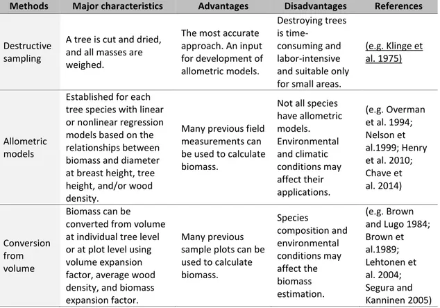
The most accurate method by which to estimate forest biomass is based on field measurements, but collection of field measurements is time-consuming and labor-intensive. Moreover, it is impossible to census large geographic areas (Segura and Kanninen 2005; Seidel et al. 2011; Wang et al. 2011), thus it is only suitable for a
2 small area and cannot provide spatial distribution. Thus, direct collection is generally used to obtain biomass reference data and to develop species-specific allometric models based on measured attributes, such as diameter at breast height (DBH), tree height, crown projected area (CPA) and/or wood density (table 1). Then the allometric models can be used to estimate the AGB for a specific tree, as a function of these parameters for stand biomass inventories.
Table 1: A summary of major characteristics of biomass calculation from field measurements
(adapted from Lu et al. 2014)
Regional or national forest inventories have large tree-volume datasets at plot level and forests stand so the conversion of tree volume to biomass on the basis of the average wood density can greatly reduce time and cost (Lu et al. 2014). However, this approach is not appropriate in woodlands, composed of shrub-like xerophytic
Methods Major characteristics Advantages Disadvantages References
Destructive sampling
A tree is cut and dried, and all masses are weighed.
The most accurate approach. An input for development of allometric models. Destroying trees is time-consuming and labor-intensive and suitable only for small areas.
(e.g. Klinge et al. 1975)
Allometric models
Established for each tree species with linear or nonlinear regression models based on the relationships between biomass and diameter at breast height, tree height, and/or wood density.
Many previous field measurements can be used to calculate biomass.
Not all species have allometric models. Environmental and climatic conditions may affect their applications. (e.g. Overman et al. 1994; Nelson et al.1999; Henry et al. 2010; Chave et al. 2014) Conversion from volume Biomass can be converted from volume at individual tree level or at plot level using volume expansion factor, average wood density, and biomass expansion factor.
Many previous sample plots can be used to calculate biomass. Species composition and environmental conditions may affect the biomass estimation. (e.g. Brown and Lugo 1984; Brown et al.1989; Lehtonen et al. 2004; Segura and Kanninen 2005)
3 trees, where the ecological and economic interest is focused on the biomass and the measurement of the volume is a challenging task.
A wide range of techniques has been used for biomass estimation. For example, Wang et al. (2009) divided estimation approaches into (1) process model-based; (2) empirical model-based; (3) biomass expansion/conversion factor or coefficient-based; and (4) integration of plot and remotely sensed data (Lu et al. 2014).
Process-based ecosystem models employ biogeochemical processes, including photosynthesis, absorption, and carbon allocation. The models generally include biology, soil, climate, hydrology, and anthropogenic effects (Smyth et al. 2013). Constraints in data source (e.g. climate data, soil, and topography), spatial resolution, and inaccuracy of models often result in high uncertainties in biomass estimates (Rivington et al. 2006; Zhang et al. 2012). Process-based ecosystem models assume homogeneous stands and lack the ability to provide spatial variability in forest biomass. Conversely, remote sensing has the capability to consistently capture land surface features over large areas. (Lu et al. 2014).
In past decades, an increasing number of researches have explored the suitability and applied remote sensing-based models to provide accurate biomass estimation across different ecosystems and at different geographical scales.
Remotely sensed data collected by optical multispectral and hyperspectral sensor, radar and Lidar combined with techniques based on empirical regression models and nonparametric algorithms are commonly used to estimate above ground biomass (AGB) of forested landscapes (Goetz et al. 2009), (Gleason and Im 2011), (Katoh and Gougeon 2012), (Vaglio Laurin et al. 2014), (Huang, Y. P., and J. S. Chen.
4 2013), (Hudak, A. T., et al, 2012), (Muukkonen and Heiskanen 2007; Blackard et al. 2008; García et al. 2010; Mitchard et al. 2011) (table 2).
Category Variables Description References
Optical sensor data
Spectral features
Spectral bands, vegetation indices, and transformed images
(e.g. Foody et al. 2003; Zheng et al.2004)
Spatial features Textural images and segments from the spectral bands
(e.g. Lu and Batistella 2005) Subpixel
features
Fractional features such as green vegetation and NPV by unmixing the multispectral image
(e.g. Lu et al. 2005) Combination of
spectral and spatial features
Combination of images such as spectral bands, vegetation indices, and textural images as extra bands
(e.g. Lu 2005; Lu et al. 2012) Active sensor data Radar
Backscattering coefficients, textural images, interferometry SAR, and Polarimetric SAR interferometry can be used as variables (e.g. Mitchard et al. 2011; Nafiseh et al. 2011; Saatchi et al. 2011b; Carreiras et al. 2012; Sarker et al.2012) Lidar
Lidar metrics based on statistical measures of point clouds or estimated products (e.g. CHM or individual trees) can be used as variables
(e.g. Popescu et al. 2011; Nelson et al.2012; Chen 2013; Skowronski et al.2014) Combination of radar and lidar data
For mapping biomass over large areas where field plots are scarce, lidar samples (e.g. strips) can be taken. Lidar-derived biomass calibrated by field data is then used as dependent variable, and radar data are used as independent variables for developing biomass estimation models. Lidar-derived biomass serves as “virtual” field data to create a spatially representative biomass “truth” dataset for mapping biomass wall-to-wall using radar data.
(e.g. Sun et al. 2011; Tsui et al. 2013) Integration of optical and/or active sensor data Fusion of different sensor data e.g. optical and radar data
Fusion of Landsat and radar data to generate an enhanced multispectral image using different techniques such as wavelet-merging. (e.g. Chen 2013; Montesano et al.2013) Combination of optical and radar or lidar as extra variables
Lidar and/or radar data are combined with optical-sensor multispectral bands as extra variables (e.g. Nelson et al. 2009; Chen et al.2012; Selkowitz et al. 2012; Pflugmacher et al. 2014; Vaglio Laurin et al. 2014)
5 Optical sensor data are commonly used for biomass estimation; they can produce data at various spatial, spectral, radiometric, and temporal resolutions that are suitable in extracting variables for biomass estimation. Many techniques, such as vegetation indices, image transformation algorithms (e.g. principal component analysis, PCA; minimum noise fraction transform; and tasselled cap transform, TCT), texture measures, and spectral mixture analysis (SMA), have been used to produce new variables from optical multispectral data (Lu 2006).
The methods are based on spectral responses (spectral bands or vegetation indices and transformed images) (Bannari et al. 1995; McDonald et al. 1998 Foody et al. 2003; Zheng et al.2004), textural images (e.g. the gray level co-occurrence matrix (GLCM)-based texture measures) (Lu and Batistella 2005; Kuplich et al. 2005; Kayitakire et al. 2006; De Grandi et al. 2009; Sarker et al. 2012) or the combination of both (Lu 2005; Lu et al. 2012).
Several studies establish that methods based on spectral responses perform better when the forest stand structure is relatively simple (Lu et al. 2004; Lu 2005), while the textural images are more important in complex forest stand structures. The combination of the two methods improved biomass estimation compared to the use of individual spectral responses or textural images alone (Lu 2005).
Limitations in the application of optical sensors are related to saturation problems for forest sites with high biomass density and the influence of external factors such as atmosphere, soil moisture, vegetation phenology, and growth vigor spectral-based variables. They are suitable for the retrieval of horizontal vegetation structures such as vegetation types and canopy cover, but not for estimation of
6 critical parameters for biomass estimation such as tree and canopy height. Some optical sensor data such as ALOS/PRISM, Terra ASTER, and SPOT provide a stereo-viewing capability that can be used to develop vegetation canopy height, thus improving biomass estimation performance (St‐Onge et al. 2008; Ni et al. 2014).
Long wavelength radar data are an important data sources for biomass estimation, especially when optical sensor data are not available due to the cloud cover in tropical regions.
Synthetic aperture radar (SAR) is a promising approach for studying forest biomass because of its ability in penetrating forest canopy to a certain depth, its sensitivity to water content in vegetation, and weather independency (Le Toan et al. 1992, 2011; Dobson et al. 1995; Kasischke et al. 1997; Huang and Chen 2013). The regression technique based on backscattering amplitudes (Santos et al. 2002; Sandberg et al. 2011; Rahman and Sumantyo 2013) and the interferometry technique based on backscattering amplitudes and phases (Balzter et al. 2007) are commonly used in biomass estimation (Lu et al., 2014). Because of the high correlation between vegetation canopy height and biomass, InSAR capability in providing vegetation height feature provides a promising tool for large-scale biomass estimation. This is especially important for tropical and subtropical regions because of the cloud-cover issue (Kellndorfer et al. 2004; Solberg et al. 2014).
The Polarimetric SAR interferometry (Pol-InSAR), a combined polarization and interferometry, is a recently developed radar remote sensing technology. Pol-InSAR produces more sensitive characteristics in spatiality as well as in shape and direction than interferometry or polarimetry for forest diffusions (Lu, et al., 2014). A
7 common biomass estimation procedure is primarily to estimate forest height using coherence information (Cloude and Papathanassiou 2003) and then convert it to biomass through correlation analysis (Garestier and Le Toan 2010).
The major limitations are connected to the possibility of distinguishing vegetation types (Li et al. 2012) and to the noise and outliers in the data, thus resulting in difficulty in biomass estimation. Nevertheless, these techniques are attracting increasing interest considering the referred capacity in penetrating complex forests structures, the high correlation between vegetation canopy height and biomass and weather independency.
Data saturation in optical and radar data is an important factor influencing the accuracy of biomass estimation in forests with complex stand structures, on the contrary lidar is capable to extract canopy height information even at high levels (>1000 Mg ha-1; e.g. Means et al. 1999).
Because of the capability of lidar in providing both horizontal and vertical information of the canopy structures, its use leads to better biomass estimation performance than individual optical or radar data (Clark et al. 2011). In airborne lidar data, metrics can be extracted on the basis of either individual trees or areas (Chen 2013; Barbati et al, 2009; Corona and Fattorini 2008). The individual tree-based approach requires identifying tree features such as treetop (e.g. Popescu et al. 2002; Chen et al. 2006), crown radius (e.g. Popescu et al. 2003), or crown boundary (e.g. Chen et al. 2006; Zhen et al. 2014). Mapping individual trees requires high lidar data point density (generally 10 points per m2 or higher) and is
8 challenging in closed and multilayer canopies such as tropical rainforests (Lu e t al., 2014).
The area-based approach, which generates statistical metrics from laser returns or canopy height model (CHM) constructed from the returns, has been widely used (e.g. Lim et al. 2003; Chen et al. 2012; Lu et al. 2012; Chirici et al. 2016).
In the past, airborne lidar data were mainly applied in small areas due to high costs and large volume. As technologies advance, the use of airborne lidar data for biomass mapping will expand from local to regional levels (e.g. Skowronski and Lister 2012). For regional- to global-scale applications, spaceborne lidar – ICESat GLAS – was available between 2003 and 2009, and the use of GLAS data for biomass estimation has been shown to be valuable (Lefsky et al. 2005; Simard et al. 2008; Nelson 2010; Miller et al. 2011; Popescu et al. 2011; García et al. 2012).
The combination of airborne lidar and satellite imagery is another promising approach for large-area biomass mapping. Optical sensors, radar, and lidar each have pros and con and proper integration of them can improve biomass estimation accuracy (Walker et al. 2007; Kellndorfer et al. 2010).
Optical sensor data mainly represent land cover surface features, and radar data, especially with long wavelengths, can penetrate forest canopies to a certain depth capturing information about stems, branches, and understories. This providing more vertical stand structure information for vegetation types (Lu at al., 2014).
Lidar data are powerful for estimating canopy structure but has limited spectral information because laser point intensity is from one wavelength. Optical sensors
9 provide rich spectral information but the spectral reflectance does not have a strong relationship with canopy structure. Thus, lidar and optical sensor data are highly complementary. However, earlier studies that integrated lidar with optical data have reported mixed results. Some studies have shown that the addition of optical to lidar data registered only slight or no improvement in biomass estimation (e.g. Hyde et al. 2006; Clark et al. 2011; Latifi et al. 2012). Conversely, Anderson et al. (2008) and Vaglio Laurin et al. (2014) found that integration of lidar and hyperspectral data significantly improved biomass estimation.
The extent and complexity of a study area are the conditioning elements in the selection of suitable remote sensing data and biomass estimation algorithms. Thus, the integration of the proprieties of the different remote sensing data sources allows sufficient flexibility to cover different scales and conditions. Multiscale data from high spatial resolution datasets, such as QuickBird and lidar, medium spatial resolution datasets, such as Landsat and radar, and coarse spatial resolution datasets, such as MODIS, can improve the biomass estimation over the most diverse environments (Lu et al. 2014).
Biomass estimation at continental and global scales has gained increasing attention in the last decade due to the concerns over global climate change and daily availability of coarse spatial resolution images from MODIS and AVHRR (Hame et al. 1997; Baccini et al. 2008; Du et al. 2014)
Medium spatial resolution images such as Landsat are a common data source for biomass or forest attributes estimation on a regional scale (Chirici et al., 2008; Maselli et al., 2005). Previous research has indicated that spectral, spatial, and
10 subpixel fractional features are important variables for biomass estimation. In particular, integration of spectral and textural images provides more accurate biomass estimates than either dataset alone (Lu 2005).
On a local scale, biomass estimation results are typically used as reference data for validation or evaluation of other estimates from relatively coarse spatial resolution images. Therefore, local biomass estimations must be highly accurate and spatially precise. Optical sensor data such as QuickBird and IKONOS are common sources for this purpose (Thenkabail et al. 2004; Leboeuf et al. 2007). However, complex forest stand structures, tall tree-induced shadow problems, and high spectral variation in the same vegetation types reduce estimation accuracy. Use of textural images or object-based methods has the potential of solving these problems (Kayitakire et al. 2006). Nevertheless, use of the spectral and/or spatial information for biomass estimation modeling is often insufficient for obtaining accurate biomass estimates. Substantial research has indicated that at this scale, lidar-based biomass estimation can lead to better performance than optical sensor-based approaches (e.g. Zhao et al. 2009; Chen et al. 2012; Næsset et al. 2013; Tian et al. 2012).
At the finest scale is required single tree related information for more precise estimation of biophysical parameters, forest management and environmental planning. Single tree extraction has been commonly exploited in the field of forestry to reduce the manpower and cost needs in the traditional forest inventories. This is generally obtained by the usage of Airborne Laser Scanner (ALS) data by applying different algorithms for the extraction of pattern of single tree crowns (Gupta et al., 2010; Vauhkonen, et al., 2009; Hyyppä and Inkinen 1999; Persson, et al., 2002;
11 Koch, B et al., 2006; Morsdorf et al., 2004; Steinmann et al. 2012) or by high resolution multispectral or hyperspectral airborne Digital Data (Katoh, et al., 2012).
Techniques for tree-crown delineation are often based on first finding local maxima and then locating crown edges. A fundamental assumption inherent to crown delineation methods is that the main part of a crown is brighter than the lower edge of the crown, particularly at the boundary between crowns. Tree counting, tree-crown delineation, species identification, tree-crown density estimation and forest stand polygon delineation have been made possible with high-resolution data such as that collected via the airborne Multi-detector Electro-optical Imaging Sensor (MEIS), the Compact Airborne Spectrographic Imager (CASI) and the Leica Airborne Digital Sensor (ADS),( Katoh, et al., 2012).
Biomass estimation exclusively from airborne visible imageries is not commonly reported in literature. The development of forest inventory has focused on high resolution images and especially on digital airborne measurements for forest survey and management (Leckie, 1990; Dralle and Rudemo, 1996). Several studies are reported about computerization and the analysis of digital aerial photographs for a determination of forest attributes (Greer, 1993; Holopainen and Lukkarinen, 1994; Blackburn and Milton, 1997; Tuomineen and Haapanen 2011; Uuttera et al., 1998). However, these studies are mainly based on CIR digital aerial imagery (containing near-infrared, red and green bands) that enhances the vegetation spectral contrast. The limitations and constraints occurring from the absence of NIR, SAR or LIDAR signals in the extraction of suitable variables for AGB estimation are the main
12 obstacles. These constraints are increased with the structural complexity of the stands.
Nevertheless, the sahelian xerophytic woodlands are characterized by simple structure and non-contiguous canopy cover with reduced vertical variation, compared to crown variability. Under these conditions, the capabilities of the lidar in capturing the vertical variability of the stands is not essential as they occur in other environments. Here, as observed in the data collected during the CV-NFI, a key variable associated with the AGB is the crown size and its horizontal projection that can be retrieved by optical sensors. Studies using very high spatial resolution satellite or airborne imagery have demonstrated that it is possible to accurately delineate single tree crown areas (Ke and Quackenbush 2011a and 2011b) in arid (Gärtner et al., 2014) or urban ( Ardila et al., 2012) environments. Additionally several studies are reported on monitoring of vegetation status, phenology and variability of canopy structural parameters, based on ground visible digital imagery (Migliavacca et al. 2011; Vanamburg et al., 2006).
This left open the possibility of more investigation beyond the correlation between the vegetation cover and the visible signatures in order to retrieve variables for biomass estimation at least in the simple forest, like the one proposed in this study.
Considering the general availability of visible high spatial resolution, aerial imagery at low or no cost, and the speed, with which the data can be collected and processed, the investigation on the potential and limitations of these sources deserves some attention where simple and fast methods are required. Under these conditions, the opportunity to improve the biomass estimation, with an easily
13 accessible dataset can be considered an alternative or complement to ground-based methods, LiDAR and multispectral and hyperspectral satellite data remote sensing.
Traditional regression analysis is a method commonly utilized in developing biomass estimation models with remote sensing data. Parametric algorithms assume that the relationships between dependent (i.e. biomass) and independent (derived from remote sensing data) variables have explicit model structures that can be specified a priori by parameters. However, the relationships between biomass and remote sensing variables are often too complex to be captured by parametric algorithms. The biomass is usually nonlinearly related to remote sensing variables, and therefore, nonlinear models such as power models (Næsset et al. 2011; Chen et al. 2012) and logistic regression models (McRoberts et al. 2013) were often used to estimate biomass.
Nonparametric data-driven algorithms (often called machine-learning algorithms) have become popular in biomass modeling as they may provide more accurate estimates than linear regression models, especially when multisource data are used in large study areas. However, the model structure derived from these algorithms is often difficult to interpret (e.g. ANN). In other words, despite these algorithms possibly exceling in ‘mapping’ biomass, they do not help the ‘understanding’ of biomass estimation (Lu et al., 2014).
On the other hand, most biomass estimation models are only suitable for the specific study areas in which the models are developed and they are not transferable due to the effects of biophysical environments on remote sensing data.
14 The present study defines a simple and easily understandable method that can permit easy applicability and interpretation of the relation between observed variables and AGB. Moreover, it is expected that the developed model can be generally applied in other stands with similar characteristic, so the transferability is an essential element to consider. These peculiarities are essentials for the practical application, by the national entities, in the environment in which it is developed.
This is the reason to focus on a parametric linear approach that assumes the relationship between biomass as dependent variable and CPA as independent variable, investigating the most suitable scheme for its extraction from remote sensing data.
The fact that the AGB is calculated as a function of the crown projected area makes this method universally applicable in woodlands with similar characteristics being the only constraints the availability of proper imagery and allometric equations. As a consequence, the proposed method is easily explicable and its practical use, clearly understandable by users.
Resuming, the objective of this investigation is to assess the performance of single tree and area based approaches for AGB estimation, using high spatial resolution aerial visible color imagery over Cape Verdean xerophytics woodlands.
The hypothesis is that by analysis and processing of the image it is possible to classify and extract the tree crowns and calculate the biomass at tree and area level, using the available allometric equations and the defined models.
15
2. M
ATERIALS2.1 STUDY AREA
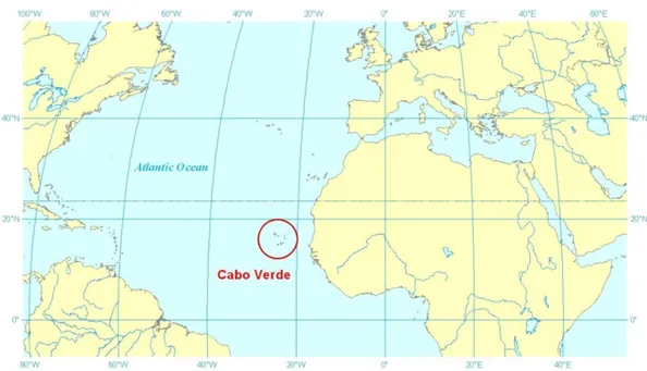
Figure 1: Localization of Cape Verde
Cape Verde is an archipelago of ten islands (nine inhabited) and five islets located in the eastern Atlantic Ocean, approximately 570 kilometres (km) from the coast of Senegal, West Africa (16N, 24W) (Figure 1).
These islands occur in two groups, the Barlavento (in the north) and Sotavento (in the south). Total land area for the archipelago is 4,564 km2.The archipelago is volcanic in origin, and is situated in the southwestern portion of the Senegalese continental shelf, on the oceanic crust.
The landscape is rugged on the younger islands (Fogo, Santo Antão, Santiago, and São Nicolau), with peaks reaching over 2,000m (highest mountain is Mount Fogo,
16 2,829 m), but relatively flat on the older islands (Maio, Sal, and Boa Vista). The degree of topographical variation is mainly related to the age of the islands and the presence of volcanoes. The major rocks are basalt and limestone, and there are deposits of salt and kaolin.
Cape Verde is on the edge of the North African arid climatic zone and has been heavily influenced throughout the last decade by the Sahelian drought. The climate is dry tropical with a strong oceanic influence that temperate thermal fluctuations. The dry season runs from December to July and the warm and wet season runs between August and November. Temperatures range between 20°C and 35°C, and average between 25°C and 29°C. Rainfall is irregular with great variability inter and intra annual, periodically the islands experience prolonged droughts. The torrential character of the rains cause heavy soil erosion and reduced water infiltration. Rainfall in most of the country ranges between 100 to 250 mm annually.
The climate is influenced by the cold current of the Canary Islands and three principal winds: the Northeast trade winds (80%), the South West monsoon (5%) and Harmattan from Est (6%) (Brochmann et al, 1997). The first is constant and blows from November to June. The second is hot and humid, irregular and unstable, blows between August and October and gives rise to rains. The third is dry wind that blows occasionally between October and June and carries large amounts of Saharan dust.
The combination of these winds with the orographic variability, locally influences the climate by creating a variety of microclimates.
17 The islands are divided into five climatic zones: Extremely arid (H1), dry (H2), semi-arid (H3), sub-humid (H4) and humid (H5) (Brochmann, et al, 1987).
Climate types H4 and H5 are on exposed slopes in the sector between N and E from the 500 meters altitude where the mists carried by trade winds determine a significant contribution in horizontal precipitation. In other sectors, the climate ranges from extremely arid to semi-arid, with the latter at higher elevations or in the watersheds.
Cape Verde's flora consists of 621 species of which 240 are indigenous and 84 endemic (Brochmann, et al., 1997).
The current vegetation is the result of significant human impact that led to the introduction of nearly two thirds of the current species and substantial changes in the ecosystem.
Much of the territory is covered by open or semi-desert herbaceous vegetation. Exotic species such as Lantana camara and Furcraea foetida become naturalized and invasive in the humid areas. Other areas are dominated by agriculture and forests of anthropic origin.
The original natural vegetation remains but in few areas of the country. In the past, it was likely represented by riparian formations of Tamarix sp. and Ficus sycomorus along the streams, by Phoenix atlantica dominating the sands dunes and savanna formations dominated by Acacia albida on the southern islands and local shrub formations dominated by Nauplius daltonii.
18 The rocky slopes were covered by Sarcostemma daltonii and humid mountain slopes by continuous shrub vegetation with emerging trees of Dracaena draco and
Sideroxylon marmulano. On semi-arid and sub-humid slopes Periploca laevigata ssp. Chevalieri occurred frequently.
In that period, it seems as if there never were true forests, as the indigenous tree species of Dracaena draco, Sideroxylon marginata, Ficus sycamorus, Tamarix
senegalensis, Acacia albida, and Phoenix atlantica lack the ability to form
continuous forest cover (Brochmann, et al., 1997).
The Cape Verdean forests are the result of afforestation programs created over past decades. The first afforestations, in order to minimize the adverse effects of ecosystem degradation, were initiated during the period of Portuguese colonization from 1930 with plantation of Eucalyptus sp. in the humid areas. Starting in 1950 onward, the introduction of new species such as Pinus canariensis, P. radiata, P.
halepensis, P. pinaster, Cupressus arizonica, C. sempervirens, C. lusitanica, Grevillea robusta, Eucalyptus camaldulensis, E. globosus, E. citriodora and E. gomphocephala
and Kaya senegalensis (Silva de Carvalho, 1994).
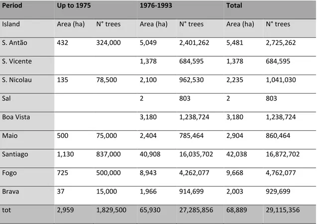
After the country's independence (1975) the afforestation was intensified (Table 3) in order to control the soil erosion, and increase the fuelwood and fodder availability.
During that period, the afforestation was concentred in the arid and semi-arid climatic zones introducing Prosopis juliflora and Prosopis pallida, Parkinsonia
aculeata and numerous species of Acacia, among which Acacia mollissima, A.cyanophilla, A. holosericea Acacia bivinosa, Acacia seleciana, Acacia Vitorie.
19 Among these species, Prosopis sp., for its ability to adapt to the soil and climate of cape Verdean islands, currently represents the 61% of wood species in terms of frequency throughout the country and 91% on Santiago Island (National Forestry Inventory 2012).
Period Up to 1975 1976-1993 Total
Island Area (ha) N° trees Area (ha) N° trees Area (ha) N° trees S. Antão 432 324,000 5,049 2,401,262 5,481 2,725,262 S. Vicente 1,378 684,595 1,378 684,595 S. Nicolau 135 78,500 2,100 962,530 2,235 1,041,030 Sal 2 803 2 803 Boa Vista 3,180 1,238,724 3,180 1,238,724 Maio 500 75,000 2,404 785,464 2,904 860,464 Santiago 1,130 837,000 40,908 16,035,702 42,038 16,872,702 Fogo 725 500,000 8,943 4,262,077 9,668 4,762,077 Brava 37 15,000 1,966 914,699 2,003 929,699 tot 2,959 1,829,500 65,930 27,285,856 68,889 29,115,356
Table 3: Afforestation of cape Verdean islands (source Direcção dos Serviços Florestais)
The study area is located in the south sector of Santiago Island, coordinates upper left 15°0´33.368"N; 23°37´42.82"W – lower right 14°56’11.818"N; 23°27’40.946"W (Figure 2).
2.1.1 STUDY AREA CHARACTERIZATION
The study area covers a surface of 14399 ha in the arid and semi-arid climatic zones representatives of xerophytics woodlands of the island.
20 Approximately 44% of the land area is covered by forests, (Figure 2); the remaining non-forested land includes non-productive areas, agriculture and urban areas.
21
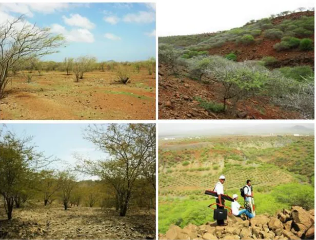
Figure 3: Aspects of the woodlands that are object of this study
These woodlands are composed by shrub-like growing species (Figure 3), Prosopis
sp. represents the 95% in frequency, of the total fifteen wood species observed.
Other species with some noticeable participation are Jatropha curcas, Acacia
nilotica, Acacia Senegal, Parkinsonia aculeata and Acacia albida. The average
canopy cover is 43%, and the mean tree density is 252 trees ha-1. The main dendrometric parameters describing the forest type in the study area, based in the field data (184 plots and 2218 trees), are reported are reported in table 4.
22 Crown area , m2 Tree Height, m Tree Biomass, Kg Mean AGB, Mg ha-1
Mean 19.29 3.52 63.21 12.701
SD 12 1.19 58 8978
CV 64% 34% 92% 71%
Table 4: Mean, standard deviation and coefficient of variation of main dendrometrics parameters describing the
forest type in the study area
Due to the adverse edaphoclimatic conditions and goat grazing, trees in the area are characterized by small dimensions, reduced crowns and low stature. When the local microclimate is more favorable, as in the streams and valleys protected from the winds, trees are bigger with denser canopies that can create continuous canopy cover. The soil is covered by grass only in the humid season (from August to November) and in the remaining months it is generally bare or covered by dried grass. These characteristic are favorable for tree crown extraction from images, since there is not overlap of canopies, the individuals can be easily detected and the bare soil is generally spectrally different and well defined from the crowns. On the other hand, the reduced crowns which are small and leafless, exhibit limited greenness and pose additional challenges to estimate correctly the sparsely existing biomass. The correct balance of these characteristics is essential in the image of processing to define an accurate method for tree crowns extraction and biomass calculation.
23 2.2 FIELD DATA
The data used as ground truth for the study are based on the fieldwork that was carried out during the first phase of the CV-NFI (2009) under the coordination of the author.
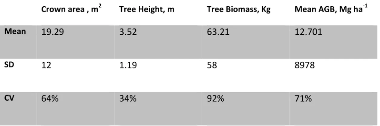
A forest non-forest map was created by manual delineation of high-resolution aerial orthophotography. During the first step, a grid of 150 m squares was overlapped to the image, and every square was classified according to the observed land cover. The minimum mapping area for each land cover class was defined at 5000m2. Following this scheme, all the squares that presenting in their centre a forest cover of > 10 % with a minimum area of 5000m2 were classified as forest and those with a forest cover >5% and <10% were classified as open forest. Only forest area is considered in the present study.
Figure 4: Detail of forest map and field plots in the study area.
A subset of the central points classified as forest was selected with a sampling intensity of 10% by means of simple random sampling without replacement
24 (SRSWOR) and surveyed in the field (figure 4). The plots were configured as circles of 500 m2.
All trees in the plot with a height more than 50 cm were mapped and described. The data collected are the following:
Tree base position, Tree species, Tree height (m), Crown projected area (based on 4 perpendiculars radius).
The field work was realized using the Field Map system. The system is composed of GNSS equipment (GPS II SXBlue), laser rangefinder/hypsometer ForestPro and electronic compass MapStar Module II, connected to a field computer with the field application (software Field-Map Data Collector). The location and navigation to the sample plots was conducted with the aid of GNSS equipment, connected to the field computer with a digital background map with the sampling plots. The position was recorded by averaging the GSSN position (at list 20 records) in open sky conditions and then completed by compass navigation until the center of the plot. Then all the trees were mapped and measured. Four pictures were taken, from the center to the four major directions (North, East, South and West) in each inventory plot. The data collected were directly stored in the database in the field computer.
Data processing was realized with Field-Map Inventory Analyst (FMIA) software in order to calculate the secondary variables such as crown width, canopy cover, aboveground biomass and the aggregation of the data from tree to plot level.
25
2.3 AERIAL PHOTOS
The imagery dataset used for this study is an aerial RGB orthophoto acquired in January 2010 with spatial resolution of 40cm (Table 5).
Radiometric & spectral resolution
Natural colour (RGB) 24-bit colour (3 x 8 bits per band) Red, blue, green
Horizontal accuracies ±3 pixels
Sensor information Analogic camera
Image width, height (pixels) 100000 x 125000
Ground sample distance (GSD) 0.4x0.4 m
Sun angle >40o
Fly altitude 3800 m
Source Geodata Air S.A.
Table 5: The characteristic of the imagery used in the study
The image was pre-processed by clipping the region of interest and converting from *.ecw to GeoTIFF format.
The Visible Atmospherically Resistant Index in the form
VARI=(Green−Red)/(Green+Red−Blue) (Gitelson et al. 2002) was calculated at this step and used as an additional band in the image processing.
26
3. M
ETHODS3.1 AGB ESTIMATION USING IMAGERY DATA
The AGB was calculated at single tree level and area based. The following scheme was applied: (1) tree crown mapping, (2) Tree crown extraction and crown projected area (CPA) calculation, (3) tree height modeling (only for single tree approach), (4) biomass calculation.
The vector layer as forestry area, field plots and crowns polygons from field measurements were organized in a GIS for the following steps.
3.1.1 TREE CROWN MAPPING
Several techniques and algorithms were tested to define the best scheme for vegetation mapping.
The processes tested as follows:
1. Image segmentation followed by a supervised classification of the segments using the k-nearest neighbour, SVM, Decision and Random Trees classifiers. 2. Image segmentation and extraction of signatures from the segments. These
segment-based training sites were used as input into pixel-based classifiers and were finally used for further classification by combining the pixel-based and the segmentbased methods. Maximum Likelihood, Fisher and K -nearest neighbor classifiers were tested in this process.
27 3. Unsupervised classification using the ISOCLUST, ISODATA and KMEANS clustering techniques followed by a threshold segmentation/classification algorithm and multiresolution segmentation based on the region grow on object algorithm (Adams 1994), (Shih and Cheng 2005).
After a number of tests we decided to apply the process nr.3 described in detail below.
The first step performed was a classification of the image using the ISOCLUST algorithm. ISOCLUST is an iterative self-organizing, unsupervised classifier based on a concept similar to the well-known ISODATA routine of Ball and Hall (1965) and cluster routines such as the H-means and K-means procedures. On the basis of a histogram, indicating the frequency of pixels that belong to each seed cluster (figure 5), a decision was made to perform the classification on 8 cluster bases.
28
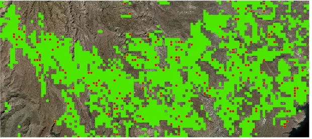
Figure 6: Result of ISOCLUST classification
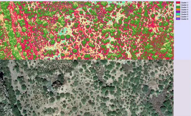
Figure 7: Tree canopy map obtained by VARI image processing
Following the classification, a visual analysis was performed in order to identify the clusters representing the tree crowns and soil (figure 6).
29 The result of ISOCLUST classification permits an initial identification of clusters representing soil and trees but some clusters are mixed between soil and crowns, avoiding a correct extraction of the canopies for biomass calculation.
Complementary the analysis of the VARI image showed good results in separating the trees from the soil (figure 7). In this case, the soil is completely excluded and the big and green canopies perfectly identified. The problem in this case is posed by the smallest and leafless crowns that are lost.
With the purpose of cleaning and separating and the mixed clusters, a process of fusion and resampling of the two images was performed. On this basis, the ISOCLUST image was reclassified assigning negatives numbers to the clusters representing soil and high positives numbers to the ones representing the canopies. The mixed clusters, that include canopies portions, shadowed areas and bright parts of canopies and soil were reclassified to intermediary values (table 6).
Cluster Nr. Description Value assigned
Cluster 1 Bright side of crowns and soil 10
Cluster 2 Soil -10
Cluster 3 Trees and some dark soil areas 20
Cluster 4 Soil -10
Cluster 5 Scattered pixel of crowns 5
Cluster 6 Light soil -10
Cluster 7 Trees and shadows 50
Cluster8 Scattered pixels of soil and crowns 3
Table 6: Description of the clusters resulting from the ISOCLUST classification and new values
30 This reclassified image was then fused with the VARI image. The fusion was realized by a sum between the two images. To amplify the difference between the negative numbers, representing the soil pixels, and positive numbers representing the tree pixels (figure 8), the VARI image was previously reclassified in the range -200 +200.
The resulting image was then reclassified to increase the difference between the soil and canopies pixels, for this, all the values between the minimum (-210) and -5 were reclassified to -10 and all the values >20 to 100. The process was followed by mean filtering with a 3 × 3 window followed by reclassification in equal intervals of 1-255. The accuracy of the result was assessed by visual interpretation over the scene on the basis of the RGB image (figure 9).
31
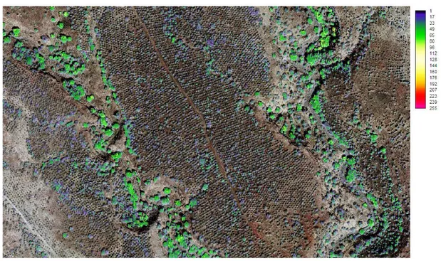
Figure 8: The VARI of a portion of the scene.
Figure 9: Overlap between the RGB and the ISOCLUST+VARI reclassified image for classification
32
3.1.2 TREE CROWN EXTRACTION AND CPA CALCULATION
Figure 10: Sequential steps of image processing from the composite RGB image (a) to the ISOCLUST
+VARI fusion (b) and threshold classification (c) and segmentation (d).
Two different approaches were followed: area based and single tree level.
Area Based:
The classified image was processed by reclassification to the values 0-1 (soil–tree respectively) with a sequence at different thresholds. The accuracy of crown
33 mapping was tuned by an iterative process. The first level was assessed by contrasting the crown map image with the RGB.
The image was then generalized, reducing the pixel size to 22.4m x22.4 m (equal to the field plot area of 500 m2), using the pixel aggregation as the contraction rule. The total CPA per pixel was then calculated.
The final tuning of the model was realized by regression analysis between the true and image retrieved CPA. During this process a sequence of decreasing threshold levels was tested and the resulting Pearson correlation coefficient and Normalized Root Mean Square Error (NRMSE) was observed in order to define the optimal threshold level (table 7).
Threshold NRMSE CPA Coeff. of Det. % AGB NRMSE biomass
15 59% 49.64% 59% 12 55% 51.41% 55% 10 51% 53.23% 51% 9 49% 54.28% 50% 7 46% 55.35% 48% 5 46% 55.35% 48%
34 Single tree approach
Figure 11: Comparison between field measured crowns (red polygons) and segments obtained by
image processing (green polygons).
The image was processed by the threshold segmentation/classification algorithm (figure 10) followed by the subsequent step of multiresolution segmentation based on the region grow on object algorithm (figure 11).
Similar to the area based approach, the first step was to define the optimum threshold by testing a sequence of decreasing values.
At the next step, different combinations of the settings, such as the scale factor, color/shape, smoothness/compactness were iteratively tested (figure 12) in order
35 to define the best combination that minimizes the RMSE of the crown area and biomass estimation.
Figure 12: Comparison between different setting of color/shape and smoothness/compactness. The
blue lines represent the results of higher compactness (1) and the red lines higher smoothness (0), the black lines represent the field plot and crowns. A) color/shape 0.5 smoothness/compactness 1; B) color/shape 0.5 smoothness/compactness 0; C) color/shape 1 smoothness/compactness 1; D color/shape 0 smooth-ness/compactness 0.
The objects were converted into vectors and processed by GIS software.
The following steps were: area calculation and selection of tree crown polygons corresponding to each field plot for model accuracy assessment. In order to minimize the edge effect, and simulate the same process of tree mapping in the
36 field, the selection of the polygons was performed using the spatial selection function “target layers features have their centroid in the source layer feature” where the target layers are the tree crowns polygons and the source layer are the field plots polygons.
3.1.3 TREE HEIGHT MODELLING
The tree height for each segment was calculated by the horizontal crown projection-height relation. The model was calculated on the basis of field data collected in 630 plots from Santiago Island for the Cape Verdean National Forest Inventory (CV-NFI) from Prosopis sp. (n=7171) (figure 13). The model is based on the equation:
Tree height = 1,2757CPA0,3683 (R² = 0.5331)
Figure 13: Relation between horizontal crown area and tree height for Prosopis sp. in Santiago island
y = 1.2757x0.3683 R² = 0.5331 0 2 4 6 8 10 12 0 50 100 150 Tr e e h e ig h t, m Crown area, m2
Crown area m
2vs Tree height m
37
3.1.4 BIOMASS CALCULATION
According to the approach as we tested, single tree and area based, the AGB was calculated in two different ways.
In the first approach and for the field data, the AGB was calculated by the allometric equations developed specifically within the CV-NFI (Cienciala et al. 2013). The study on biomass models used destructive sampling of Prosopis juliflora that was carried out on three islands, namely Santo Antão, Santiago and Maio.
The equation used is the one based on the crown width (CW) and tree height (Ht):
AGB = 1,098*EXP(-0,23+0,528*LN(Ht)+2,159*LN(CW)) (n=237 r2=0.729)
The biomass was calculated at single tree level, using as input variables the CPA, extracted from the images, and the modeled tree height. The biomass at plot level was then calculated as a sum of the individual AGB.
In the second approach, regression analysis, was used in deriving models for biomass as function of CPA. The AGB was calculated by the equation that minimizes the RMSE (figure14) using as input the total CPA of each 500m2 pixels.
38
Figure 14: Relation between tree crown area and biomass.
3.2 ACCURACY ASSESSMENT
Biomass estimates and CPA measured from field plots were used as ground truth data to evaluate predictions of biomass obtained from the models.
The validation of AGB imagery estimation models was done against allometric-based (field-measured) biomass.
Traditionally, the accuracy of forest biomass/carbon estimates is assessed by calculating the root mean square error (RMSE) and the Pearson’s correlation coefficient of the estimated and observed values (Congalton 2001; Congalton and Green 2009; Wang and Gertner 2013).
Accordingly, the accuracy of the values predicted was measured by RMSE (Equation 1) and the normalized root mean square error (NRMSE) to the mean of the observed data (Equation 2).
y = 2.6358x + 110.91 R² = 0.7014 0 500 1000 1500 2000 2500 3000 0 200 400 600 800 Image re tr iv ed C PA , m 2/p lo t
39
n
X
X
RMSE
n i obsi modeli
1 2 , ,)
(
Equation 1: RMSE obsX
RMSE
NRMSE
Equation 2: NRMSEThe relationship between the different parameters was studied by linear and power correlations and the correspondent Pearson correlation coefficient and coefficient of determination (r2).
40
4. R
ESULTS4.1 TREE CROWNS MAPPING
The visual assessment of the classification accuracy shows good results all throughout the image (fig.15); good identification of the trees is reached even for the smallest crowns and in the most complex structures.
Figure 15: The final result of tree crowns mapping in a portion of the scene.
Only some localized and well identified areas, where the soil is darker or covered by grass, was impossible to completely separate the tree crowns from the background at the selected threshold. During image processing was observed that the use of higher threshold values can increase the accuracy in the shadowed and dark areas on the contrary lower threshold where better defining the tree crowns in the and the lighter parts of the scene. Obviously in the first case, the smallest trees and bright parts of the tree crowns are lost and in the second a quick increase in the noise and incorrect classification was observed. Increased results can be reached
41 working in sub datasets divided by more homogeneous characteristics of background and tree size and by using different thresholds for each condition.
4.2 MODELS TUNING
The tuning process performed in the image processing indicated that the primarily factor influencing AGB estimation accuracy is the classification of the image, followed by the scale applied in the image segmentation for the tree crown extraction in the single tree scheme. Threshold levels above seven resulted in a rapid increase of the RMSE whereas below five there was no change detected.
Little influence was observed in the fine tuning of color/shape and smoothness/compactness settings. In the tests performed a maximum of 2% of the total NRMSE of biomass estimation was affected by setting the color/shape and smoothness/compactness parameters to extremes values. The better results were observed in middle range of values reaching the minimum RMSE with the color/shape defined at 0.3 and smoothness/compactness at 0.6.
4.3 TREE CROWN PROJECTED AREA CALCULATION
The analysis of the data exhibits the possibility of an accurate calculation of the tree crown projections with a NRMSE of 40%. Analogous results are observed in the single tree and area based approaches at plot level and original resolution (figure 16 and 17a). The generalization at 500m2 pixels, applied in the area based approach, produces a decrease of the estimation accuracy. It seems due to the resampling
42 that enhances the edge effect when comparing the circular plots data samples with square pixels.
Figure 16: Relation between observed and predicted CPA, m2 per plot (500m2), in the single tree approach. The CPA is the sum of the individual’s segments area having their centroid inside the plots
Figure 17: Relation between observed and predicted CPA, m2 per plot (500m2), in the area based approach. Figure A is the extracted CPA from the circular plots at original resolution. Figure B represents the CPA extracted from the spatialized map at 500m2 pixel resolution.
R² = 0.6689 0 100 200 300 400 500 600 700 800 0 200 400 600 800 Pr e d ic te d true RMSE 82 NRMSE 40% R² = 0.6643 0 100 200 300 400 500 600 700 0 100 200 300 400 500 600 700 Pr e d ic te d True
A ) Area based model RMSE 81 NRMSE 40% A R² = 0.5363 0 100 200 300 400 500 600 700 0 100 200 300 400 500 600 700 Pr e d ic te d True RMSE 92 NRMSE 46% B) Area based spatial