UNIVERSITY
OF TRENTO
DIPARTIMENTO DI INGEGNERIA E SCIENZA DELL’INFORMAZIONE
38050 Povo – Trento (Italy), Via Sommarive 14
http://www.disi.unitn.it
EXPLORING AND UNDERSTANDING
CITATION-BASED SCIENTIFIC METRICS
Mikalai Krapivin, Maurizio Marchese, Fabio Casati
May 2008
Exploring and Understanding Citation-based
Scientific Metrics
Mikalai Krapivin
Department of Information
Engineering and Computer Science
University of Trento, Italy
[email protected]
Maurizio Marchese
Department of Information
Engineering and Computer Science
University of Trento, Italy
[email protected]
Fabio Casati
Department of Information
Engineering and Computer Science
University of Trento, Italy
[email protected]
ABSTRACT
This paper explores citation-based metrics, how they differ in ranking papers and authors, and why. We initially take as example three main metrics that we believe significant; the standard citation count, the more and more popular h-index, and a variation we propose of PageRank applied to papers (called PaperRank), that is appealing as it mirrors proven and successful algorithms for ranking web pages. As part of analyzing them, we develop generally applicable techniques and metrics for qualitatively and quantitatively analyzing indexes that evaluate content and people, as well as for understanding the causes of their different behaviors. Finally, we extend the analysis to other popular indexes, to show whether the choice of the index has a significant effect in how papers and authors are ranked.
We put the techniques at work on a dataset of over 260K ACM papers, and discovered that the difference in ranking results is indeed very significant (even when restricting to citation-based indexes), with half of the top-ranked papers differing in a typical 20-element long search result page for papers on a given topic, and with the top researcher being ranked differently over half of the times in an average job posting with 100 applicants.
1. INTRODUCTION
The area of scientific metrics (metrics that assess the quality and quantity of scientific productions) is an emerging area of research aiming at the following two objectives: 1) measuring scientific papers, so that “good” papers can be identified and so that researchers can quickly find useful contributions when studying a given field, as opposed to browsing a sea of papers, and 2) measuring individual contributions, to determine the impact of a scientist and to help screen and identify candidates for hiring and promotions in industry and academia.
Until only 20 years ago, the number of researchers and of conferences was relatively small, and it was relatively easy to assess papers and people by looking at papers published in international journals. With small numbers, the evaluation was essentially based on looking at the paper themselves. In terms of quantitative and measurable indexes, the number of publication was the key metric (if used at all). With the explosion of the number of researchers, journals, and conferences, the “number of publications” metric progressively lost meaning. On the other hand, this same explosion increased the need for quantitative metrics at least to “filter the noise”. For example, a detailed, individual, qualitative analysis of hundreds of applications typically received today for any job postings becomes hard without quantitative measures for at least a significant preliminary filtering.
Recently, the availability of online databases and Web crawling made it possible to introduce and compute indexes based
on the number of citations of papers (citation count and its variations or aggregations, such as the impact factor and the h and g indexes [13]) to understand the impact of papers and scientists on the scientific community. More and more, Universities (including ours) are using these indexes as a way to filter or even decide how to fill positions by “plotting” candidates on charts based on several such indexes.
This paper performs an experimental study of scientific metrics (and, in particular, citation-based metrics) with the goal of 1) assessing the extent of differences and variations on the evaluation results when choosing a certain metric over another, and 2) understanding the reasons behind these differences. Besides “traditional” metrics, we also present and discuss metrics for papers and authors inspired at how the significance of Web pages is computed (essentially by considering papers as web pages, citations as links, and applying a variation of PageRank). PageRank-based metrics are emerging as important complement to citation counts as they incorporate the “weight” (the reputation or authority) of the citing paper and its density of citations (how many other papers it references) in the metric. In addition, the fact that they have been working very well for the Web suggests that they may be insightful for papers as well.
Besides the introduction of the PageRank-based index and its computation algorithm, the main contributions of this paper lie 1) in the experimental analysis of metrics, so that people and developers in “ranking” papers and people are aware of how much choosing different indexes results in different versions of the truth, and why this is the case, and 2) in the identification of a generally applicable analysis method and of a set of indicators to assess the difference between ranking algorithms for papers and people.
We performed the analysis on a dataset consisting of over 260K ACM publications. The analysis was conducted by 1) computing the various citation-based indexes; 2) analyzing the extent of the differences in ranking of papers and people depending on the metric, 3) developing “meta-indexes” whose purpose is to help explore the reasons for these differences, and 4) using these exploration indexes to derive conclusions of when and why page rank and citation measures differ and what to make of this difference. The results of the analysis are rather surprising, in that even if we restrict to citation-based indexes, the choice of the specific index rather than another changes the result of filtering and selection of papers and people about half of the times.
The structure of the paper is as follows. Related work is presented in Section 2. In section 3 we describe the dataset and in Section 4 we focus on the presentation of the main indexes for papers and for authors and on their computation for the particular dataset. The in-depth exploration of the indexes is provided in Section 5 (for papers) and section 6 (for authors), along with
comments and discussions on the results and with the introduction of the appropriate meta-indexes. Finally, the major findings of the present work are summarized in Section 7.
2. STATE OF THE ART
After the Second World War, with the increase in funding of Science and Technology (S&T) initiatives (especially by public institutions), the need for supervising and measuring the productivity of research projects, institutions, and researcher themselves became apparent [9; 10]. Scientometrics was then born as a science for measuring and analysing quantitatively science itself [7]. Nowadays, the quantitative study of S&T is a rapidly developing field, also thanks to a greater availability of information about publications in a manner that is easy to process (query, analyze).
The easiest measure to show any individual scientist’s output is the total number of publications. However, this index does not express the quality or impact of the work, as the high number of conferences and journals make it easy to publish even low quality papers.
To take quality and impact into account, the citations1 that a
paper receives emerged, in various forms, as a leading indicator. The citation concept for academic journals was proposed in the fifties by Eugene Garfield, but received the deserved attention in 1963 with the birth of the Science Citation Index (SCI) [9]. SCI was published by the Institute for Scientific Information (ISI) founded by Garfield himself in 1960 and currently known as Thomson Scientific that provides the Web of Science2
on-line commercial database. The most studied and commonly used indexes (related to SCI) are, among others [16]:
P-index: or just number of articles of author.
CC-index: number of citations excluding self-citations. CPP: or average number of citations per article.
Top 10% index: the number of papers of a person that are in the top 10% most frequently cited papers in the domain during the past 4 years.
Self-citation percentage. Career length in years.
Productivity: quantity of papers per time-unit.
Although most of the indexes are related mainly to authors, they can also be applied to measuring communities, institutions or journal, using various forms of aggregation.
In the last decade new indexes have been proposed. These indexes are rapidly gaining popularity over the more traditional citation metrics described above:
H-index, proposed by Hirsch in [13]. The H-index for an author is the maximum number h such that the author has at least h articles with h citations each. This index is widely used (including in our University), and comes in different flavors (e.g., normalized based on average number of authors of papers, on the average citations in a community, etc…). The G-index for an author is the maximum number g such
that the most cited g papers of an author collectively received g2 citations. The g index takes into account papers with very
1 a citation data is a data on references cited in footnotes or
bibliographies of scholarly research papers
2 http://scientific.thomson.com/products/wos/
high citations, which is something that is smoothed out by the h-index.
In addition, we mention below some algorithm for ranking Web pages. They are relevant as many of them have been very successful for ranking web content, and papers share some similarities with Web sites, as they can be seen as a sort of hypertext structure is papers are seen as web pages and citations are seen as links.
Hypertext-Induced Topic Selection (HITS) [14]: based on graph linkage investigation, it operates with two notions: “authority” and “hub”, where authority represents relevance of the page (graph node) to query and hub estimates the value of the node's links to other pages.
PageRank (described in more detailed in the following): a well-known and successful ranking algorithm for Web pages [3], based on net random walking probabilistic model. When modified for ranking scientific papers, it has been shown to give interesting results [5].
Hilltop [1]. This algorithm is based on the detection of "expert pages", i.e., pages that have many outgoing links (citations) and are relevant to a topic. Pages that are linked by expert ones have better rank.
In our work we adopt a variation of PageRank as one of the main indexes used for the analysis of differences among indexes. The intuition behind PageRank is that a web page is important if several other important web pages point to it. Correspondingly, PageRank is based on a mutual reinforcement between pages: the importance of a certain page influences and is being influenced by the importance of some other pages. From a computational point of view, PageRank is a statistical algorithm: it uses a relatively simple model of "Random Surfer" [3] to determine the probability to visit a particular web page. Since random browsing through a graph is a stochastic Markov process, the model is fully described by Markov chain stochastic matrix. The most intriguing question about PageRank is how to compute one for a dataset as huge as the web.
The inventors of PageRank, Brin and Page, proposed a quite effective polynomial convergence method [3], similar to the Jacobi methods. Since then, a significant amount of research has been done in the exploration of the meaning of PageRank and proposals for different computation procedures [2] [6] [5]. When the attention is shifted from web pages to scientific citations, the properties of the citation graph – mainly its sparseness – has been used to simplify the computational problem [20].
In our work, we have based our computations on a variation of Page Rank (called Paper Rank) for ranking scholarly documents explained in detail in Section 4. From a computational perspective, the difference is that the algorithm we propose exploits the fact that in citations, unlike in web links, cycles are very rare.
In terms of comparison among scientific metrics for determining the difference in the ranking results they generate (and methods for evaluating such differences), there is no prior art to the best of our knowledge.
3. DATA SET DESCRIPTION AND DATA
PREPROCESSING
The starting point for our analysis is a dataset of 266788 papers published in ACM conferences or journals, and authored by
244782 different authors. The dataset was available as XML documents that for each paper describes information such as authors, title, year of publication, journal, classification and keywords (for some of the papers), journal volume and pages, and citations. A sample of the dataset format is available at the companion web page mentioned earlier.
The set is biased in terms of citation information. For any given paper in the set, we have all its references (outgoing citations), but we only have citations to it (incoming citations) from other papers in the dataset, and hence from ACM papers. To remove the bias (to the possible extent), we disregard references to non-ACM papers. In other words, we assume that the world, for our citation analysis, only consists of ACM papers. Although we have no measurable evidence, given that we are comparing citation-based metrics we believe that the restriction to an “ACM world” does not change the qualitative results of the analysis. Including references to non-ACM papers would instead unfairly lower the measure for Paper Rank since, as we will show, Paper Rank is based on both incoming and outgoing citations.
This being said, we also observe that the quality of the chosen dataset is very high. The majority of papers have been processed manually during the publishing process and all author’s names have been disambiguated by humans. This is crucial since systems like Google Scholar3 or Citeseer4 contain errors in the
disambiguation of authors names and citations. In fact, both Goodle Scholar or other autonomous digital libraries like Citeseer or Rexa5 use machine learning-based unsupervised techniques to
disambiguate the information and are prone to introduce mistakes. A preliminary study of these errors in Google Scholar is presented in [19]. Besides disambiguation errors, crawled information may include spurious types of documents like deliverables, reports, white papers, etc. Indeed, Scholar includes in its statistics the citations coming from project deliverables or even curricula vitae, which are not commonly considered to be academically meaningful citations. Thus, although incomplete, the ACM dataset has a high level of quality in particular in respect to authors and citations.
The full citation graph of the ACM dataset has 951961 citations, with an average of 3.6 outgoing citations per paper (references to other ACM papers). Figure 1 shows instead how many papers have a given (incoming) citation count (hereafter called CC). As expected, there is a very large number of papers with low, near-zero citations and a few papers with a high number of citations.
3http://scholar.google.com 4 http://citeseer.ist.psu.edu/ 5 http://rexa.info/
Figure 1. Distribution of papers by Citation Count.
The years of publication of the papers in the dataset vary from 1950 to 2005 with most emphasis on the recent two decades due to the increase in the number of publications.
4. PAPER RANK AND PR-HIRSCH
This section describes the Paper Rank (PR) algorithm for ranking papers and the corresponding measure (PR-Hirsch) for ranking authors.
4.1 Page Rank outline
The original Page Rank algorithm [3] ranks the nodes of a directed graph with N vertices. The rank of a node is determined by the following recursive formula, where S(j) is the quantity of outgoing links from a node Pj. are just sequence
numbers and D is the set of nodes such that there is a path in the graph from them to node i.
}
..
1
{
,
j
n
i
∈
∑
∈ ≠=
j D j i j ij
S
P
P
)
(
(1)The formula can be seen in matrix form and the computation can be rewritten as an eigenvector problem:
r
r
=
A
⋅
r
r
(2) where A is the transition matrix, or stochastic Markov matrix.This consideration exposes several potential problems in rank computation as discussed in [2][15]. One of them is the presence of the nodes which link to other nodes but are not linked by other nodes, called dangling nodes. In this case, equation (2) may have no unique solution, or it may have no solution at all (it will lead to zero-rows occurrence in the transition matrix and uncertainty of the rank of the dangling nodes). Such problem may be resolved with the introduction of a dump-factor d. The damp (or decay) factor is a positive double number 0 < d < 1:
N
d
j
S
P
d
P
D j j i j i=
−
⋅
∑
+
∈ ≠(
)
)
1
(
(3)The damp factor was proposed by the PageRank inventors, Page and Brin. In their publication [3], Page and Brin give a very simple intuitive justification for the PageRank algorithm: they introduce the notion of ‘random surfer‘. Since in the specific case of web pages graph, the equivalent stochastic Markov matrix can be described as browsing through the links, we may imagine a ‘surfer’ who makes random paths through the links. When the surfer has a choice of where to go, it chooses randomly the next page to visit among the possible linked pages The damp factor models the fact that surfers at some point get bored of following links and stop (or begin another surf session). The damp factor therefore also reduces the probability of surfers ending up in dangling nodes, especially if the graph is densely connected and dangling nodes are few.
The damp factor helps to achieve two goals at once: 1) faster convergence using iterative computational methods, 2) ability to solve the equation, since all the nodes must have al least d/N Page Rank even if they are not cited at all.
4.2 Paper Rank
PageRank has been very successful in ranking web pages, essentially considering the reputation of the web page referring to a given page, and the outgoing link density (pages P linked by pages L where L has few outgoing links are considered more important than pages P cited by pages L where L has many outgoing links). Paper Rank (PR) applies page rank to papers by considering papers as web pages and citations as links, and hence trying to consider not only citations when ranking papers, but also taking into account the rank of the citing paper and the density of outgoing citations from the citing paper.
From a computation perspective, PR is different from Page Rank in that loops are very rare, almost inexistent. Situations with loop where a paper A cites a paper B and B cites A are possible when authors exchange their working versions and cite papers not yet published but accepted for publication. In our dataset, we have removed these few loops (around 200 loops in our set). This means that the damp factor is no longer needed to calculate PR. Because of the above analysis, we can compute PR directly according to the formula (1).
Furthermore, considering that a citation graph has N>>1 nodes (papers), each paper may potentially have from 1 to N-1 inbound links and the same quantity of outgoing ones. However, in practice citation graphs are extremely sparse, (articles normally have from 5 to 20 references) and this impact the speed of the computation of PR.
However, also in this case the matrix form of the problem (i.e. formula (2)) may have no solution, now because of initial nodes (nodes who are cited but do not cite). To avoid this problem we slightly transform initial problem assigning a rank value equal to 1 to all initial nodes, and resetting it to zero at the end of the computation (as we want to emphasize that papers who are never cited have a null paper rank). Now the problem became solvable and the Markov matrix may be easily brought to the diagonal form. We used fast and scalable recursive algorithm for calculating Paper Rank, which corresponds to the slightly different equation:
r
r
=
A
⋅
r
r
+
r
r
0 (4)4.3 PR-Hirsch
One of the most widely used indexes related to author is the H-index proposed by Jorge Hirsch in 2004 [13] and presented
earlier. The H-index tries to value consistency in reputation: it is not important to have many papers, or many citations, but many papers with many citations.
We propose to apply a similar concept to measure authors based on PR. However, we cannot just say that PRH is the maximum number q such that an author has q papers with rank q or greater. This is because while for H-index it may be reasonable to compare number of papers with number of citations the papers have, for PRH this may not make sense as PR is for ranking, not to assign a meaningful absolute number to a paper. The fact that a paper has a CC of 45 is telling us something we can easily understand (and correspondingly we can understand the H-index), while the fact that a paper has a PR of 6.34 or 0.55 has little “physical meaning”.
In order to define a PR-based Hirsch index, we therefore rescale PR so that it gets to a value that can be meaningfully compared with the number of papers. Let’s consider in some detail our set: we have a graph with N nodes (vertices) and n citations (edges). Each i-th node has PR equal to Pi, that expresses
the probability for a random surfer to visit a node, as in the Page Rank algorithm. So let’s assume that we run exactly n surfers (equal to quantity of citations), and calculate the most probable quantity of surfers who visited node i. If the probability to visit the node i for one surfer is pi, expectation value Qi for n surfers to
visit the node i will be pi • n, which is most probable quantity of
surfers, who visited node i. We sum probabilities since all surfers are independent. To be precise we should first normalize PR for each node according to full probability condition:
∑
=
1
i i
p
. Ifthe total sum of all PRs equals to M, the expected value for n surfers is as follows:
M
n
P
Q
i=
i (4) Where Pi is a Paper Rank of the paper i, n/M is the constant≈5.9169 for our citation graph. So in other words we rescale PR to make it comparable with the quantity of citations. Indeed, Qi is the
most probable quantity of surfers who visited a specific paper i, whereas to compute Hirsch index we use quantity of citations for the paper i. It is interesting to compare the ranges of Q and citation count (see Table 1).
Following the definition of H-index and the previous discussion, we define PR-Hirsch as the maximum integer number h such that an author has at least h papers with Q value (i.e. rescaled PR following equation (4)) equal or greater than h.
Table 1. Comparison of citation count and random surfers count mathematical expectation values for all papers in graph.
Average Q Maximum
Q Average CC
Maximum CC
3.57 1326.77 3.57 1736
5. EXPLORING PAPER METRICS
This section explores the extent of the differences between paper metrics PR and CC when ranking papers, and their causes. As part of the analysis we introduce concepts and indexes that go beyond the PR vs CC analysis, and that are generally applicable to
understanding the effects and implications of using a certain index rather than another for assessing papers’ value.
5.1 Plotting the difference
The obvious approach to exploring the effect of using PR vs CC in evaluating papers would consist in plotting these values for the different papers. Then, the density of points that have a high CC and low PR (or vice versa) would provide an indication of how often these measures can give different quality indication for a paper. This leads however to charts difficult to read in many ways: first, points overlap (many papers have the same CC, or the same PR, or both). Second, it is hard to get a qualitative indication of what is “high” and “low” CC or PR. Hence, we took the approach of dividing the CC and PR axis in bands.
Banding is also non-trivial. Ideally we would have split the axes into 10 (or 100) bands, e.g., putting in the first band the top 10% (top 1%) of the papers based on the metric, to give qualitative indications so that the presence of many papers in the corners of the chart would denote a high divergence. However the overlap problem would remain, and it would distort the charts in a significant way since the measures are discrete. For example the number of papers with 0 citations is well above 10%. If we neglect this issue and still divide in bands of equal size (number of papers), papers with the same measure would end up in different bands. This gives a very strong biasing in the chart (examples are provided in the companion page).
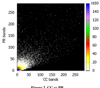
Finally, the approach we took (Figure 2) is to divide the X-axis in bands where each band corresponds to a different citation count measure. With this separation we built 290 different bands, since there are 290 different values for CC (even if there are papers with much higher CC, there are only 290 different CC values in the set). For the Y-axis we leverage mirrored banding, i.e., the Y-axis is divided into as many bands as the X-axis, also in growing values of PR. Each Y band contains the same number of papers as X (in other words, the vertical rectangle corresponding to band i in the X axis contains the same number of papers qi as
the horizontal rectangle corresponding to band i of the Y-axis). We call a point in this chart as a square, and each square can contain zero, one, or many papers.
The reasoning behind the use of mirrored banding is that this chart emphasizes divergence as distance from the diagonal (at an extreme, plotting a metric against itself with mirrored banding would only put papers in the diagonal). Since the overlap in PR values is minimal (there are thousands of different values of PR and very few papers with the same PR values, most of which having very low CC and very low PR, and hence uninteresting), it does not affect in any qualitatively meaningful way the banding of the Y-axis.
Figure 2. CC vs PR.
X axis plots CC bands, Y axis plots PR mirror-banded by CC. The color corresponds to the number of papers within a band.
(For actual values of PR and CC for each band see Table 2) Table 2 gives an indication of the actual citation and PR values for the different bands.
Table 2. Mapping of band number to the actual value of CC or average actual value for PR.
Number of band both for CC and PR CC PR 50 50 6.23 100 100 14.74 150 151 26.57 200 213 38.82 250 326 58.86 280 632 113.09 290 1736 224.12
The chart in Figure 2 shows a very significant number of papers with a low CC but a very high PR. These are the white dots (a white color corresponds to one paper). Notice that while for some papers the divergence is extreme (top left) and immediately noticeable, there is a broad range of papers for which the difference is still very significant from a practical perspective. Indeed, the very dense area (bands 1-50) includes many excellent papers (CC numbers of around 40 are high, and even more considering that we only have citations from ACM papers). Even in that area, there are many papers for which the band numbers differ significantly if they are ranked by CC or PR.
To give a quantitative indication of the difference, Table 3 below shows how far apart are the papers from the diagonal. The farther away the papers, the more the impact of choosing an index over another for the evaluation of that paper.
Table 3. Deviation of papers around main diagonal. Distance in bands
from the diagonal
% of papers with this distance
0 36.83 1 24.30 2 13.02 3 5.76 4 5.43 5 2.50 6 1.70 7 1.34 8 1.86 9 1.57 10 0.79 ≥11 4.89
The mean value for the distance from the main diagonal is 3.0 bands, while the standard deviation is 3.4. This deviation from the average is rather significant, i.e. in average the papers are dispersed through 3 bands around main diagonal.
In the subsequent discussion, we will qualitatively refer to papers with high PR and high CC as popular gems, to paper with high PR and low CC as hidden gems, to papers with low PR and high CC as popular papers, and to papers with low CC and PR as dormant papers (which is an optimistic term, on the assumption that they are going to be noticed sometime in the future).
5.2 Divergence
The plots and table above are an attempt to see the difference among metrics, but it is hard from them to understand what this practically means. We next try to quantitatively assess the difference in terms of concrete effects of using a metric over another for what metrics are effectively used, that is, ranking and selection. Assume we are searching the Web for papers on a certain topic or containing certain words in the title or text. We need a way to sort results, and typically people would look at the top result, or at the top 10 or 20 results, disregarding the rest. Hence, the key metric to understand divergence of the two indexes is how often, on average, the top t results would contain different papers, with significant values for t =1, 10, 20.
Specifically, we introduce a metric called divergence, which quantitatively measures the impact of using one scientometric index versus the other. Consider two metrics M1 and M2 and a set
of elements (e.g., of papers) S. From this set S, we take a subset n of elements, randomly selected. For example, we take the papers related to a certain topic. These n papers are ranked, in two different rankings, according to two metrics M1 and M2, and we
consider the top t elements. We call divergence of the two metrics, DivM1,M2 (t,n,S), the average number of elements that
differ between the two sets (or, t minus the number of elements that are equal). For example, if S is our set of ACM papers, and n are 1000 randomly selected papers (say, the papers related to a certain topic or satisfying certain search criteria), DivCC,PR
(20,1000,S) measures the average number of different papers that we would get in the typical 20-item long search results page. We measured the divergence experimentally for CC and PR, obtaining the results in the table below. As a particular case, DivM1,M2 (1,n,S)
measures how often does the top paper differs with the two indexes.
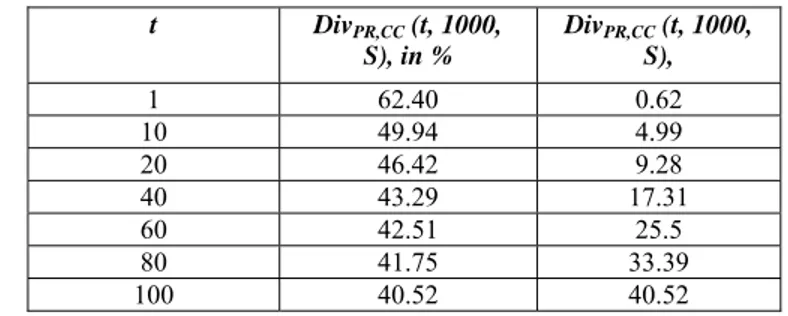
Table 4. Experimentally measured divergence for the set of ACM papers. t DivPR,CC (t, 1000, S), in % DivPR,CC (t, 1000, S), 1 62.40 0.62 10 49.94 4.99 20 46.42 9.28 40 43.29 17.31 60 42.51 25.5 80 41.75 33.39 100 40.52 40.52 The table is quite indicative of the difference, and much
more explicit than the plots or other evaluation measures described above. In particular, the table shows that more than almost 2/3 of the times, the top ranked paper differs with the two metrics. Furthermore, and perhaps even more significantly, for the traditional 20-element search result page, nearly half of the paper would be different based on the metric used. This means that the choice of metric is very significant for any practical purposes, and that a complete search approach should use both metrics (provided that they are both considered meaningful ways to measure a paper). In general we believe that divergence is a very effective way to assess the difference of indexes, besides the specifics of CC and PR. We will also see the same index on authors, and the impact that index selection can therefore have on people’s careers.
Details on the experiments for producing these results and the number of measures executed are reported in the companion web page.
5.3 Understanding the differences
We now try to understand why the two metrics differ. To this end, we separate the two factors that contribute to PR, see equation (1): the PR measure of the citing papers and the number of outgoing links of the citing papers.
To understand the impact of the weight, we consider for each paper P the weight of the papers citing it (we call this the potential weight, as it is the PR that the paper would have if all the citing papers P only cited P). We then plot (Figure 3) the average potential weight for the papers in a given square (intersection of a CC and a PR band) in the banded chart.
The estimation of the impact of outgoing links can be done in various ways. For example, we can take the same approach as for the weight and compute a double average over the outgoing links (for each paper P, compute the average number of outgoing links of the set C(P) of papers citing P, and then average them for all papers of a square in the CC vs PR chart). This is useful but suffers from the problem that if some papers (maybe “meaningless” paper with very low PR, possibly zero) have a very high number of outgoing links, they may lead us to believe that such high number of links may be the cause for a low PR value for a paper, but this is not the case (the paper is only loosing very few PR points, possibly even zero, due to these outgoing links). A high value of this measure therefore is not necessarily indicative of the number of outgoing links being a factor in low values of PR.
Figure 3. Average potential weight for all papers in a square
The color in the Z-axis denotes the weight Figure 4. Average dispersed weight for all papers in a square The color in the Z-axis denotes the weight
X axis plots CC bands, Y axis plots PR mirror-banded by CC X axis plots CC bands, Y axis plots PR mirror-banded by CC
A more meaningful approach is to measure the HOC index
for each paper P, defined as the maximum number h such that P is cited by at least h papers, each having at least h outgoing links. HOC stands for Hirsch for outgoing citation, where the reference to Hirsch is because the way it is defined resembles the Hirsch index for papers. Plotting the average HOC for all papers in a square gives us a better indication of the overall impact of outgoing links on a paper PR because it smoothes the effect of a few papers having a very high number of outgoing links. Again, examples of these plots can be found in the companion web page.
This measure is useful but does not take into account the fact that what we really want to see when examining the effect of outgoing links from citing paper is the “weight dispersion”, that is, how much weight of the incoming papers (i.e., how much potential weight) is dispersed through other papers as opposed to being transmitted to P. This is really the measure of the “damage” that outgoing links do to a Paper Rank. We compute the dispersed weight index for a paper P (DW(P)) as the sum of the PR of the citing papers C(P) (that is, the potential weight of P) divided by the PR of P (the actual weight). Figure 4 plots the average dispersed weight for each square, as usual by CC and PR. The dark area in the bottom right corner is because there are no papers there.
Figure 5. "Gem" and "popular paper" relative positions.
The specific gem is the paper Computer system for inference execution and data retrieval, by R. E. Levien and M. E. Maron, 1967. This paper has 14 citations in our ACM-only dataset (Google Scholar shows 24 citations for the same paper). The PR of this “hidden gem” is 116.1, which is a very high result: only 9 papers have a greater rank. Let’s go deep inside the graph to see how this could happen.
These two charts very clearly tell us that outgoing links are the dominant effect for the divergence between CC and PR. Papers having a high CC and low PR have a very high weight dispersion, while papers with high PR and low CC are very focused and able to capture nearly all potential weight. The potential weight chart (Figure 3) also tends to give higher numbers for higher PR papers but the distribution is much more uniform in the sense that there are papers in the diagonal or even below the diagonal and going from the top left to the bottom right the values do changes but not in a significant way (especially when compared to the weight dispersion chart).
Figure 6 shows all the incoming citations for this paper up to two levels in the citation graph. The paper in the center is our “gem”, and this is because it is cited by an heavyweight paper that also has little dispersion: it cites only two papers.
We observe that this also means that in some cases a pure PR may not be robust, meaning, the fact that our gem is cited by a heavyweight paper may be considered a matter of “luck” or a matter of great merit, as a highly respected “giant” is citing it. Again, discussing quality of indexes and which is “better” or “worse” is outside our analysis scope, as is the suggestion for the many variations of PR that could make it robust.
To see the difference concretely on a couple of example, we take a “hidden gem” and a “popular paper”, see Figure 5.
Figure 6. One of the “hidden gem” in the dataset, paper of E. Levien and M. E. Maron (in the center). Arrows refer to incoming citations. The digits near the papers refer to the quantity of outgoing links.
We now consider a paper in the bottom of the CC vs PR plot, a paper with high number of citations but relatively low PR. The corresponding citation graph is shown in Figure 7. This paper has 55 citations in our ACM dataset (158 citations in Google Scholar) and a relatively poor PR of 1.07. This result is not particularly bad, but it is much worse than other papers with similar number of citations. There are 17143 papers in the dataset that have grater Paper Rank and just 1394 papers with better citation count. Comparing with papers in the same CC and PR band, this paper has a weight dispersion factor that is over twice that of papers in the same CC band and three times the one of papers in the same PR band, which explain why the increased popularity with respect to papers in the same PR band did not correspond to a higher PR.
As a final comment, we observe that very interestingly there are papers with very low CC and very high PR, but much less papers – almost none - with very high CC and very low PR. If we follow the dispersion plot this is natural, as it would assume that the dispersed weight should be unrealistically high (many papers with hundreds of citations) which does not happen in practice, while it is possible to have “heavyweight” papers with very few citations that make the presence of paper gems (papers in the top left part) possible.
However, we believe that the absence of papers in the bottom right part and, more in general, the skew of the plot in Figure 2 towards the upper left is indicative of a “popularity bias”. In the ideal case, an author A would read all work related to a certain paper P and then decide which papers to reference. In this case, citations are a very meaningful measure (especially if they are positive citations, as in the motto “standing on the shoulders of giants”). However this is impossible in practice, as nobody can read such a vast amount of papers. What happens instead is that author A can only select among the papers she “stumbles upon”, either because they are cited by other papers or because they are returned first in search results (again often a result of high citation count) or because they are published in important venues. In any event, it is reasonable to assume that authors tend to stumble upon papers that are cited more often, and therefore these papers have a higher chance of being cited than the “hidden gems”, even if maybe they do not necessarily have the same quality. We believe that it is for this reason that over time, once a paper increases with citation count, it necessarily increases with the weight, while gems may remain “hidden” over time. A detailed study of this aspect (and of the proper techniques for studying it) is part of our future work.
6. EXPLORING AUTHOR METRICS
6.1 Plotting the difference
We now perform a similar analysis on authors rather than papers. For this, we initially consider PRH and Hirsch as main metrics, and then extend to other metrics. The plot to visualize the differences (Figure 8) is similar in spirit to the one for CC vs PR. The X-axis has Hirsch values, while the Y-axis has PRH values. A first observation is that applying “Hirsching” to CC and PR to get H-index and PRH smoothes the differences, so we do not have points that are closer to the top left and bottom right corners. This could only happen, for example, if one author had many papers that are hidden gems.
Figure 8. The gradient of Hirch and PRHirch in log scale. Author’s density is plotted with colors: authors’ number goes
from 1 to 149170 of authors per square. PR-Hirch has been rounded.
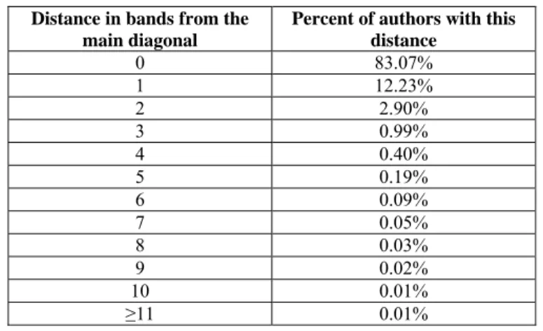
Since the authors with low Hirsch and PRH are dominant, a log scale was used plotting Figure 6. This increased similarity is also shown in Table 5, where many papers are on the diagonal (this is also due to the fact that we have a much smaller number of squares in this chart). The mean distance from the diagonal is 0.25 bands, while the standard deviation is 0.42 bands.
Interestingly, as we will see, though at first look the differences seem less significant, the impact of using one rather than the other index is major.
Table 5. Deviation of authors around main diagonal Distance in bands from the
main diagonal
Percent of authors with this distance 0 83.07% 1 12.23% 2 2.90% 3 0.99% 4 0.40% 5 0.19% 6 0.09% 7 0.05% 8 0.03% 9 0.02% 10 0.01% ≥11 0.01%
6.2 Divergence
The same measure of divergence described for papers can be computed for authors. The only difference is that now the set S is a set of authors, and that the indexes are H-index and PRH instead of CC and PR. We also compute it for n=100, as the experiment we believe it is meaningful here is to consider replies to a typical job posting for academia or a research lab, generating, we assume, around 100 applications. (Statistics for other values of n are reported in the companion web page).
Table 6. Divergence between PRH and H, n=100. t DivPRH,H(t) 1 59.3% 5 50.04% 10 46.13% 20 43.47%
Although nobody would only make a decision based on indexes, they are used more and more to filter applications and to make a decision in case of close calls or disagreements in the interview committees. The table tells us that almost two third of the times, the top candidate would differ. Furthermore, if we were to filter candidates (e.g., restrict to the top 20), nearly half of the candidates passing the cutoff would be different based on the index used. This fact emphasizes once again that index selection, even in the case of both indexes based on citations, is key to determining the result obtained, be them searching for papers or hiring/promotion of employees. Notice also that we have been only looking at differences in the elements in the result set. Even more are the cases where the ranking of elements differ, even when the t elements are the same.
Another interesting aspect is that the divergence is so high even if the plot and Table 5 show values around the diagonal. This is because most of the authors have a very low H and PRH (these accounts for most of the reasons why authors are on average on the diagonal). However, and this can also be seen in the plot, when we go to higher value of H and PRH, numbers are lower and the distribution is more uniform, in the sense that there are authors also relatively far away from the diagonal (see the softer colors and the distributions also far from the diagonal towards the top-right quadrant of Figure 8). Incidentally, we believe that this confirms the quality of divergence as a metric in terms of concretely emphasizing the fact that the choice of index, even among citation-based ones, has a decisive effect on the result.
We omit here the section on “understanding the difference” as here it is obvious and descends from the difference between CC and PR, described earlier and used as the basis for PRH and Hirsch respectively.
6.3 Divergence between other indexes
The discussion above has focused on PRH vs H. We now extend the same analysis to other indexes. The table below shows a comparison for PRH, H, G index, and the total citation count for an author (the sum of all citations for the paper by an author, denoted as TCC in the table).
Table 7. Divergence for the different indexes in %, n=100 (for simplicity the Div () notation is omitted).
t PRH vs G PRH vs TCC H vs TCC H vs G G vs TCC 1 56.3 56.4 38.2 34.6 29.9 5 45.66 46.38 29.48 25.58 23.84 10 43.05 43.03 27.9 22.94 22.95 20 41.3 41.66 27.63 21.70 22.62
The first lesson we learn from the table is that no two indexes are strongly correlated. The higher correlation is between G and the total citation count, and we still get the top choice different in one out of four cases. The other interesting aspect is that PRH and
H are the pair with the highest divergence, which makes them the two ideal indexes to be used (in case one decides to adopt only two indexes).
7. CONCLUSIONS AND FUTURE WORK
This paper has explored and tried to understand and explain the differences among citation-based indexes. In particular, we have focused on a variation of Page Rank algorithm specifically design for ranking papers – that we have named Paper Rank - and compared it to the standard citation count index. Moreover, we have analyzed related indexes for authors, in particular the Paper Rank Hirsch–index and the commonly-used H-index. We have explored in details the impact they can have in ranking and selecting both papers and authors. The following are the main findings of this paper:1. PR and CC are quite different metrics for ranking papers. A typical search would return half of the times different results. 2. The main factor contributing to the difference is weight
dispersion, that is, how much weight of incoming papers is dispersed through other papers as opposed to being transmitted to a particular paper.
3. For authors, the difference between PRH and H is again very significant, and index selection is likely to have a strong impact on how people are ranked based on the different indexes. Two thirds of the times the top candidate is different, in an average application/selection process as estimated by the divergence.
4. An analogous exploration of divergence between several citation-based indexes reveal that all of them are different in ranking papers, with g-index and total citation count being the most similar.
In addition to the findings, we believe that:
1. Divergence can be a very useful and generally applicable metric, not only for comparing citation-based indexes, but also for comparing any two ranking algorithms based on practical impact (results).
2. There are a significant number of “hidden gems” while there are very few “popular papers” (non gem). The working hypothesis for this fact (to be verified) is that this is due to citation bias driven by a “popularity bias” embedded in the author’s citation practices, i.e. authors tend to stumble upon papers that are cited more often, and therefore these papers have a higher chance of being cited
The exploration of the citation bias hypothesis is our immediate future research, along with the extension of our dataset to a more complete coverage of the citation graph, to analyze the its possible influence on the different indexes.
8. ACKNOWLEDGMENTS
We acknowledge Professor C. Lee Giles6, for sharing of
meta-information about papers, proceedings and books. The citation graph was built based on these metadata. Computations and
experiments have been done in collaboration with Andrei Yadrantsau7 who we also want to acknowledge.
9. REFERENCES
[1] Bharat K. and Mihaila, G. A.. When experts agree: Using non-affiliated experts to rank popular topics. In Proceedings of the Tenth International World Wide Web Conference, 2001. http://citeseer.ist.psu.edu/bharat01when.html [2] Bianchini, M. Gori M., and Scarselli, F.Inside PageRank,
ACM Transactions on Internet Technology, Vol. 5, No. 1, February 2005.
[3] Brin,S. , Page, L. The anatomy of a large-scale hypertextual Web search engine, Computer Networks and ISDN Systems Volume 30, Issues 1-7, Elsevier, 1998, Pages 107-117 [4] Brookes, B.C. “Bradford’s Law and the Bibliography of
Science”, Nature, 224(5223), 953-956, 1969.
[5] Chen, P. Xie, H. Maslov, S. Redner, S. Finding Scientific Gems with Google, Journal of Informetrics, Elsevier, (2007).
[6] Del Corso, G. M. Gull A., and Romani,F. Fast PageRank Computation via a Sparse Linear System, Internet Mathematics Vol. 2, No. 3: 251-273, August 31, 2005. [7] Derek deSolla Price, Little Science - Big Science, Columbia
Univ. Press, New York, (1963)
[8] Diligenti M., Marco Gori, M. Maggini, M. Web Page Scoring Systems for Horizontal and Vertical Search,
World
Wide Web Conference 2002,
Honolulu, Hawaii, USA, May 7-11, 2002.[9] Garfield, E. Citation Indexing, ISI Press, 1979.
[10] Garfield, E. The Agony and the Ecstasy - The History and Meaning of the Journal Impact Factor, International Congress on Peer Review And Biomedical Publication, Chicago, 2005.
[11] Glänzel, W. Bibliometrics as a research field, A course on theory and application of bibliometric indicators, Magyar Tudományos Akadémia, Course Handouts
http://www.norslis.net/2004/Bib_Module_KUL.pdf , (2003) [12] Glänzel, W. U. Schmoch, U. Handbook of Quantitative
Science and Technology Research, ed. by H.F. Moed, Kluwer Academic Publishers, 2004.
[13] Hirsch, Jorge E., An index to quantify an individual's scientific research output, Proceedings of the National Academy of Sciences, 102(46):16569-16572, November 15, (2005)
[14] Kleinberg J., Authoritative sources in a hyperlinked environment. In Proc. Ninth Ann. ACM-SIAM Symp. Discrete Algorithms, pages 668-677, ACM Press, New York, (1998)
[15] Langville A. N. and Meyer C. D., Deeper Inside PageRank, Internet Mathematics Vol. 1, No. 3: 335-380, 2004. [16] Moed, H.F. Citation Analysis in Research Evaluation,
Springer, (2005)
7 Belarussian State University, Minsk, Belarus
[17] Noyons, E. C. M. and van Raan, A. F. J. Monitoring scientific developments from a dynamic perspective: self-organized structuring to map neural network research. Journal of the American Society for Information Science, 49(1), pag.68-81, (1998)
[18] Pritchard A., Statistical bibliography or bibliometrics?, Journal of Documentation 24, 348-349, (1969)
[19] Scrinzi, Roberto, Sviluppo di un tool per l’esplorazione semi-automatica all’interno del servizio di Google Scholar, Thesis (in Italian), University of Trento, 2008.
[20] Sun Y. and Giles, C. Lee Popularity Weighted Ranking for Academic Digital Libraries, 605-612, 29th European Conference on IR Research, ECIR 2007, pag. 605-612, Rome, Italy.
[21] Zipf, G. K., Human Behavior and the Principle of Least Effort. Addison-Wesley, (1949).