Technical Report CoSBi 02/2006
The π-calculus with biological transactions
Federica Ciocchetta University of Trento [email protected]
Corrado Priami
The Microsoft Research - University of Trento Centre for Computational and Systems Biology
The π-calculus with biological transactions
Federica Ciocchetta University of Trento [email protected]
Corrado Priami
The Microsoft Research - University of Trento Centre for Computational and Systems Biology
Abstract
In this work we extend the π-calculus with a simple class of trans-actions, suitable to model multi-reactant, multi-product chemical re-actions. Some examples are reported to validate our extension.
1
Introduction
In the recent years, process algebras have been widely applied to model biological models [14, 11, 13, 16, 10, 6]. One of the most used process algebras in this field is the π-calculus [9], a formal language originally de-veloped for specifying concurrent computational systems. In such systems, multiple processes interact each other by synchronized pair-wise communi-cation on complementary channels and modify each other by transmitting channel from one process to another. In using the π-calculus for model-ing biological reactions, any interaction (for instance the transformation of one molecule into another one, the formation of a complex, ...) is repre-sented as a (synchronous) communication between two biological entities. A problem arises when reactions with more than two reactants are consid-ered. These reactions are rare in nature, but are often used in biological models as abstractions of complex phenomena. Generally, they represent sequence of elementary steps, whose details are unknown or not important. A possible approach to deal with these reactions is to decompose them into a sequence of two-reactant reactions. For instance, the three-reactant re-action R1 + R2 + R3 → P may be decomposed into the two elementary
reactions R1+ R2 → complex(R1, R2) and complex(R1, R2) + R3→ P . The
new element complex(R1, R2) represents the intermediate complex of the two reactants R1 and R2. Following this approach, some problems arise.
First, different orders of reactants are possible and there are n!2 ways to decompose a reaction, where n is the number of reactants (and modifiers). Furthermore, it can happen that after the formation of the intermediate complex, the third reactant misses, leading to a deadlock. A possible way to solve this problem is to consider the first reaction as reversible (i.e.
R1 + R2 ↔ complex(R1, R2)), but this solution can lead to undesired be-haviors.
Here a different approach is adopted. We propose to introduce trans-actions to model complex retrans-actions. Generally speaking, a transaction is a component of a distributed system which must be executed as if were a single atomic action. It should not be interrupted at intermediate steps and satisfies safety and failure properties. They are used to define traditional transactions in databases or composition of subtasks in web service technolo-gies. Recently there are several attempts to model transactions formally by using process algebras [1, 7, 3]. In [1] the πt-calculus is presented: it is an extended version of the asynchronous π-calculus to deal with long time transactions and offers failure handlers when interruptions are met. Another extension of the asynchronous π-calculus with long-time transactions, called web-π, is introduced in [7]. CSP is the process algebras adopted in [3] to model long-running transactions with traces.
In this work we focus on the synchronous π-calculus and enrich it with transactions. They have to satisfy some simple properties that are suitable for modeling complex reactions. We call these transactions biological trans-actions to distinguish them from more complex kinds. After a biological transaction has started, it executes in isolation and ends successfully. Be-sides, the result is visible only when the transaction ends. These properties can be formalized by using the concepts of atomicity and serializability. The former is summarized as all or nothing: a transaction is executed and finally commits or does nothing. In this work, this property is guaranteed only for a specific kind of systems, called simple biological systems. This limitation permits to take the calculus as simple as possible. The latter expresses the fact that different activities have the same effect whether they are executed in sequence or in parallel.
In the next section a brief description of the use of the π-calculus to model biological reactions is presented. In the section 3 the extended π-calculus with biological transactions is described and some results about atomicity and serializability are reported briefly. After that, some simple examples about the use of transactions in biology is shown (section 4). Finally, section 5 contains some final remarks and conclusions.
2
The π-calculus for biological models
This section presents the main concepts about the description of biological models using the π-calculus. Generally speaking, this process algebra has been defined to model mobile communication systems, based on the concept of name-passing. This means that communicating processes can exchange names over channels and, as result, they may change interconnection topol-ogy. For the description of the syntax and the semantics of the standard
π-calculus see for instance [9, 15].
Recently the π-calculus has been applied to represent and analyze a great variety of biological models, concerning for instance metabolic path-ways, signal transduction networks and transcriptional circuits [14, 12, 8, 6]. For quantitative description and analysis the stochastic version has been considered [11].
The underlying idea of the application of the π-calculus to biology is the so-called molecule-as-computation abstraction [14]: it is possible to associate each biological entity and interaction to a specification in the calculus.
2.1 The molecule-as-computation abstraction
According to the molecule-as-computation abstraction, a biochemical net-work can be modeled by a computational system, composed of a collection of concurrent processes, representing biological entities (for instance genes, proteins or small molecules). Compartments are represented by restricted communication scopes. Any biological interaction corresponds to a com-munication among the molecules involved. The interaction elements are viewed as channels or communication ports on the molecule and an interac-tion event may occur only when a complementary pair of channels is shared by the interacting molecules. The fundamental rule in this translation is the one that express the communication among two parallel processes. Fol-lowing the ideas above, the formation of a complex may be modeled by two processes in parallel, representing the two (simple) molecules. These pro-cesses communicate over a channel x12 and along it a (private) channel xc
can be sent from the first molecule to the other one. The two molecules may continue to exclusively communicate on that channel and are thus linked. The specifications of this example are:
S = PR1| PR2 PR1= νxcx12hxci.R PR2= x12(w). Q
After the communication we obtain the complex νxc(R | Q{xc/w}). It is
worth noting that if a generic reaction R1+ R2 → P is given, without any
information about the structure of the biological entities involved, we may simplify the specifications by using a communication between the processes without the exchange of names.
Three-reactant reaction: R1+ R2+ R3→ P
This reaction may be decomposed into the following two (sequential) reac-tions:
R1+ R2 → complex(R1, R2) (1)
The reactants R1 and R2communicate yielding to the complex(R1, R2) that
may communicate with the third reactant R3 to produce. A representation
in π-calculus is the following one:
S = PR1 | PR2 | PR3
PR1 = x12hi. x123hi.PP PR2 = x12(). nil PR3 = x123hi. nil
The problem in this approach is that the reaction may start but may stop at the intermediate step (representing the formation of complex(R1, R2)) if
the third reactant R3 misses. A possible way to avoid this is to add the
reaction complex(R1, R2) → R1+ R2 (i.e. the reaction (1) is supposed to
be reversible). In this case, after the first communication, there are two possibilities: the former is a communication between the complex and the the third reactant R3to obtain the product P, the latter is a communication
inside the complex to come back to the two reactants R1 and R2.
S = PR1 | PR2 | PR3
PR1 = x12hi. Pcomplex PR2 = x12(). nil PR3 = x123(). nil
Pcomplex = x123hi.PP + (xcomplexhi.PR1 | xcomplex().PR2)
It is worth noting that some undesired behaviors may be obtained. For in-stance it is possible to have an infinite sequence of transitions in which there is the formation of the complex followed by its decomplexation. Besides, there is also here the problem to decide the order of reactant interactions.
3
The π-calculus with biological transactions
In this section we show how to enrich the π-calculus with transactions. In this way it would be possible to model reactions with more than two reactants as they were atomic actions. A simple version of the synchronous π-calculus is considered as the basic calculus to extend.
3.1 Biological transactions: properties
Transactions are the basic mechanisms for modeling database transactions and for composing web-services in orchestration and choreography languages. Recently, some proposals to enrich the π-calculus and other process algebras with transactions to formally model web service complex activities have been defined [1, 7, 3]. Different properties and features must considered according to the field of application. For instance, it may be opportune to introduce compensation processes for activity failure or to use nested processes or to add mechanisms to deal with timeouts. In modeling biological phenomena, the transactions need to satisfy some simple properties. It would be desir-able that the transaction does not stop at intermediate steps (for the lack
of opportune processes) and it works as an atomic action. Besides, it is re-quested that the reaction results would be visible only after the transaction has ended. Formally, the properties that are of interest for the transactions are:
• Atomicity: a sequence of transaction actions is performed either in its entirety or else not at all.
• Serializability (or isolation): A transaction should not make its effect visible to other transactions until it commits. The concurrent trans-actions are serializable, they appear to occur one-at-a-time.
The former property is limited only to specific (but widely-used) systems to make the calculus as simple as possible. In these systems, called simple biological systems, it is not possible to have processes that may execute infinitely in parallel with a transaction. Finally, neither compensation pro-cesses nor nested transactions nor timeout mechanisms are used. We refer to the transactions described here as biological transactions, to distinguish them from database and web service ones.
3.2 Syntax and Semantics
A process (indicated with the capital letter P, Q, R,...) is defined in the π-calculus with biological transactions by the following syntax:
P ::= nil | π. P | P |P | νyP | ! P | t[P ] π ::= x(z) | xhzi | start(t)[P ] | end(t)
where we suppose a countable infinite set of (channel, message) names N (ranged over lower-case by letters x, y, z, ....) and a countable set of transac-tion names T (ranged over by lower-case letters t, t’, t”, ...), with T ∩N = ∅. The processes generated by the grammar above differ from standard π-calculus processes in t[P] and in the prefixes start(t)[P] and end(t). These elements are intended to represent transactions. All other processes have the same meaning as in standard π-calculus. For details see [9, 15]. As for the new terms, the process t[P ] indicates the transaction of name t described by the internal process P. The other possible processes outside the trans-action are called external (to the transtrans-action) processes. As for prefixes, the first two ones represent the usual input and the output prefixes, respec-tively. The prefix start(t)[P ] is used to indicate the start of a transaction of name t. The process P inside the square brackets indicates a (structural congruent) external process that is necessary for the reaction to start. This point will be explained better when the semantics rules are described. In the same way, the prefix end(t) indicates that the transaction t ends success-fully. The π-calculus definitions of name substitution (in N ) and of free and
bound names (denoted by fn(-) and bn(-), respectively) are extended to the processes generated by the above syntax in the obvious way. Substitution functions for transaction names (in T ) are also defined similarly.
An operational reduction semantics that makes use of both a structural congruence and reduction relation is given.
The structural congruence (indicated by ≡) is the smallest relations which satisfy the following laws:
1. P1 ≡ P2 provided P1 is an α-converse of P2
2. P1 | (P2| P3) ≡ (P1 | P2) | P3, P1| P2≡ P2 | P1, P | nil ≡ P
3. νz νw P ≡ νw νz P , νz nil ≡ nil, νy (P1 | P2) ≡ P1 | νy P2 provided
y 6∈ fn(P1)
4. ! P ≡ P | ! P
5. t[P1] ≡ t0[P2] provided that P1≡ P2
6. start(t)[P0].P1 ≡ start(t0)[P00].P10 provided that P0 ≡ P00 and P1≡ P10
The first four points describe the usual congruence laws of the π-calculus. As for the new rules, the law (5) expresses the congruence among transac-tions: two transactions are congruent if the respective internal processes P1
and P2 are congruent. The name used for the transaction is only indicative,
the important is that a fresh name is used every time a reaction start or subjected to a substitution on transaction names. The law (6) expresses the congruence among two processes with a start prefix. They are congruent if the respective processes used to describe them are congruent. It is worth noting that in this case we do not consider the rule t[π.P ] ≡ π.t[P ], with π an input or output action. An explanation of this choice is reported below when the axiom comm is described.
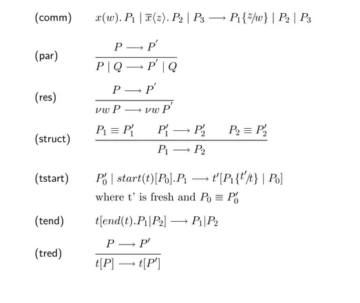
The reduction relation −→ is the smallest over processes obtained by applying the axioms and rules in Table 1.
The first four rules are the standard π-calculus ones. Here we report some observations on comm, for the other ones see ([9, 15]). The rule (comm) describes the communication among two parallel processes. Since we cannot transform t[π.P ] into π.t[P ], the communication is possible only between two standard processes both outside or both inside the transaction. Indeed, if we supposed t[π.P ] ≡ π.t[P ], it would be possible to make a communication between the internal processes of the transaction and processes outside or among two different transactions (the atomicity and isolation properties fail).
The axiom (tstart) describes the start of a transaction. The process P1
in-dicates some of the actions involved. We introduce the process P0inside the
square brackets to specify the elements to block, since necessary for the ex-ecution of the transaction. In this way, after the starting of the transaction,
(comm) x(w). P1| xhzi. P2| P3−→ P1{z/w} | P2| P3 (par) P −→ P 0 P | Q −→ P0 | Q (res) P −→ P 0 νw P −→ νw P0 (struct) P1 ≡ P 0 1 P 0 1 −→ P 0 2 P2 ≡ P20 P1 −→ P2 (tstart) P00 | start(t)[P0].P1 −→ t0[P1{t 0 /t} | P0]
where t’ is fresh and P0≡ P00
(tend) t[end(t).P1|P2] −→ P1|P2
(tred) P −→ P
0
t[P ] −→ t[P0]
Table 1: Axioms and rules for the reduction relation for π-calculus with biological transactions.
they cannot be consumed by other external processes. When an external process P00 structural congruent to the process P0 is found, the transaction
may start and P00 is put inside it. Finally, the result is a transaction of name t’ (t’ must be a fresh name) described by the internal process P1{t
0
/t}|P00. The axiom (tend) describes the successful end of the transaction t. As result of the transaction, the process P1 (after it) and the other internal processes
in parallel are given. The last rule expresses how the transaction is reduced: the reductions of the transaction t[P ] is described by the reductions of the internal process P.
We do not need an abort action as we assume that the internal process of a transaction is well-defined (i.e. it reduces to a parallel composition of processes among which the end(t).P is presented and so the transaction ends successfully).
3.3 Atomicity and Serializability
Some results are reported showing that biological transactions satisfy the desired atomicity (limited to simple biological systems) and serializability properties. Indeed, they are general criteria for proving the correctness of the transactions. We follow the same approach proposed in [2] and adapt it to our case. First of all, we add labels to each transaction to show what kind of action it represents. The labels (ranged over by l, l0, ....) are defined by the set L = {comm(x), t : comm(x), t : start, t : end} where x ∈ N and t ∈ T . The first label represents a communication between two processes outside a transaction along the channel x, while the others refer to actions involving a transaction of name t. They are the communication between two processes along x inside the transaction t, the start and the end of t. The reduction relation defined in 3.2 may be extended by considering these labels in the obvious way. Two functions are introduced to show the transaction names in a given label and to denote the set of transactions (processes of the form t[P ]) in a process P, respectively. The former (from L to T ) is defined as tr(t : comm(x)) = tr(t : start) = tr(t : end) = t and tr(comm(x)) = ⊥ (the symbol ⊥ stays for undefined). The latter one (from processes to T ) is defined as actT (P ) = {t|t[P0] for some P0 is a subterm of P }. As follows
we use the notation P0 σ
−→ Pn to denote the sequence P0 l1
−→ P1 l2
−→ P2... −→ Pln n, where σ = l1...ln. The transaction sequence P −→ Pσ 0, with
actT (P ) = actT (P0) = ∅, is serialized iff li = t : comm(x) or li = t : start
implies li+1 = t : comm(x) or li+1 = t : end for i = 1, ...(n − 1). The
internal processes are supposed to be well-defined. At this point we claim the following results:
Lemma 1. If P −→ Pl1 0 l2
−→ P00, with tr(l1) 6= tr(l2) and l1 = comm(x)
then there exists P000 such that P −→ Pl2 000 l1
This lemma shows that two transactions involving any two actions (not in the same transaction) are permutable.
Proof. In the proof we consider the following result deriving from the reduc-tion rules:
Lemma 2. Given P −→ Pl 0, we have that
• if l = comm(x) then P ≡ x(z).P1|xhwi.P2|Q and P0≡ P1{w/z}|P2|Q
• if l = t : comm(x) then P ≡ t[x(z).P1|xhwi.P2|Q]|R and
P ≡ t[P1{w/z}|P2|Q]|R
• if l = t : start then P ≡ start(t0)[P0].P1|Q and P0 ≡ t0[P0|P1{t 0
/t}]|Q • if l = t : end then P ≡ t[end(t).P0|P1]|Q and P0≡ P0|P1|Q
Considering lemma 3.3, since l1 = t : comm(x), we have that a process of
kind t[P1] is a sub-term of P , t[P10] is a sub-term of P0 and t[P1] l1
−→ t[P0 1], for
opportune P1and P10. Secondly, since tr(l1) 6= tr(l2) the label l2 refers either
to a transaction different from t or to a transition not involving transactions. Besides, there exists a process P2 and a process P20 such that P2 −→ Pl2 20 and
P2 is a sub-term of P0 and of P . From the previous observations, it is
inferred that P ≡ t[P1]|P2, P0 ≡ t[P10]|P2 and P00 ≡ t[P10]|P20.
Further-more, P ≡ P2|t[P1] (by applying structural congruence). If the rule par is
first applied considering P2 l2
−→ P20, we obtain P −→ Pl2 20|t[P1] and finally
by considering t[P1] l1
−→ t[P0
1], we derive the following transition sequence:
P −→ Pl1 20|t[P1] l1
−→ P20|t[P10] ≡ t[P10]|P20 ≡ P00. The process P20|t[P1] is the
process P000 we are looking for.
Theorem 1 (Seralizability). If P −→ Pσ1 0 with actT (P ) = actT (P0) = ∅, then there exists a permutation σ2 of σ1 such that P
σ2
−→ P0 is serialized. Proof. Let σ1 be l1l2....ln with n ≥ 1. We have to show that there exists
a permutation σ2 = l01l02l03....ln0 of σ1 such that P σ2
−→ P0 is serialized. The proof is by induction on the length of σ1. Some preliminary definitions and
results are given.
The length of σ is defined as: • length(σ) = 1 if σ = l
• length(σ) = n if σ = l1l2....ln
Besides, the following two assertions are derived from the reduction rules: Assertion 1 If P −→ Pl 0 with actT(P ) = {t} and l = t : end then
Assertion 2 If P −→ Pl 0with act
T(P ) = ∅ and tr(l) = ⊥ then actT(P0) = ∅
Given n = length(σ1), we consider the two cases:
1. If n = 1, the only possibility is that σ1 = l1 and tr(l1) = ⊥ and it is
obviously serialized.
2. If n > 1, we have two possibilities:
• tr(li) = ⊥ for ∀i ∈ [1, ..., n], it is obviously serialized.
• There exist (at least two) labels in σ1 for which tr(l) = t. Let be lk(with k < (n−1)) the first transition label with tr(lk) 6= ⊥. We
have that li0 = li for i = 1, ..., k. As actT (P0) = ∅ (from assertion
2 ), it follows that actT (Pi) = ∅ for i < k. From this, we can
deduce that lk = t : start. Consider the label l(k+1). There are
three different cases:
(a) if l(k+1) = t : end then l0(k+1) = l(k+1). In the case (k + 1) = n we conclude σ2 = l1l2...lkl(k+1). Otherwise, since
Act(k+1)= ∅ from the assertion 1, for the inductive
assump-tion on P(k+1) σ10
−→ Pnthere exists σ02for which the transition sequence is serialized. We conclude that σ2 = l1l2...l(k+1)σ02.
(b) If (k+1) = t : comm(x) then l0(k+1) = l(k+1). Then we need
to consider the following elements until l = t : end is found. According to the kind of labels, at each step we proceed as in (b) or (c). When l = t : end is found we apply the inductive assumption on the rest of the sequence as seen in (a). (c) If tr(l(k+1)) 6= t, we consider the first s such that tr(l(k+s)) =
t (with s > 1). At this point the lemma 1 is applied (s − 1) times and we finally obtain the sequence P(k+1)
l(k+s)
−→ P(k+2)0 l(k+1)−→ ...P(k+s) σ
0 1
−→ P0. The transaction labeled l (k+s)
moves at the (k + 1) position and l(k+1)0 = l(k+s). If l(k+s)=
t : end then Act(P(k+s)0 ) = ∅ (from assertion 1 ) and we may applied the inductive assumption on P(k+s) σ
0 1
−→ P0 as seen
for (a). Otherwise, we consider the next element and proceed as seen until t : end is found.
Corollary 1. If P −→ Pσ1 0 and actT (P ) = {t} then there exists σ
2 and σ3,
with σ2σ3 a permutation of σ1, such that for each l ∈ σ2 tr(l) = {t} and
Proof. It follows directly from the application of Lemma 3.3 to move all the transitions involving t to the first positions. We can say that σ2 is
given by the sequence of labels so found (tr(l) = t for each of them for construction) and σ3 is given by the rest of the labels. Besides, σ2σ3 is
clearly a permutation of σ1.
Given a sequence of transitions involving one or more transactions, it is so possible to obtain a permutated sequence that is serialized, i.e. in which the transactions may be executed one after the other. As for the corollary, it says that if in a sequence of transitions some refer to a transaction t, it is possible to permutate the transitions such that all the actions involving t are not interleaved by other actions.
Concerning atomicity, we first need to define simple biological systems, for which the property is guaranteed. These are systems where it is not possible to have processes that could execute infinitely in parallel with a transaction. If more general systems were considered, it could happen that a transaction starts but does not commit in a finite number of steps as its transitions are interleaved by transitions involving external processes. For instance, if the transitions S1
l1
−→ S2 and S2 l2
−→ S1 are considered, then it could happen that the following sequence is obtained: P0|S0 l1
−→ P0|S 2 l2 −→ P0|S1 l1 −→ P0|S
2... and so on infinitely. The transaction has started, but does
not complete, at least in a finite time. We consider the following theorem: Theorem 2 (Atomicity). Let be P = start(t)[P0].P1|P00, with P00 structural
congruent to P0 and P00|P1{t 0
/t} well defined. If P −→ Pl 0 with l = (t0: start)
and P0 = t0[P00|P1{t0/t}], then always P0|S −→ Pσ 00|S0 for any(finite length)
sequence σ, where P0|S is a simple biological system and P00 indicates the final process of the transaction.
Proof. Given the process P0 = t0[P00|P1{t 0
/t}] as the internal process is well-defined from the hypothesis, there exists a sequence of n transitions σ0 =
l01l02...l0n such that P0−→ Pσ0 00 where P00 is the final result of the transaction.
As the system S0 is a simple biological system, it always reduce to a final process in a finite number of steps and we indicate with σ1 any possible finite
length label sequence. Consider P0|S. All possible reductions are obtained from the possible transitions of the two sub-processes and by applying the rule par. Consequently, σ is defined by considering the labels in σ0 and σ1
according to the possible order of action selection. From this observation, we conclude that the sequence σ has finite length.
If we wanted to extend the theorem to more general models, it would be necessary to add a new action to abort the transactions after some time and give an opportune compensation to rollback to the initial situation.
4
Application of transactions to model reactions
In this section, some explicative examples about the application of trans-actions to model biological retrans-actions are presented. These examples are about:
• three-reactant reactions
• two-modifier one-reactant reactions • one reaction from the citric acid cycle
Finally, some observations about the introduction of the non-deterministic choice are reported.
4.1 Examples about reactions
4.1.1 Three-reactant reaction R1+ R2+ R3 → P
The reaction R1+ R2 + R3 → P represents a generic reaction with three
reactants and one product. In section 2.1, a possible way to translate the reaction using the standard π-calculus has been shown and discussed. Here we describe how to model it by using biological transactions. The reaction is represented by using transactions as:
T123 = start(t)[P2|P3].P1|P2|P3
P1 = x12hi. x123hi. end(t).PP r
P2 = x12(). nil P3 = x123(). nil
where PP rrepresents the process describing the product P . The system
S = S0| T123 (where S0 indicate a process different from P) may be reduced as:
T123| S0 −→ t0[x12hi. x123hi. end(t0).PP r | x12(). nil | x123(). nil] | S0
−→ t0[x123hi. end(t0).PP r| nil | x123(). nil] | S0
−→ t0[end(t0).PP r | nil | nil] | S0
−→ PP r | nil | nil | S0≡ PP r| S0
The term with the start of the transaction describes initially the activity of only one reactant (R1) and the actions of the other two reactants R2 and
R3 are described by (initially) external processes. Only after the transaction
t0has started, all the processes involved in it move inside t0. This permits the composition of the model from the processes describing each species, as in π-calculus. Finally, the approach proposed is easily extendible to reactions with more reactants and products.
4.1.2 Reaction of kind R + E1+ E2→ P + E1+ E2
This reaction represents an enzymatic reaction with one reactant R and two enzymes E1and E2. This kind of reaction is generally used as an abstraction
of a sequence of elementary reactions. Transactions are useful when we do not know how to decompose the reaction in meaningful elementary steps and as a consequence would be desirable to represent the whole reaction as an atomic one. Following the approach proposed previously, the reaction may be modeled as:
TRE1E2 = start(t)[P
0
2|P30].P1| P20 | P30
where P1 is defined as in the previous example, P20 = x12().P20 and P30 =
x123().P30.
A possible reduction of the system S = S0|TRE1E2 is given by:
TRE1E2 | S
0 −→ t0[x
12hi. x123hi. end(t0).PP r| x12(). P20 | x123(). P30] | S0
−→ t0[x123hi. end(t0).PP r| P20 | x123(). P30] | S0 −→ t0[end(t0).PP r| P20 | P30] | S0 −→ PP r| P20 | P 0 3 | S 0
4.1.3 One example from citric acid cycle
The citric acid cycle (also known as the Krebs cycle) is part of a metabolic pathway involved in the chemical conversion of carbohydrates, fats and pro-teins into carbon dioxide and water to generate a form of usable energy. The model (taken from the KEGG metabolic pathway database, [5]) consists of a series of chemical reactions of central importance in all living cells that involves a lot of proteins, molecules and enzymes. Here we focus only on the first reaction of the cycle, where the Acetyl-CoA (the activated acetic acid) reacts with oxaloacetate (the four carbon carboxylic acid) to form citrate and CoA. The reaction is catalyzed by the enzyme citrate-synthase (CS). The reaction as the following form:
Acetyl CoA + Oxoloacitate + CS → CoA + Citrate + CS The reaction is represented by using transactions as:
Tf irst = start(t)[Ox|CitSynt](AcCoA)|Ox|CitSynt
AcCoA = x12hi. x123hi. end(t).(CoA|Citrate)
Ox = x12(). nil
where CoA and Citrate represent the processes describing the two prod-ucts. Supposing that the initial system is of the form S = Tf irst|S0, one of
the possible reduction is:
Tf irst | S0 −→ t0[x12hi. x123hi. end(t0).(CoA|Citrate) | x12(). nil |
x123(). CitSynt] | S0
−→ t0[x123hi. end(t0).(CoA|Citrate) | nil | x123(). CitSynt] | S0
−→ t0[end(t0).(CoA|Citrate) | nil | CitSynt] | S0 −→ (CoA|Citrate) | nil | CitSynt | S0
where (CoA|Citrate) | nil | CitSynt | S0≡ CoA|Citrate|CitSynt | S0.
4.2 Non-deterministic choice
In describing biological models, it often happens that a biological entity (as a gene or a protein) is involved in more than one reaction and only one of the possible reaction may be selected. This situation is modeled in π-calculus by using the operator choice +. The process P + Q (to be added to the process syntax definition) describes a process that behaves either as P or as Q. For instance, if the system is composed of three proteins A, B, C, involved in the reactions r1 : A + B → C and r2 : A + C → C, the protein
A may be consumed in both the reactions. The system may be described by S = PA| PB| PC, with PA= xABhi.PC+ xAChi. nil, PB = xAB(). nil and
PC = xAC().PC.
If a new reaction r3 : A + E + F → D is added, a transaction may
be defined to model it, as seen in 4. We indicate with TAEF the process to
describe the transaction. The specification of the system composed of only one reactant for type and described by the three reactions r1, r2 and r3 is:
S = (TAEF + PA)|PB|PC|PE|PF
where TAEF = (start(t)[PE|PF]. PA0) with PA0 = xAEhi. xAEFhi. end(t). PD,
PE = xAE(). nil, PF = xAEF(). nil. PB and PC are the ones defined
previ-ously.
Respect to the definition of the calculus presented in 3, we must add the process P + Q to the syntax definition and modify the rule comm (in the usual way), the axiom tstart and the axiom tend. The new rules are:
(tstartChoice) (P1+ Q1)|...|(Pn+ Qn)|S|start(t)[P10|...|P 0 n].P0+ Q0 −→ S | t0[P0{t 0 /t}|P1|...|Pn]
where t0 fresh and Pi ≡ Pi0 and for i = 1, .., n
(tEndChoice) t[end(t).P1+ Q1|P2] −→ P1|P2
5
Discussion and conclusions
This work presents an extension of the synchronous π-calculus with trans-actions to model multiple-reactant multiple-product retrans-actions. These reac-tions, rare in nature, are quite frequent in biological models. Some problems arise when we model them by using a sequence of pair-wise communication in the standard π-calculus, as it cannot be represented atomically. A possi-bility to override this problem is to consider transactions, since they allow to represent a sequence of elementary actions as an atomic one. The trans-actions considered here have simple features suitable for our purposes. They are called biological transactions to distinguish them from the more complex ones used in web-service and database fields. An extended calculus has been defined and then some examples about its application have been shown and discussed.
In this work, we focus only on qualitative models. In the future we aim to define a stochastic version of this extended calculus. This would make pos-sible to model complex reactions as atomic actions also in the quantitative case. The approach to follow is the one proposed in [11] for the standard stochastic π-calculus. The idea is to enrich each prefix with a rate, that represents the parameter of an exponential distribution that characterizes the stochastic behavior of the activity corresponding to the associate prefix. In addition, the semantics should be modified to consider the quantitative information. As in [11], the reference algorithm is the one proposed in Gille-spie [4], but a generalized version should be considered, as in transactions more than two processes are involved. Concerning the rule par, we should refer to the possible subcases, that correspond to the possible actions. In addition to the functions to count the number of input and output processes on the channel x, we would need to define a function to count the number of processes congruent to a given one. A critical point is how to count the input and output on a channel x when a communication is enabled inside a transaction. A possible idea is to consider all the inputs and the out-puts enabled in the system and not only the ones inside the transaction. All these ideas will be better developed and formalized in a future work. Another possible extension of this paper is to introduce opportune abort actions and compensation mechanisms. This would permit to extend the atomicity property to more general systems.
References
[1] L. Bocchi, C. Laneve, and G. Zavattaro. A calculus for long-running transactions. In Proc. of FMOODS’03, volume 2884 of Lecture Notes in Computer Science. Springer-Verlag, 2003.
[2] N. Busi and G. Zavattaro. On the serializability of transactions in javaspaces. In Proc. of CONCOORD’01, volume 54 of Lecture Notes in Computer Science. Springer-Verlag, 2001.
[3] M. Butler, T. Hoare, and C. Ferreira. A trace semantics for long-running transactions. In Proc. of 25 year of CSP, volume 3525 of Lecture Notes in Computer Science. Springer-Verlag, 2005.
[4] D.T. Gillespie. Exact stochastic simulation of coupled chemical reac-tions. Journal of Physical Chemistry, 81(25):2340–2361, 1977.
[5] M. Kanehisa and S. Goto. KEGG: Kyoto Encyclopedia of Genes and Genomes. Nucleic Acids Res., (28):27–30, 2000.
[6] C. Kuttler, J Niehren, and R. Blossey. Gene regulation in the π-calculus: simulating cooperativity at the lambda switch. In Second international workshop on concurrent models in molecular biology (BioConcur 2004), 2004.
[7] C. Laneve and G. Zavattaro. Foundations of web transactions. In Proc. of FOSSACS 2005, volume 3441 of Lecture Notes in Computer Science. Springer-Verlag, 2005.
[8] P. Lecca, C. Priami, P. Quaglia, B. Rossi, C. Laudanna, and G. Costantin. Language modeling and simulation of autoreactive lym-phocytes recruitment in inflamed brain vessels. SIMULATION: Trans-actions of The Society for Modeling and Simulation International., 80, 2004.
[9] R. Milner. Communicating and mobile systems: the π-calculus. Cam-bridge University Press, 1999.
[10] C. Priami and P. Quaglia. Beta binders for biological interactions. In Computational Methods in Systems Biology ’04 (CMSB04), 2004. [11] C. Priami, A. Regev, W. Silverman, and E. Shapiro. Application of
a stochastic name-passing calculus to representation and simulation of molecular processes. Information Processing Letters, 80(1):25–31, 2001. [12] A. Regev. Representation and simulation of molecular pathways in the stochastic π-calculus. In Proceedings of the 2nd workshop on Compu-tation of Biochemical Pathways and Genetic Networks, 2001.
[13] A. Regev, E. M. Panina, W. Silverman, L. Cardelli, and E. Shapiro. Bioambients: An abstraction for biological compartments. Theoretical Computer Science, 325(1):141–167, September 2004.
[14] A. Regev, W. Silverman, and E. Shapiro. Representation and simula-tion of biochemical processes using the π-calculus process algebra. In Proceedings of the Pacific Symposium of Biocomputing 2001, volume 6, pages 459–470, 2001.
[15] D. Sangiorgi and D. Walker. The π-calculus: a Theory of Mobile Pro-cesses. Cambridge University Press, 2001.
[16] V.Danos and J.Krivine. Formal molecular biology done in CCS-R. In BioConcur ’03, Workshop on Concurrent Models in MolecularBiology, 2003.