Solutions to common issues in widefield microscopy: vignetting, mosaicing and depth of focus

ARCES - Advanced Research Center on Electronic Systems for Information and Communication Technologies “Ercole De Castro”

European Doctorate in Information Technology Cycle XXV

09/G2 - Bioengineering; ING-INF/06

SOLUTIONS TO COMMON ISSUES IN WIDEFIELD

MICROSCOPY: VIGNETTING, MOSAICING

AND DEPTH OF FOCUS

Filippo Piccinini

Coordinator Prof. Claudio Fiegna

Tutor

Prof. Alessandro Bevilacqua

Co-Tutor

Prof. Mauro Ursino

PhD course: January 1, 2010 - December 31, 2012 Final exam: April 19, 2013

Si chiude una porta, si apre un portone.

Prof. Emanuele Trucco, University of Dundee, Scotland, email: manueltrucco@computing.dundee.ac.uk

Prof. Walter G. Kropatsch, Vienna University of Technology, Austria, email: krw@prip.tuwien.ac.at

IMAGE PROCESSING

FLUORESCENCE MICROSCOPY

BRIGHT FIELD

PHASE CONTRAST

BIOMEDICAL IMAGING

In this thesis we have studied and developed solutions to common issues re-garding widefield microscopes, facing the common problem of the intensity inhomogeneity of an image and dealing with two strong limitations: the impos-sibility of acquiring either high detailed images representative of whole samples or deep 3D objects.

First, we cope with the problem of the non-uniform distribution of the light signal inside a single image, named vignetting , making the objects of the image hardly comparable. In particular we proposed, for both light and flu-orescent microscopy, non-parametric multi-image based methods, where the vignetting function is estimated directly from the sample without requiring any prior information. After getting flat-field corrected images, we studied how to fix the problem related to the limitation of the field of view of the camera, so to be able to acquire large areas at high magnification. To this purpose, we developed mosaicing techniques capable to work on-line. Start-ing from a set of overlappStart-ing images manually acquired, we validated a fast registration approach to accurately stitch together the images previously flat-field corrected. Finally, we worked to virtually extend the flat-field of view of the camera in the third dimension (i.e., the z -dimension), with the purpose of reconstructing a single image completely in focus, stemming from objects having a relevant depth or being displaced in different focus planes. To pursue this goal, a stack of images is typically acquired by scanning the objects in z. Several methods have been proposed in literature to estimate the in-focus re-gions in each image of the stack to reconstruct one image completely in focus. After studying the existing approaches for extending the depth of focus of the microscope, we proposed a general method that does not require any prior information. In order to compare the outcome of existing methods, different standard metrics (Universal Quality Index, Signal to Noise Ratio and Mean

cases to compare different methods, where a reference ground truth is not at one’s disposal. First, we validated a metric able to rank the methods as the Universal Quality Index does, but without needing any reference ground truth. Second, we proved that the approach we developed performs better in both synthetic and real cases.

The thesis contains data and methods that we have partly published in 3 scientific journals and 6 international conference proceedings. All the source codes and related material are achievable upon request.

In questa tesi abbiamo studiato e sviluppato soluzioni a questioni comuni in materia di microscopia a campo largo. In particolare abbiamo affrontato il problema della non omogeneit´a dell’intensit´a delle immagini acquisite e due forti limitazioni: l’impossibilit´a di acquisire immagini ad alto dettaglio rappre-sentative o dell’intero campione o di oggetti 3D con spessore non trascurabile. Per prima cosa abbiamo studiato le caratteristiche del problema denominato vignettatura, relativo alla distribuzione non uniforme del segnale di luce all’interno di ogni singola immagine che rende gli oggetti presenti difficilmente paragonabili. In particolare abbiamo proposto, sia per la microscopia a luce sia per la microscopia a fluorescenza, metodi non parametrici dove la fun-zione di vignettatura ´e stimata utilizzando un insieme di immagini acquisite direttamente dal campione, senza richiedere alcuna informazione aggiuntiva. Dopo aver sviluppato metodi per ottenere immagini con distribuzione uniforme di intensit´a, abbiamo studiato come risolvere il problema legato alla limitata dimensione del campo di vista della telecamera, al fine di essere in grado di ac-quisire una singola immagine ad alto ingrandimento rappresentativa dell’intera area del campione osservato. A questo scopo abbiamo sviluppato tecniche di mosaicatura in grado di operare on-line con l’acquisizione delle immagini. Partendo da una serie di immagini acquisite manualmente, avendo cura che ci fosse sempre una certa percentuale di sovrapposizione tra due immagini seguenti, abbiamo validato un approccio di registrazione in grado di creare ve-locemente un mosaico allineando accuratamente le singole immagini acquisite, precedentemente corrette dall’effetto di vignettatura. Infine, abbiamo studi-ato come estendere virtualmente il campo di vista della telecamera lungo la terza dimensione (la dimensione z ), con lo scopo di poter ottenere singole im-magini completamente a fuoco o di oggetti aventi uno spessore rilevante o di un insieme di oggetti posizionati su differenti piani di messa a fuoco.

Gen-letteratura per stimare prima le regioni a fuoco in ogni singola immagine e a se-guito per ricostruire l’immagine completamente a fuoco sfruttando le regioni a fuoco precedentemente identificate. Dopo aver studiato i vari approcci esistenti per estendere la profondit´a di messa a fuoco del microscopio, abbiamo proposto un metodo generale che non richiede alcuna informazione a priori. Per confrontare i risultati dei diversi metodi, in letteratura sono tipicamente usate diverse metriche comuni (indice di qualit´a universale, rapporto segnale rumore ed errore quadratico medio) sfruttando immagini sintetiche dotate di verit´a di riferimento. Tuttavia nessuna metrica in grado di confrontare diversi metodi analizzando i risultati ottenuti usando immagini reali dove non ´e pre-sente l’immagine di verit´a. In primo luogo abbiamo validato una metrica in grado di classificare i diversi metodi in accordo all’indice di qualit´a universale ma senza bisogno di alcuna verit´a di riferimento. Poi, sfruttando la metrica validata e sequenze di immagini sintetiche, abbiamo dimostrato che il metodo che abbiamo sviluppato risulta essere il migliore tra tutti quelli testati per estendere la profondit´a di messa a fuoco.

Questa tesi contiene dati e metodi in parte gi´a pubblicati in 3 riviste scientifiche e 6 atti di conferenze internazionali. Tutto il materiale citato, compreso il codice sorgente dell’implementazione dei metodi, ´e fornito su richiesta.

Abstract (English version) xi

Abstract (Italian version) xiii

Contents xv

1 Introduction and thesis overview 1

2 Vignetting in light microscopy 9

2.1 Introduction . . . 10

2.2 State of the art . . . 14

2.3 Methods . . . 18

2.3.1 Background segmentation . . . 21

2.3.2 Dense background reconstruction . . . 22

2.4 Materials and tools . . . 23

2.5 Experimental results . . . 24

2.5.1 Quality of the background segmentation . . . 25

2.5.2 Vignetting function of image number and confluence . . 28

2.5.3 Comparison of shapes of different vignetting functions . . 30

2.5.4 Flat-field correction on single images . . . 32

2.5.5 Flat-field correction on mosaics . . . 35

2.6 Conclusion and future work . . . 41

2.6.1 Conclusion . . . 41

2.6.2 Future work . . . 43

2.7 Acknowledgments . . . 44

2.8 Copyright permission . . . 44

3 Vignetting in fluorescence microscopy 47 3.1 Introduction . . . 48

3.4 Method based on linear correction . . . 58

3.4.1 Background modelling . . . 58

3.4.2 Vignetting estimation . . . 59

3.4.3 Linear flat-field correction . . . 61

3.5 Method based on non-linear correction . . . 62

3.5.1 Photobleaching modelling . . . 64

3.5.2 Vignetting functions estimation . . . 65

3.5.3 Non-linear flat-field correction . . . 66

3.6 Experimental results . . . 67

3.6.1 Flatness of the foreground signal . . . 68

3.6.2 Flatness of the whole images . . . 71

3.7 Conclusion and future work . . . 77

3.7.1 Conclusion . . . 77

3.7.2 Future work . . . 79

3.8 Acknowledgments . . . 80

4 Mosaicing 81 4.1 Introduction . . . 82

4.2 State of the art . . . 85

4.3 Methods . . . 91

4.3.1 Pre-processing . . . 91

4.3.2 Feature Detection . . . 93

4.3.3 Feature Matching . . . 95

4.3.4 Warping Model Estimation . . . 97

4.3.5 Image Warping and Stitching . . . 100

4.4 Materials . . . 102 4.5 Metrics . . . 105 4.6 Experimental results . . . 108 4.6.1 Flat-field correction . . . 108 4.6.2 F2M registration . . . 110 4.6.3 Warping models . . . 111

4.6.4 Results using the histological specimen . . . 114

4.6.5 Histological sample versus cell culture . . . 117

4.6.6 Computational performance . . . 118

4.7 Conclusion and future work . . . 119

5 Depth of focus 125

5.1 Introduction . . . 126

5.2 State of the art . . . 129

5.3 Methods . . . 131

5.4 Quality metrics . . . 134

5.5 Materials . . . 136

5.6 Experimental results . . . 139

5.6.1 Experiments with the synthetic stacks . . . 140

5.6.2 Analysis of metrics for real stacks . . . 141

5.6.3 Experiments with real stacks . . . 144

5.7 Conclusion and future work . . . 145

5.7.1 Conclusion . . . 145 5.7.2 Future work . . . 147 5.8 Acknowledgments . . . 147 5.9 Copyright permission . . . 148 6 Conclusion 149 Appendix 153 Phase correlation . . . 153 RANSAC . . . 156 List of figures 159 List of tables 161 Bibliography 163 Personal publications 183 Thanks 185

Introduction and thesis

overview

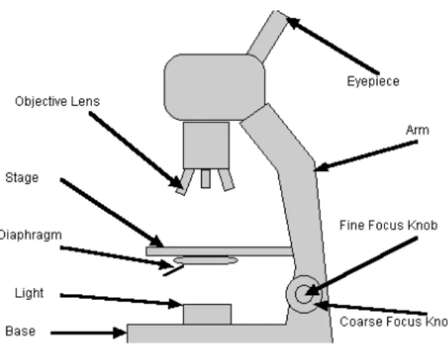
Fig. 1.1: Widefield microscope. Schematic representation of the principal compo-nents

Nowadays, the extent of human knowledge is widening by managing from macro to nano. In the infinite big, we are able to remotely drive a robot to collect materials on Mars. In the infinite small, we manage the human DNA to prevent severe illness. In particular, these great goals of the humanity are brought from a general improvement on every contributing science. And there is a common fundamental line in the improvement of every single science: the possibility to perform measurements. This is the fundamental key point of the

MICROSCOPES ELECTRON OPTICAL CONFOCAL WIDEFIELD LIGHT FLUORESCENCE PHASE-CONTRAST BRIGHTFIELD ...

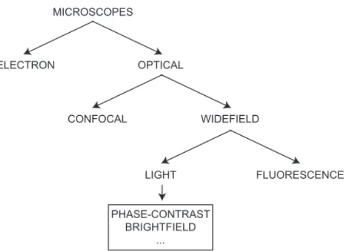
Fig. 1.2: Microscoscopes taxonomy. Simplified schematic tree diagram of common microscope types

general knowledge improvement. Measuring a phenomenon, we become able to study, and often also to control and modify that phenomenon. In particular, in this thesis we focus our attention on one limit of the human knowledge, the infinite small, where there is a main instrument of measurement: the microscope (Fig. 1.1) [1].

Lens systems and microscopes are used in science from the sixteenth century, always increasing their magnification capabilities [2]. Now, in the twenty-first century, we are in the middle of two Ages of microscopes: the Age of micro and the Age of nano. The magnification factor has become so high that we can look into a single micro cell and study nano particles [3]. Furthermore, so many variants of microscopes have been realized that is also difficult to define a proper taxonomy [4]. In Fig. 1.2 a simplified schematic tree diagram is proposed, organized in the upper part accordingly to the technology, then to the imaging techniques.

As expected, there is not a general microscopy technique suitable for all pur-poses [5]. Before choosing the microscope fulfilling our requirements, we need to define our goal: what do we want to see. For instance, looking at a high mag-nification the cell shape does not help for defining an animal species (Fig. 1.3). Accordingly, the wide range of different microscopes available is the answer to visualize different particular characteristics of the substances. Neverthe-less, despite the wide availability of many different microscopes and the new technology continuously improving the performance of devices, there are still

Fig. 1.3: Microscope and measure. The choice of the measurement instrument is always tight to what we want to measure. Cartoon by Gary Larson.

problems and limitations that have to be faced [6].

In this thesis, we focus our attention on optical widefield microscopy, the most present in biological laboratories. This class of microscopes can be subdivided into more groups according to the illumination source used to visualize the substance (Fig. 1.4), typically rays of given wavelength in the human visible spectrum (Light Microscopy [7], 700 ηm - 400 ηm) or, more extensively, from the infrared to the ultra violet (Fluorescence Microscopy [8], 1000 ηm - 1 ηm). These microscopes are principally used in brightfield and phase-contrast [9] to visualize the morphology of micrometric cells and, in fluorescence, to high-light nanometric particles or cell structures. As far as the general widefield microscopy is concerned, limitations are often related to the area’s extension achievable in one single image at the desired resolution and to the visualization of deep objects, characterized by a relevant z -dimension (e.g., large 3D mul-ticellular aggregates). Moreover, there are problems arising from the uneven distribution of the signal in the field of view. Furthermore, specifically in flu-orescence microscopy, problems such as photo-bleaching and quenching effect

Fig. 1.4: Light spectrum. The Human visible light is between 700 ηm - 400 ηm.

From Wikipedia: electromagnetic spectrum.

limit the concept to consider a microscope an instrument of measurement. The lofty objective of this thesis and of all the methods generally proposed in liter-ature to fix problems or relax limitations, is to improve technology, techniques and knowledge in order to make the microscope more and more an accurate quantity measuring system [10].

This thesis deals with three main common issues of the widefield microscopy: • correction for the uneven distribution of the signal

• acquisition of an image of a large area at a high magnification • visualization of deep objects

The keywords related to these issues are respectively: vignetting, mosaicing and depth of focus.

VIGNETTING: the uneven fall-off of the image intensity (Fig. 2.1). This problem affects all the images acquired with a widefield microscope, making the distribution of the signal non homogeneous. If no correction is accomplished, the images are almost useless for quantitative analyses. Often, to correct for

vignetting, reference images are acquired in advance to characterize the signal distribution and use the function estimated as a normalization factor. Never-theless, several reasons make this solution infeasible. The vignetting problem is analyzed in both light (brightfield and phase-contrast) and fluorescence mi-croscopy and multi-image based methods to estimate the vignetting function from the sample itself are proposed.

MOSAICING: the stitching of a set of images aiming at virtually extending the limited field of view of the camera (Fig. 4.1). The final result is a mosaic having at least the same pixel resolution of the source images and a large final represented area. Mosaicing is a very common technique, used in many applications such as panoramic photography, satellite imaging and biological applications. Accordingly, many methods are proposed in literature to obtain accurate mosaics in microscopy. Several of them relied on priors, like the shifts between the images. A non-parametric method is proposed to stitch together images manually acquired with a standard widefield microscope, even though not coupled with a motorized x -y stage.

DEPTH OF FOCUS: key parameter of optical system, sometimes also called depth of field (Fig. 5.1). In the data sheet of the lens, it is normally expressed in µm. It represents the distance between focal planes in the z -dimension, where objects keep sharp or in focus. An object is considered in focus when it is particularly sharp, clear and, in general, good-looking. This parameter is a strong limitation for the system, because it makes the acquisition of sharp images of deep objects infeasible. Several methods are proposed in literature to overcome this limit, but it is particularly difficult to compare the results due to the lack of the “ground truth”, that is a gold standard assumed to be the “truth”. In particular, a metric based on the Universal Quality Index that does not require the ground truth is validated. Then, the methods at the state of the art are compared meanwhile proposing a new solution that does not require prior information on the images acquired nor heavy computational burden.

This thesis is organized as follows:

Chapter 2 discusses the vignetting problem in all the details regarding light microscopy. After an introduction on causes and effects, the state-of-the-art methods are presented and compared. Then, a multi-image based method to

estimate the vignetting function from the sample itself is proposed, overcoming the other approaches considered.

In Chapter 3 the vignetting is analyzed in fluorescence microscopy. Usually, problems like photobleaching, quenching and background behaviour make the methods proposed in light microscopy ineffective. After an exhaustive analy-sis of the available solutions, two different methods to correct the images by the vignetting effect are proposed. In the first one, the vignetting function is estimated from a large set of images acquired in advance. In the second one, an ensemble of vignetting functions (instead of a single one) is estimated (reg-istering a set of overlapping images) and a non linear correction is proposed instead of the linear one commonly used.

Chapter 4 presents the mosaicing technique as a solution to easily extend the field of view of digital cameras coupled with microscopes. In particular, although the images are acquired with a microscope not coupled with a motor-ized x -y stage, the proposed general purpose registration approach works at subpixel, yielding highly accurate mosaics. The focus of this work it is not nec-essarily the advancing of the state of the art. Rather, it represents a functional stage for testing the different vignetting correction approaches. Nevertheless, at the same time a solution for building mosaics on-line using non-automated microscopes is proposed.

Chapter 5 is related to the depth-of-focus parameter. It is presented as a strong constraint of the microscopes for a certain type of biological analyses. A pretty fast method to extend the depth of focus is proposed. Furthermore, a new metric is proposed to compare the state-of-the-art methods without requiring the ground truth, typically not at one’s disposal.

Concluding remarks and hints for possible future work are reported and dis-cussed in Chapter 6.

The work developed in this thesis has been carried out with the:

• Computer Vision Group (CVG), II Faculty of Engineering, University of Bologna, Bologna, Italy. Director: Dr. Alessandro Bevilacqua

• Osteoarticular Regeneration Laboratory, Rizzoli Orthopaedic Institute (IOR), Bologna, Italy. Director: Dr. Enrico Lucarelli

• Laboratory of Biosciences, Istituto Romagnolo per lo Studio e la cura dei Tumori (IRCCS-IRST), Meldola (Forl´ı-Cesena), Italy. Director: Dr. Wai-ner Zoli

• Laboratory of Radiobiology, Istituto Romagnolo per lo Studio e la cura dei Tumori (IRCCS-IRST), Meldola (Forl´ı-Cesena), Italy. Director: Dr. An-na Tesei

• Light Microscopy and Screening Center, Eidgen¨ossische Technische Ho-chschule Z¨urich (ETHZ), Zurich, Switzerland. Responsible of Image Pro-cessing: Dr. Peter Horvath

the activities have been carried out in the following two projects:

• STAMINAL - characterization of STem cells through support for Auto-matic analysis of the MIcroscopic images in pre-cliNicAL therapy (par-tially granted by IRCCS-IRST)

• ADVANCE - Automatic non-invasive system based on high content anal-ysis to Detect and characterize VitAl meseNchymal stem Cells in a spatio-temporal contExt (partially granted by IOR)

In particular, I spent the first year for implementing and validating the mosaic-ing technique, then used to test the different vignettmosaic-ing correction approaches. In the following two years I have deeply explored the research field of vignetting correction in both light and fluorescent microscopy, yielding to innovate the state of the art. In the same time, I worked on the field of the extension of depth of focus for the visualization of deep objects, comparing the existing approaches and proposing a new effective solution. The developed methods and the obtained data have been partly published in 3 scientific journals and are presented in 6 international conference proceedings. All the source codes and related material are distributable upon request [11].

The 3-year PhD course in Information Technology was granted by the Ad-vanced Research Center on Electronic Systems (ARCES), University of Bologna, Italy.

Vignetting in light microscopy

Fig. 2.1: Vignetting effect. Inhomogeneous distribution of the image intensity.

- F. Piccinini, E. Lucarelli, A. Gherardi, A. Bevilacqua, Multi-image based method to correct vignetting effect in light microscopy images. Journal of Microscopy, 248(1): 6-22, 2012

- A. Bevilacqua, F. Piccinini, Is an empty field the best reference to correct vignetting in microscopy? 7th

International Workshop on Biosignal Interpretation (BSI), Como, Italy, July 2-4, 2012, pp. 267-270 - A. Bevilacqua, F. Piccinini, A. Gherardi, Vignetting correction by exploiting an optical microscopy image sequence. 33rd_{International Conference of the IEEE Engineering in Medicine and Biology Society (EMBS),}

Boston, USA, August 30-September 3, 2011, pp. 6166-6169

- A. Gherardi, A. Bevilacqua, F. Piccinini, Illumination field estimation through background detection in optical microscopy. 8th _{Annual IEEE Symposium on Computational Intelligence in Bioinformatics and}

2.1

Introduction

Nowadays, light microscopes coupled with digital cameras are part of the ordi-nary basic equipment of all biological laboratories, where most of the biological routine examinations regard cell cultures and histological samples. The accu-racy of the microscope system, meant as an ensemble of illumination source, condenser, filters, lens and camera sensors, has become particularly high even using cheap components, this making quantitative imaging examinations enter in daily routine [10]. Accordingly, great benefits in the biology research can derive from improvements in the image acquisition system as corrections of early errors still present [12].

Typically, the images acquired with light microscopes are characterized by a radial fall-off of brightness intensity from the principal point towards the image borders [13]. This undesirable property, intrinsic to optical systems, is known as vignetting and represents one of the most common early problems that af-fects digital imaging [14] and, in particular, subsequent processing stages such as segmentation [15] and object tracking [16]. The problem is far more empha-sized in quantitative imaging, where taking into account the vignetting effect is mandatory to achieve reliable intensity measurements [17] or to compare images achieved in subsequent times [18]. From a visual point of view, the problem becomes particularly evident in mosaicing, where several images are stitched together to fix the problem related to the narrowness of the field of view of the camera [19, 20]. In fact, the registered images are not corrected for vignetting effects, the seams in the stitching zones become clearly notable [21], misleading visual and automated analysis [22, 23].

The ideal condition to have a negligible vignetting effect is called K¨ohler illumi-nation [24, 25]. However, in real cases, many sources of vignetting contribute to find a fall-off of the image intensity [26]. In [27] are reported the main sources of vignetting classified according to the following four sources.

Natural vignetting, radial falloff due to geometric optics. Different regions of the image plane receive different irradiance. For simple lenses, these effects are sometimes modeled as a falloff of cos4_{(θ) [28, 29], where θ is the angle}

at which the light exits from the rear of the lens. Note that in all lenses, the distance from the exit pupil to the image plane changes when the focus distance is changed, so this component varies with focus distance. The cos4 _{law is only}

an approximation which often could not be enough to model properly camera and lenses in real applications.

Pixel vignetting, radial falloff due to the angular sensitivity of digital optics. This type of vignetting, which affects only digital cameras, is due to the finite depth of the photon wells in digital sensors, which causes light striking a photon well at a steeper angle to be partially occluded by the sides of the well. Optical vignetting, radial falloff due to light paths blocked inside the lens body by the lens diaphragm. It is also known as artificial or physical vi-gnetting. This is easily observed by the changing shape of the clear aperture of the lens as it is viewed from different angles, which reduces the amount of light reaching the image plane. Optical vignetting is a function of aperture width: It can be reduced by stopping down the aperture, since a smaller aper-ture limits light paths equally at the center and edges of frame. Some lens manufacturers provide relative illuminance charts that describe the compound effects of natural and optical vignetting for a fixed setting of each lens. Mechanical vignetting, radial falloff due to certain light paths becoming blocked by other camera elements, generally filters or hoods attached to the front of the lens body.

To summarize, the term vignetting refers to radial falloff from many sources (sketched in Fig. 2.2). In light microscopy, the non-uniformity of the light rays, the interaction between light and sample, dust on the lens and lens’s impurities, misalignments of components, angular sensitivity of the digital sensor and its response function, altogether alter the ideal effect of vignetting over the acquired image.

In the last decades, with the increase of microscopy image analyses, many ap-proaches have been proposed to correct the effect of vignetting. The extensive list of methods is reported in Sect. 4.2. Each of them relies on some constraints or prior information and there is no general solution to fix the problem. The most trivial but common approach is acquiring in advance an image of a homogeneous reference object. The curvature of the brightness intensity, perceptible in the captured images, can be considered a direct representation of the vignetting function and used to calibrate the system. To this purpose, images of Empty Field (EF) are typically used in light microscopy [30, 31].

LAMP COLLIMATOR SPECIMEN OPTICS CAMERA

Fig. 2.2: Vignetting sources. In light widefield microscopy the light flow can be sketched as so: the light rays arising from a source, typically a standard lamp, are collimated to obtain a more flat wavefront to illuminate the specimen. After the light-sample iteration, the rays transmitted through optics (like the lens of the objective) reach the sensor of the image acquisition system, typically a CCD camera. Several sources of vignetting can be highlighted by analyzing the light flow: the light wavefront that reaches the specimen is not perfectly flat, the lens act according to the theoretical cos4_{law and the spatial sensitivity of the camera’s}

sensor is not perfectly constant.

However, several reasons could make this approach difficult to apply [32, 31], besides considering that acquiring a reference image is an additional operation and it could be tricky for microscope users. First, the time elapsing between the acquisition of the image of the reference object and the subsequent images to be corrected could induce the systems conditions to change (e.g., due to drifts of some component) without the operators awareness. Also, a reference object could not be at one’s disposal, for example, when using specific dyes in fluorescence microscopy or when the sequence to be corrected has been acquired elsewhere without any reference image. Finally, since acquiring a reference object and the target images must be accomplished in separate stages, freeing oneself from the need of using reference objects could open the door to useful applications. For example, in case of exploratory investigations of specimens, mosaicing could start at any time as soon as a region of interest is detected. On the contrary, it could be impracticable stopping the session, acquiring an EF and then retrieving the region of interest.

To overcome these problems, several methods have been devised which do not rely on reference images. Some approaches rely on parametric models and are typically grounded on theoretical and physical proprieties of the light distribution [33, 34], for example the cos4 _{law of the scene radiance decreasing.}

However, this prior information neglects shape changes on the vignetting curve due to impurities on the lens, dust on lens, optical or mechanical non-idealities

like optical axis and holder being not perpendicular or the principal points not falling in the geometric center of symmetry of the image.

In order to include also the above mentioned sources of shape changes in vi-gnetting estimation, several image based methods have been proposed. The most trivial ones are those based upon the assumption that the uneven illu-mination simply stems from an additive low frequency signal [14, 35]. Accord-ingly, low pass filtering techniques are proposed to extract such a signal from the image. Accordingly, they only work in situations where vignetting effects are very strong when compared to the range of the signal. Often, methods trying to estimate the vignetting function from a single image require the use of strong priors such as the radial symmetry of vignetting [36] or the center of the vignetting function coinciding with the numerical center of the image coordinates [37]. Furthermore, errors in crucial steps of the process, such as the segmentation of the image regions, lead to a large bias in the estimated vignetting function. Moreover, in some cases the information contained in the single image cannot be enough to estimate a dense vignetting function. Using more images could permit to exploit more information, thus making the task to estimate the vignetting function faster [38], more reliable and more robust [39]. In fact, several multi-image based methods have been proposed to estimate the vignetting function starting from a sequence of images ac-quired under stable microscope set-up conditions. However, most of the ap-proaches still rely on priors such as the need of overlapping views of an arbitrary static scene in order to have the same object acquired under different points of view [40, 27]. Accordingly, this restricts the applicability of these methods: as a matter of fact, only a few of them can be generically employed in widefield microscopy and even fewer can work in brightfield and phase contrast images characterized by a very low contrast [41, 42, 38, 43]. A more extensive analysis of these multi-image based methods is reported in Sect. 2.2.

In order to relax the priors of the methods analyzed, we propose a nonparamet-ric multi-image based method, conceived for light microscopy applications even though the images are characterized by a very low contrast. The vignetting function is simply estimated starting from a sequence of images acquired un-der the same microscope setup conditions. It is computed over a background (consisting of regions free of interesting objects like cells or tissue) built in-crementally using a background segmentation algorithm developed on purpose

and validated with extensive test experiments. The method is based on the assumption that the background is more homogeneous than the foreground. The estimated function is then used to correct the brightness intensity curva-ture of the images. It is worth noticing that no prior information about the microscope optics or the acquisition system is required. The method is then suitable to tackle the vignetting problem even in real-time applications. In fact, the images used to determine the vignetting function can be acquired after starting normal operators inspection activities, and then kept and cor-rected in their turn. For instance, this could be useful to build mosaics in real time. The experiments were carried out using both cell cultures and histo-logical specimens, which cover the most relevant part of the biohisto-logical routine examination performed with widefield microscopes. Also, a thorough and in-teresting comparison with results achieved using reference vignetting functions is discussed. Besides offering visual evaluation, we also propose a quantitative analysis using several different metrics that proves the effectiveness of our method in reducing vignetting: in fact, several times it results to be the best, even outperforming the correction based on EF.

2.2

State of the art

To face the vignetting effect many different approaches have been published. Each of them relies on some constraints or prior information. There is no a general solution to fix the vignetting problem in each case, but for every sit-uation there are several paths that can be followed. In this section, different meaningful approaches to face the problem regarding vignetting and flat-field correction are listed. Not all of them are easily applicable in widefield mi-croscopy (considering both light and fluorescence mimi-croscopy) and even less are suitable for real-time applications, in which reducing the computational time is an important goal. Despite that in this section we give an extensive overview.

Depending on how the vignetting function is estimated, we classify the methods into three groups:

• single-image based methods • multi-image based methods

If a reference object is used, the fundamental step is the acquisition of an additional image that is considered a direct representation of the vignetting function. Typically, more images regarding the reference object are acquired and the median surface is computed to estimate a robust vignetting function. The first group can be further subdivided into categories depending on the type of the reference object used:

• empty field [32, 30, 44, 45, 46, 31, 47, 48]

• calibration slide [49, 50, 51, 52, 53, 54, 55, 56, 57, 58, 59, 60, 61] • specific homogeneous object(s) [62, 63, 64, 65, 66, 67, 68, 69, 70, 71] In the second group, we insert the methods that use only the information contained in a single image to reconstruct the vignetting function. They can be subdivided in the following methods:

• simply based on filtering steps [14, 72, 73, 74, 35]

• using images to determine the parameters’ values of a pre-fixed vignetting model [75, 76, 33, 77, 78, 34]

• using particular advanced image processing to determine the vignetting function, typically exploiting the information based on the brightness distribution of the intensity values in segmented image regions [72, 36, 37, 79, 80]

However, the limited data contained in a single image makes a reliable estimate of the vignetting function difficult to be constructed.

Finally, we report some important multi-image based methods. These methods are particularly interesting because typically they can reconstruct an estimate of the vignetting function that is more robust than the methods listed above, also just for collecting a better statistic using a set of several images instead a single one. We can subdivide the multi-image based methods into the following

subclasses:

• methods based on the fundamental assumption that the vignetting is a simple additive low frequency signal [41, 42, 39, 38]

• methods that reconstruct a dense background surface and use it as the vignetting function, supposing that the background expresses the same illumination pattern of the foreground [43, 81, 82]

• methods where advanced image processing are required to estimate the vignetting function extracting information from image objects and/or different regions [83, 40, 84, 27, 85, 86]

In particular, only few multi-image based methods could be actually employed in widefield microscopy, especially in fluorescence microscopy:

• Can et al. (2008) [41]: here, the percentage of the foreground in the image sequence is assumed to be known and even constant among the different images. Moreover, the foreground objects (considered as regions contain-ing cells or tissues) are assumed similar and quite homogeneous and the foreground values always higher than the background ones. Exploiting these priors, the authors propose an algorithm to define whether each im-age value belongs to foreground or background. For each (x,y) position the vignetting function is then calculated by computing the mean value of the foreground pixels. Exploiting the same ideas and the input param-eter regarding the percentage of foreground, the approach could be also extended to estimate the background surface as the mean value of the lower-intensity pixels. The approach sounds good, although requiring as a prior the knowledge of the percentage of foreground is strong as-sumption. Furthermore, the percentage of foreground is assumed pretty constant in each image. An error in the percentage evaluation could mislead the estimation of the vignetting and the background surfaces, taking into account for both foreground and background only the subset of the most noisy values (if the percentage of foreground is under esti-mated) or outliers (if the percentage of foreground is up-estiesti-mated). The code is not available, and no hints are given for parameters set up (e.g., the order of the polynomial fitting). Accordingly, a specific study of the parameters should be carried out to make the method work with one’s

own images.

• Jones et al. (2006) [42]: in this work, a sequence of images is analyzed in z and the mean value for each (x,y) pixel position is suggested as a good estimation of the vignetting function. The same approach is also followed by Shariff et al. [38]. The fundamental assumption is that in the image sequences the percentage of background areas is negligible in comparison to the foreground. If this does not happen the method, being based on the search of the z -mean values, works only if the ranges of foreground and background values are both evenly distributed around the same mean value. Although this last condition could be true for some cell cultures, it rarely holds in histological specimens since the range of tissue values is far different from the range of background values and typically is not uniformly distributed. The method is implemented in CellProfiler, a free open source image analysis software widely used in the medical-biological field [87, 88].

• Vokes and Carpenter (2001) [43]: the presented method is conceptually really trivial, because it is based just on a simple background estimation stage, assuming that in florescence the background values are always the lowest ones in the images. Although this is true in fluorescence images, in brightfield and phase contrast microscopy imaging this is not necessarily granted. For example, in cell culture images acquired in brightfield or phase contrast, often cells show intensity values lower than values of culture medium. To estimate the vignetting function the images are divided in small regions and the background is reconstructed using the minimum value for each region. Then, it is supposed that the background shows the same illumination pattern as the foreground and the images are simply flat-field corrected using the reconstructed background surface. The method is implemented in CellProfiler and to correct the images the authors offer the choice of subtracting or dividing by the reconstructed background.

• Lindblad and Bengtsson (2001) [82]: the vignetting function is assumed to be proportional to the curvature of the background surface, recon-structed from each input image and finally obtained by averaging the single surfaces. The crucial step is the foreground/background segmen-tation performed using a global thresholding approach. The authors

proposed an interesting segmentation solution based on the analysis of the standard deviation of the image histogram, but its applicability de-pends on number and size of the foreground objects. To reconstruct the dense background surfaces the authors presented an iterative fitting tech-nique based on cubic B-spline applied on the sparse grid of background values. The surface reconstruction becomes more robust by weighting pixels that more likely are background. Similar approaches are present in the literature to estimate the vignetting function simply by median filtering or by fitting a polynomial surface [39].

2.3

Methods

Starting from the general camera image model proposed in [85, 86, 40, 83, 27, 84], we define a generic image I according to Eq. 2.1:

I(x,y) = r(G · V(x,y) · L(x,y)) (2.1)

where r is the camera response function, G is the camera gain due to expo-sure, V(x,y) is the spatially variant vignetting function, L(x,y) represents the power radiated from the scene and (x,y) is the pixel coordinate. In particular, in brightfield microscopy L is function of the transmitted light and in phase microscopy it is the transmitted light spatially modified by the phase shift due to the refractive index of the specimen. Without loss of generality, r is here considered as being linear and spatially invariant, although Eq. 2.1 can be easily generalized for nonlinear response functions.

If the vignetting function is perfectly known, to correct the acquired images dividing them for V is enough. This pixel-wise division is known as flat-field [66, 64, 65, 68, 6] or retrospective correction [13, 89] and Eq. 2.2 represents the general form of the flat-field correction formula in widefield microscopy.

IF F C(x,y) =

I(x,y) − B(x,y) V(x,y) − BV(x,y)

· NC (2.2)

IF F C(x,y) is the output image flat-field corrected. I(x,y) is the original input

image undergoing vignetting. V(x,y) is the vignetting function. B(x,y) and BV(x,y) represent the “background noise” referred to I(x,y) and V(x,y),

re-spectively. In light microscopy, B(x,y) and BV(x,y) are typically coincident

and they are constituted by the image acquired closing the camera’s shut-ter [66]. Their values are orders of magnitude lower than I and V and for this reason they are often neglected [34, 72], as in the present work. Instead, in fluorescence microscopy typically B(x,y) is an image reconstructed from empty regions in the specimen without cells, while BV(x,y) is the noise related to the

object, or the matter, used to estimate V(x,y). For instance, if V(x,y) has been estimated using a homogeneous fluorescence calibration slide, BV(x,y) is

an image from a non-fluorescent object (usually, water). Often, B and BV are

considered as being Gaussian noise and they are replaced in the formula by their mean value [66]. Also in fluorescence microscopy sometimes they could be of the same nature and range values, thus assuming B and BV being

co-incident [47, 68]. Or else, in some applications they could be negligible with respect to I(x,y) and V(x,y) and they are neglected, accordingly [90, 63, 72]. In the remaining cases, these terms are erroneously not considered. Finally, NC is a Normalization Constant used to adjust the range of IF F C [65] and it is often

computed as the formula denominator’s mean value [51, 91, 69] or the median value [81] or the mean value of the vignetting function only [47]. Hereafter, VN is referred as the vignetting function normalized to its mean value.

Fur-thermore, to enhance the contrast of IF F C(x,y), for example to avoid reduction

of the range of values after the flat-field correction, a simple image stretching stage could be performed using the min-max values of I(x,y). In practice, the formula is often used according to the information at one’s disposal.

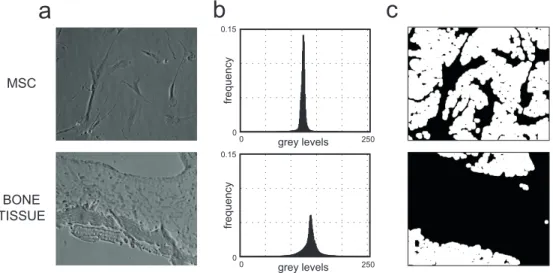
To estimate the vignetting function, we start by analyzing a sequence of im-ages acquired under the same microscopes set-up conditions. Ideally, an image can be always subdivided into two complementary regions, foreground and background, where the foreground usually represents the objects of interest. In optical microscopy, as already mentioned, the main part of the routine ex-amination is performed on cell culture or histological samples. Accordingly, as the foreground we consider cells and tissues and as the background cul-ture medium and glass, respectively (Fig. 2.3). It is worth noticing that the background is widely homogeneous compared to the foreground and using a homogeneous object to estimate the vignetting function is trivial, since the brightness intensity curvature is directly proportional to this function.

The fundamental step of the proposed method is the dense background re-construction achieved through a nonparametric approach. The images of the

a

b

c

Fig. 2.3: Background segmentation. (a): two phase contrast widefield images: the first is related to a cell culture of mesenchymal stem cells (top), the second to a histological sample of a bone tissue (bottom). The contrast of the images has been stretched to improve visualization. (b): frequency of intensity levels of the images reported in Fig. 2.3a. In x the intensity values in grey levels. In y, the frequency values. In these types of images, the values of background and foreground lie in the same range. Thus, it is not possible to separate background from foreground using common approaches related to histogram analysis. (c): background image masks (in white) in Fig. 2.3a. These masks are obtained exploiting the proposed method to detect and segment the background values using a spatial approaches based on the first derivative.

sequence are first stored into a stack and the background is detected using a segmentation step based on the first derivative. Uncertain pixels, like those near the foreground regions, are discarded. A subsequent z -median filter is performed on the extracted regions and the obtained curve can be consid-ered a good reconstruction of the background. Finally, in order to attenuate the noise typically present in the acquired images, a final spatial filtering is performed. The vignetting function is then estimated starting from the recon-structed background and subsequently normalized to the mean value of the obtained curve (see the algorithm pipeline highlighted in Fig. 2.4)).

In this approach, two particular stages must be analyzed in detail: the back-ground segmentation, based on the first derivative of the single images, and the dense background reconstruction, necessary in case holes are present due to groups of (x,y) pixel position not having any correspondent background value.

Fig. 2.4: Algorithm pipeline. Schematic flow chart of the proposed algorithms pipeline. Sequence acquisition: the method is multi-image based and exploits a sequence of images acquired under the same system set-up. Background segmen-tation: based on the first derivative mask. Background reconstruction: to obtain a dense surface though a z -median filtering and a low-order fitting. Vignetting estimation: to perform a spatial filtering of the dense background followed by a final normalization. Images correction: standard flat-field correction.

2.3.1

Background segmentation

Typically, to segment the background by excluding the foreground, the images histogram is analyzed to look for bimodalities and to see if two distributions exist that can be separated. In this case, several local [92, 93] or global [94] methods are used to define a suitable threshold value. Unfortunately, these ap-proaches do not provide effective results if there is a large overlapping between the value distributions of background and foreground, which often happens in low contrast brightfield images (Fig. 2.3b).

To avoid these problems, in the proposed algorithm the histogram analysis of the original image is left out in favor of a spatial analysis: the assumption that in widefield microscopy the background is quite homogeneous yields the values of the first derivative in the backgrounds regions always lower than those in the foreground. Accordingly, the algorithm extracts the image background regions through analyzing the first derivative. Typically, not only the objects borders express a high first derivate, but also the objects internal structures can have values higher than the background. By processing the derivative masks through applying a global threshold, a subsequent strong morphological opening and a final removal of small size regions (area filtering), it is easy to obtain reliable masks where the presence of foreground and uncertain pixels is negligible (Fig. 2.3c). According to this approach, detecting all the background pixels is not crucial; what is fundamental is that all the pixels definitively detected, except a negligible number, belong to the background. However, at the same time we have to include enough background pixels so that the final reconstruction is dense.

Therefore, we have devised a strategy to achieve a suitable threshold value Th for derivative, that yields a good trade-off. To this purpose, we started by computing the mean value of the first derivative in a ROI manually selected from the image background. Subsequently, we chose for Th three times the value estimated that experimentally has been shown to be a suitable choice. Furthermore, it is worth remarking that this value is not too sensitive: using lower values (e.g., the double) could only yield slightly larger holes in the background masks.

2.3.2

Dense background reconstruction

One of the most important step of the proposed algorithm is the reconstruction of the dense 2D background surface. This stage is basically composed of three main operations:

• extraction of the background regions from all the single images of the sequence,

• calculation of the mean value for the (x,y) pixel positions using the pixel labeled as background only,

• closing any remaining holes due to lack of background in those (x,y) pixel positions.

In particular, the last step is required if some (x,y) pixel positions exist where no image contains background. In this case, the obtained curve would not be dense and would contain several holes. For instance, this happens when using images of a cell culture with 100% confluence (with the term confluence we mean the percentage of the area occupied by “objects”, i.e., not background. 100% confluence means completely full of cells).

To avoid this problem, the simplest solution is to ask the operator to acquire more images until each (x,y) pixel position of the entire area is covered with enough backgrounds contributions. When this is not possible, such as when the images are processed off-line, a fine choice is fitting the nondense 2D back-ground surface with a low order polynomial and filling the holes with the estimated data without altering the values in the dense regions. Choosing a

low order polynomial is the best choice because the vignetting function typi-cally assumes quite a regular trend: as a matter of fact, strong local changes can be attributed to lens impurities or dust. Nevertheless, to infer this miss-ing information in correspondence of holes is almost always possible. That is, fitting gives good results only if holes are small and sparse. Otherwise, in case of too large holes, the lack of data would require parametric methods and our approach would lose its applicability.

2.4

Materials and tools

To test the method, 2 synthetic and 4 real-world image sets of different con-tents have been used. The synthetic images reproduce cell cultures at different confluences (60% and 80%). The real-world images regard living Mesenchymal Stem Cells (MSC), living Human Embryonic Kidney (HEK) cells and fixed his-tological specimens of bone and lung tissues. The cell cultures were contained in commercial plastic six-well plates and the histological tissues were placed on glass slides with mounting medium. The confluence of the MSC images used in the experiments was about 30%. All the images were acquired employing a diffused non automated widefield microscope, where the K¨ohler alignment is performed periodically. In particular, we used an inverted Nikon Eclipse TE2000-U endowed with a Nikon DXM1200 charge-coupled device (CCD) cam-era. The vision sensor is a 2/3” CCD, with approximately 1.3 Mpixels, square, with 6.7µm side. The response function is almost linear, as it happens for most of the present industrial CCD cameras coupled with microscopes. The images were acquired either in phase contrast or brightfield. The objective used was always a Nikon Plan Fluor 10×/0.30 Ph1 DLL ∞/0.17, a standard lens char-acterized by 10× magnification factor with a numerical aperture of 0.30 and the phase plate mounted in the lens focal plane. To acquire brightfield images no additional component was used, whereas the corrected condenser annulus diaphragm (Ph1) was aligned during the acquisition of phase contrast images. The final image size was fixed at 512×640 pixel resolution, and the images were saved as Bitmap (BMP format, RGB, 8-bit/channel). Each acquired im-age was then converted to grayscale using two open source imim-age processing software widely cited in literature: ImageJ [95, 96] and GIMP ( c The GIMP Team, [97]). The algorithm is written in MATLAB ( c The MathWorks, Inc., Massachusetts, USA) and it is distributable upon request [11].

2.5

Experimental results

The experiments aim at assessing the improvements that the proposed method described above yields in terms of vignetting removal: the outcome is com-pared with those achieved by flat-field correcting the images using reference vignetting functions obtained from EF, culture medium free of cells and glass slide without any tissue.

Five different types of experiments were performed.

First, the method was assessed using different images, manually segmented by an expert operator, in order to get the backgrounds “ground truth”. The term “ground truth” is typically used in Pattern Recognition, mainly in supervised classification tasks, to define the pattern being considered as the true one. Hereafter, the definition is also extended to Image Processing mainly referring to the output of a manual segmentation task.

Second, the vignetting functions, estimated using stacks of synthetic images, and the ground truth ones, were statistically compared to evaluate how the confluence and the number of images could affect the reconstruction.

Third, the shapes of the vignetting functions, estimated using stacks of real world images, were compared with those of the reference vignetting functions. Fourth, the flatness of the background of some representative images belong-ing to the real world sequences was evaluated before and after the flat-field correction, performed using the estimated and reference vignetting functions, according to the formula of Eq. 2.2.

Fifth, although the improvements in removing the vignetting effect yielded by our flat-field correction method can be perceived visually, they were even measured on both background and foreground, using sequences of overlapping images in mosaics.

2.5.1

Experiment 1: quality of the background

segmen-tation

The goal of the proposed background segmentation is to detect the background while minimizing the false positive pixels. This means that discarding several background pixels is acceptable. The goal is that the pixels finally labelled as background ones are reliable, almost without any foreground pixels erroneously included in the segmented region. To prove the specificity of the background segmentation, the foreground ground truth of the representative images, re-lated to different cell cultures and histological specimens, was obtained through a manual segmentation performed by an expert operator. It is worth noting that manual segmentation is a very time consuming task. For each image, the background automatically segmented with the proposed method and the foreground ground truth was compared. Of course, the best result is to obtain a background mask where no foreground pixels are included. In practice, this means that there should not be any overlapping region between the foreground mask manually segmented and the background mask obtained automatically. To this purpose, the results regarding 4 different images, representative of those achievable with a widefield microscope in phase contrast or brightfield, are presented. In particular, these few images are really representative as the whole sets used because in cell culture images the main feature is represented by a very low contrast culture medium, while each histological sample shows the same texture in the whole specimen as far as the uniformity of background is concerned. The first image represents a culture of MSC (Fig. 2.3a top), the second regards fixed unstained bone tissue (Fig. 2.3a bottom), the third refers to HEK cells (Fig. 2.5a top) and the last regards lung tissue stained with Hematoxylin and Eosin (Fig. 2.5a bottom). In particular, the first two images are characterized by quite a general low contrast.

The first two columns of Tab. 2.1 report the threshold values of the first im-age derivative yielding 1% and 5% of foreground pixels erroneously detected as being background (false positives). Regarding the parameters of the pro-posed segmentation algorithm, in all the experiments we used a disk-shape kernel (morphological structuring element) with 9 pixels radius for morpho-logical opening and then removed the regions smaller than 15×15 pixels. In particular, the MSC images are typically characterized by a very low contrast,

a b c HEK CELLS LUNG TISSUE AUTOMATIC SEGMENTATION MANUAL SEGMENTATION d DIFFERENCES

Fig. 2.5: Comparison between automatic and manual background segmentation. (a): images of HEK cells (top) and a lung tissue histology (bottom). The con-trast of the images has been stretched to improve visualization. (b): background masks (in white), obtained using the proposed automatic background segmentation algorithm: the percentage of false positive is below 5%. (c): reference masks of background manually segmented by an expert microscopist. (d): images represent-ing in different colours the differences between the masks obtained manually and automatically. In green the pixels where the masks present both background or both foreground values. In blue the pixels where the mask automatically obtained presents foreground and the mask manually obtained presents background values. In red the false positive pixels where the mask automatically obtained presents background and the mask manually obtained presents foreground values. Only few pixels for each figure result red.

threshold value [gray levels] mean of the first derivative set limit false limit false area 1 area 2 area 3

positive < 1% positive < 5%

MSC 5.5 7.5 2.2 2.1 2.1

HEK 22.5 37.5 2.4 2.2 2.3

BONE 8.5 11.5 2.3 2.2 2.3

LUNG 8.5 27.5 2.1 2.2 2.2

Tab. 2.1: Threshold values for the background segmentation. The foreground pixels erroneously included in the background masks (false positive) were counted using four different types of images depicting: MSC, HEK cells, bone tissue, and lung tissue. To this purpose, the masks obtained using the proposed algorithm to automatically detect and segment the background were compared with the ground truth. The first two columns report the first derivatives threshold value yielding a false positive rate of 1% and 5%. The last three columns report the mean values of the first derivative, calculated in three background ROIs manually selected.

even when acquired in phase contrast, mainly due to their nature of being flat adherent cells, therefore tending to settle in a very thin layer. For

compar-ison purposes, we acquired two images of nuclei and actina filaments, both referring to adherent cells, that is MSC and osteosarcoma bone cells (Saos-2 by ATCC, coming from standard commercial line, catalog no. HTB-85) using Nikon Eclipse Ti confocal microscope equipped with a digital CCD DS-QiMC camera and a Plan Apo VC 60× Oil DIC N2 lens (Fig. 2.6). In these types

a

b

c

d

Fig. 2.6: Depth dimension of Mesenchymal Stem Cell. Comparison between fluo-rescence images regarding Mesenchymal Stem Cells (MSC) (a, c) and osteosarcoma bone cells (Saos-2) (b, d), acquired at 60× using a confocal microscope. The cells nuclei are highlighted in blue, using DAPI, while in green the Actina filaments us-ing FITC. (a) and (b) are 3D plots of the acquired stacks of slices. Images (c) and (d) report the top view and the (x,y) depth projections of the volume maximum intensities. The depth dimension of the MSC is about half of the Saos-2: 3.9µm and 8.1µm respectively.

of images, it is quite difficult even for an expert biologist to manually segment the foreground. This is the reason why the lowest values, reported in the first two columns of Tab. 2.1, are related to the MSC images. A derivative

thresh-old value T h = 7.5 (expressed in gray levels) was experimentally proved as being the minimum value to obtain in each image a maximum false positive rate of 5%, which could be more than an acceptable value. Furthermore, it is worth noticing that for all the images used in the test, except for the MSC images, the false positives related to this threshold value are lower than 1%. As mentioned before, to define a fair threshold value for the first derivative, a correct strategy could be to manually segment some background ROIs in the image and to compute the mean of their first derivative. This value, multiplied by a positive correction factor, could be considered a good threshold. The last three columns of Tab. 2.1 report the mean values of the first derivative of three background regions, manually selected for each image. All the values are at least three times lower than T h = 7.5 (i.e., ≤ 7.5/3), hereafter chosen as the first derivative threshold for each image. Figs. 2.3c and 2.5b report the back-ground masks determined using our algorithm and related to the four tested images.

2.5.2

Experiment 2: vignetting estimation in function

of number of images and cell confluence

As already stated in Sect. 2.3, the confluence of images affects the reconstruc-tion of the vignetting funcreconstruc-tion. For instance, the proposed method fails in case of images of cell cultures with 100% confluence, where no background region is present. To analyze how confluence and number of images of the processed stack affect the reconstruction, we employed some stacks of synthetic images where cell cultures are artificially simulated. The images were built using an image generator implemented in MATLAB. Cells and debris are simulated, over a flat background, by randomly displacing in the field of view two different types of chessboard. The number of cells and debris depends on the required confluence. The vignetting function we built artificially, with the purpose of setting up a ground truth in the subsequent simulations, is then applied by multiplication to the synthetic images obtained, followed by the application of Added White Gaussian Noise (AWGN) with mean 0 and standard deviation (std) 4. We used the grey levels image generator to obtain stacks of images with 512×640 pixel size at 60% and 80% cell confluences (Fig. 2.7a). In par-ticular, the higher confluence value was selected as an upper bound, because in real world cases obtaining good results using a stack of images with higher

1.5 0.5 in te n si ty [n .u .] x y

b

a

c

Fig. 2.7: Relation between vignetting, confluence and number of images. (a): a generated synthetic image characterized by a confluence value of 60%. (b): 3D plot of the biquadrate function used to simulate the vignetting in the synthetic images. (c): trends of the mean absolute difference between the vignetting functions esti-mated with the proposed method and the ground truth, related to the confluence and the number of images of the stack processed.

confluences is very challenging, due to the small percentage of background available. To build the images we used a perfectly flat background (gray value set at 85), while for cells and debris we used two different square-shape black and white chessboards (each black or white square of 2×2 pixels), with ex-ternal chessboards’s side of 51 and 3 pixels, respectively. The values could be considered representative for MSC and debris visualized using 10× microscope lens. The vignetting function was obtained using a 2D biquadric distribution (Fig. 2.7b) with normalized values ranging between about 0.5 and 1.5 and the maximum value in the center of the field of view. Finally, the vignetting func-tions, reconstructed using the proposed method and stacks of different number of images, were statistically compared with the vignetting function of ground truth by computing the pixel-wise mean absolute difference (the sign differ-ences would compensate with each other giving a mean values near to zero). For each confluence (60% and 80%) and number of images (we choose sets of 3, 5, 7, 9, and 11 images) we built five different stacks.

analyzed for each fixed number of images. Using lower confluence value (60%) the vignetting function estimated is very similar to the ground truth just using stacks of three images only. Using 80% confluence the results are expectedly worse, but with a stack of 7 images only the mean absolute difference with the ground truth is as low as 2%. These results prove that also when using high confluence images the proposed method is capable to excellently reconstruct the vignetting function, by always exploiting a very small number of images. The synthetic image stacks free of vignetting and noise are distributable upon request [11].

2.5.3

Experiment 3: comparison of shapes of different

vignetting functions

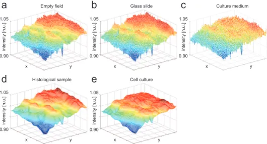
The goal of this experiment is to estimate how much the vignetting functions estimated from the images themselves resemble the reference ones. To this purpose, we used several sequences of images acquired in the same day, by using the same equipment set-up, including lamp voltage and exposure time. In particular, we propose the results obtained using two sequences of images: the first one is made of 13 images of a MSC culture, while the second one is of about 15 images of a histological sample of bone tissue. For each sequence, the percentage of (x,y) pixel positions is less than 2% where at least three images gave a background contribution. The vignetting functions estimated with the proposed method were compared with the reference ones estimated from EF, culture medium only and a part of a glass slide where no tissues are present. To obtain the reference vignetting functions, dozens of images were acquired for each of them and a simple z -median filtering was performed for each (x,y) pixel position. It is worth noticing that the sequence of 13 MSC images and the images referring to the culture medium only came from two different wells of the same commercial plastic six-well plate and the images related to the glass slide came from the same specimen slide of bone tissue cited above, but from regions free of tissue. To be able to compare the different functions, each of them is first normalized by its mean value (V iN). The Absolute Difference

Normalized Metric (ADNM), an absolute pixel wise subtraction between two different surfaces, normalized by the range interval of the first one (according to Eq. 2.3), has been computed between each normalized vignetting function

and the one estimated from the EF, normalized by its mean value (EFN).

ADN M (x, y) = kEFN(x, y) − V iN(x, y)k max(EFN) − min(EFN)

(2.3) The mean value and the std of the ADNM give us information about the relative discrepancy [98] of the different functions.

Fig. 2.8 shows the different vignetting functions used for comparison. The

1.05 0.90 1.05 0.90 1.05 0.90 1.05 0.90 1.05 0.90 in te n si ty [n .u .] in te n si ty [n .u .] in te n si ty [n .u .] in te n si ty [n .u .] in te n si ty [n .u .] x y x y x y x y x y Empty field Histological sample Glass slide Cell culture Culture medium

a

b

c

d

e

Fig. 2.8: Vignetting functions shapes. The first row reports the 3D plots of the surfaces of the vignetting functions estimated from: (a) EF, (b) glass slide free of tissue, (c) culture medium only. All these functions are obtained by performing a simple z -median filtering on a stack of acquired images. The second row reports the vignetting functions estimated from: (d) a histological sample of bone tissues, (e) a culture of MSC. The last two estimations were obtained using the proposed algorithm. All the functions were normalized to their specific mean value, so the z -axis of the 3D plots is relative to the normalized unit (n.u.) of the intensity values.

asymmetry is mainly due to the loss of the K¨ohler alignment. It is evident that the three reference vignetting functions (Figs. 2.8a and 2.8c) obtained using a simple z -median filtering are noisier than the two obtained using the proposed method (Fig. 2.8d and 2.8e). This is due to the fact that no spatial filtering was performed in the former functions. As a matter of fact, the following ranking based on the ADNM evaluation was expected. From best (smallest mean and std values) to worst results: vignetting function estimated from a glass slide

free of tissue, the histological sample with bone tissue, the cell culture, the culture medium without any cell inside. The reason why the best result was achieved with the glass slide is obvious: a glass slide and an EF behave almost in the same way as far as the transit of the light is concerned. For the same reason, one could expect the second best results for the histological sample: the proposed algorithm reconstructs the function starting from the background region and in a histological sample the background regions are glass regions free of tissue. The culture medium present in both cell culture and culture medium is a very different substrate from an EF: in this case, the light must cross a significant volume of medium and the lower plastic support of the wells plate. The worst result is the one obtained using the culture medium only, without cells inside, because the vignetting function estimated from it was obtained with a simple median z -filter, without any segmentation step that removes the debris present in the medium. Instead, the algorithm performed in the second sequence, the one referring to the cell culture, contains a segmentation step where both cells and debris are removed: in this case the vignetting function is estimated from a less noisy subset of pixels. Tab. 2.2 reports the mean value and the std of the ADNM computed for each V iN obtained.

ADNM set mean [%] std [%] GLASS SLIDE 3.20 2.18 BONE TISSUE 3.35 2.67 MSC CULTURE 5.45 4.17 CULTURE MEDIUM 6.30 4.60

Tab. 2.2: The Absolute Differences Normalized Metric (ADNM, Eq. 2.3) was performed using the reference vignetting functions, estimated from EF images, and those estimated from: a glass slide without any tissue, a histological sample of a bone tissue, a culture of MSC, a culture medium without any cell inside. Columns report the percentage values of mean and std of the obtained ADNMs.

2.5.4

Experiment 4: effectiveness of image correction

using different vignetting functions

The flat-field correction, performed using the vignetting function, aims to com-pensate the fall-off of the images brightness. Theoretically, if the true function