A new approach for the dynamic modelling of the human knee

Università degli Studi di Bologna

FACOLTA' DI INGEGNERIA

Corso di Dottorato in

ING-IND/13: MECCANICA APPLICATA ALLE MACCHINE

Ciclo XX

A new approach for the dynamic modelling

of the human knee

Tesi

di

Dottorato

di:

Coordinatore:

Ing.

Nicola

Sancisi

Chiar.mo

Prof.

Vincenzo

Parenti

Castelli

Tutore:

Chiar.mo Prof. Vincenzo Parenti Castelli

Chapter 1 Introduction 5

Chapter 2 The modelling of the human knee 9

2.1. Anatomy of the knee . . . 9

2.1.1. The knee components . . . 9

2.1.2. The description of the knee motion . . . 12

2.2. A novel procedure for the knee modelling . . . 13

2.2.1. The sequential approach . . . 13

2.2.2. The passive motion of the knee . . . 15

2.2.3. The in vivo feasibility of the basic tasks . . . 16

2.3. First step: the model of the passive motion . . . 17

2.3.1. The model of the tibio-femoral joint . . . 20

2.3.2. The model of the patello-femoral joint . . . 23

2.4. Second step: the stiffness model . . . 28

2.4.1. The multi-fibre model . . . 29

2.4.2. An alternate approach for the contact modelling . . . 35

2.5. The further steps . . . 39

Chapter 3 The definition of model parameters 41 3.1. The acquisition of the anatomical data . . . 41

3.2. The identification procedure . . . 46

3.2.1. The first approximation of the models . . . 47

3.2.2. The optimization procedure . . . 49

3.3. Results . . . 55

Chapter 4 Conclusion 61

Introduction

The study and the analysis of the human knee is a particular sector of Orthopaedics which has constantly attracted the attention of researchers. The huge number of surgical operations which every year are devoted to total or partial articular re-placements is an index of the importance acquired within the scientific commu-nity. Thus, it is not surprising that the growing attention on this field of research has recently exceeded the bounds of Orthopaedics and involved those of Physics, Mathematics and Engineering.

Great attention has been devoted in particular to the modelling of the knee. Models which can accurately reproduce certain characteristics of this joint are im-portant tools which help to understand or to discern many functional aspects that could be difficult to observe by means of standard experimental analyses. The forces exerted by the muscles and by the other articular components of the knee are a clear example of the difficulties which can be found within the practice: the experimental procedures and tools which are now available to measure these forces are highly invasive and do not make it possible to obtain the required information. Nevertheless, the knowledge of the knee articular forces could be a support for clinical diagnoses and analyses; furthermore it could provide significant insights on the field of prostheses and orthoses [6].

As regards this point, knee models prove useful also as effective tools for the aided design of innovative prostheses and orthoses. This is not only the result of the amount of information which can be obtained easily and quickly from a model. As in other applications, knee models make it possible indeed to reduce the cost of the prototyping stage, since they allow designers to foresee the behaviour of a prosthesis or an orthosis once it has been implanted on a patient. Moreover, the use of models during the design stage would reduce the number of experimental tests which should be carried out in vivo or in vitro to optimize a particular design or to fit the patient characteristics.

Knee models also are fundamental instruments in the surgical planning of an operation or during the operation itself. Some models are used jointly with medical devices to customize or to modify prostheses and orthoses on an individual patient.

Furthermore, as in prosthesis design, knee models allow surgeons to foresee the behaviour of a prosthetic knee, in particular when the original articular components are modified or removed at all. Finally, the use of efficient models could reduce the experimental tests on the patient and the post-operation interventions.

Many models have been presented in the literature as a confirmation of their scientific and practical relevance [16]. Starting from the early bi-dimensional mod-els [8, 21, 27, 35] and arriving at the recent three-dimensional ones [5, 15, 17, 19, 31, 37, 38, 45], the accuracy of the mechanical description of this articulation has constantly grown. In some cases these models have been defined from average data taken from the literature, otherwise they have been based on experimental data, trying to fit a particular required task.

In the last few years, many models have been proposed for the dynamic mod-elling of the knee joint [6, 16]. Their common target is to replicate the relative motion of the three main bones of the knee (i.e. the tibia, femur and patella) when a known set of forces are applied to the joint. Sometime the forces are time-dependant: this is the typical situation studied by the authors which model the motion of the knee during specific but significant tasks, such as during normal walking or rising movements [30, 31, 35, 41, 42]. Other studies examine the be-haviour of the knee when static or quasi-static forces are applied, to obtain the equilibrium configurations of the joint [2, 4, 15, 17, 23, 26].

The final objective of all these studies is to define a model that fit a particular task. Many strategies have been devised to reach the target, but a common pro-cedure could be outlined. This is what could be called a simultaneous approach: starting from a set of data obtained from the literature or from an experimental ses-sion, some elements of the knee are modelled, others are ignored; the parameters which define the knee model as a whole are identified in order to fit experimental results or medium values reported in the literature. The main differences between the models lie in the number of considered elements, in the model of each element and in the optimization approach used to fit the experimental results.

The simultaneous approach makes it possible to obtain models which can ac-curately replicate the relative motion of the tibia, femur and patella for a specific task. Unfortunately, the specificity of the task respect to which the models are identified represents also the main drawback and the fundamental limitation of this approach. The optimization of all parameters with no particular distinction among them makes sure that the functional and stabilising role of each structure of the knee is somehow lost. In other words, the basic function of each structure is not replicated in general in the model. As a result, the optimized model can simulate the knee motion during a given task, but nothing can be said a priori when other tasks are prescribed, or when the loading conditions of the joint are altered.

The main consequence of this drawback is that if these models can be useful and reliable to obtain data which could not be recorded in an experimental session (such as muscular or other articular forces), at the same time they present strict limitations for the planning of an operation or for the prosthetic design. These applications indeed have no fixed tasks; moreover, they require models which allow

one to foresee the behaviour of the joint when the original conditions are modified. The aim of this dissertation is to propose a novel approach for the dynamic modelling of the knee. The proposed procedure is directed to overcome the prob-lems and limitations connected with the simultaneous approach. The dynamic model of the knee is defined gradually, by passing through a sequence of steps, i.e. of intermediate models, which allow the anatomical function of each structure of the joint to be correctly replicated. In particular, the procedure makes it possible to assign each articular component its correct role which, as a consequence, can be easily identified. The fundamental rules of the novel approach make sure the stabilizing role of these structures is preserved step after step, until the final model of the joint is obtained. The target of the new approach is to define models which can be useful and reliable also for those applications, such as the surgical planning and the prosthetic design, which cannot rely on specific tasks in general.

In order to prove the potentialities of the method, the new approach is exploited to define a stiffness model of the knee. This model can replicate the behaviour of the joint when external quasi-static forces are applied. The point of originality of the model lies on its gradual definition: a purely kinematic model is defined at first, in order to replicate the natural motion of the knee when no loads are applied to the joint; this model is then enriched with new elements which make it possible to extend the application of the model to quasi-static loading conditions.

The new approach and the theoretical and anatomical foundations of the model are presented in chapter 2. In order to show the accuracy of the model and the efficiency of the proposed procedure, the model is synthesized from experimental data in chapter 3 and the results are compared with those obtained both during an experimental session and with data published in the literature.

The modelling of the human knee

The new approach and the theoretical and anatomical foundations of the knee model defined in this dissertation are presented in this chapter. A brief anatom-ical section introduces the main matter; the most important aspects of the proposed procedure are then described in section 2.2; finally, in sections 2.3 and 2.4 it is shown how to apply the procedure for the modelling of the human knee.

2.1

Anatomy of the knee

This section gives some basic information about the knee. Its scope is to describe the anatomical structures that are considered in the following. Furthermore, the nomenclature and the conventions adopted in this dissertation are presented. This paragraph is not meant to be a complete treatise about the human knee, but a short and simple reference to clarify those points which are used in this dissertation.

2.1.1 The knee components

The knee is a joint which allows the relative motion between three bones of the leg, i.e. the tibia, femur and patella (Figure 2.1). A forth bone, i.e. the fibula, is connected to the tibia by a strong but not rigid connection; anyway, the relative movements between the tibia and fibula will be ignored in this dissertation, since they are irrelevant as it will be clear in what follows. Two sub-joints could be rec-ognized: the tibio-femoral (TF) and the patello-femoral (PF) joints, whose names come from those of the bones which enter into mutual contact during knee mo-tion. As regards TF, two tibia proximal surfaces (i.e. the tibial condyles) move on two femur distal surfaces (i.e. the femoral condyles). As regards PF, the patella can slide on the femoral condyles and on the trochlea, i.e. the antero-distal sur-face of the femur between the condyles. The contacts between the femur and tibia actually are partly mediated by two cartilaginous elements, i.e. the menisci. The menisci are not considered in the model described in this dissertation; anyway, this simplification does not constitute a limitation of the proposed procedure.

(a) Lateral view. (b) Back view.

Figure 2.1: A lateral view (a) and back view (b) of the knee. The main structures which constitute the joint are represented [34].

The knee is formed by several anatomical parts which will be called structures, elementsor components in the following, without distinction. They can be divided into passive and active structures. Passive structures are those elements which can exert forces only if externally stressed: articular surfaces, menisci, ligaments and other ligamentous structures belong to this category. On the contrary, active structures — such as the muscles — can intrinsically exert forces but, in general, they almost do not oppose external forces when inactive.

Articular surfaces are those parts of the bones which enter into mutual con-tact during knee motion. In this case, they are the tibial and femoral condyles, the trochlea and the dorsal (or back) surface of the patella. Since the femoral condyles are two distinct surfaces, sometime they will be called the medial and lateral condyle; the same remark holds for the tibial condyles as well.

Ligaments are very important knee elements which have a strong influence on the stability of the joint. They are composed by a fibrous connective tissue; that is why when only a part of the ligament is considered, it is referred to as a fibre or a bundle of fibres. The most important ligaments of the knee provide a bone-to-bone interconnection between the tibia, fibula, femur and patella. The connective area between a ligament and a bone will be called attachment or attachment area in the following, without distinction. Thus, the two attachments of a certain ligament could be called the femoral and tibial attachments, for instance.

The four major ligaments which interconnect the tibia-fibula complex and the femur are the anterior cruciate (ACL), the posterior cruciate (PCL), the medial collateral (MCL) and the lateral collateral (LCL) ligaments; the patella is con-nected to the tibia by means of the patellar ligament (PL). Photographic images of these ligaments are presented in Figure 2.2: they were taken from a specimen,

(a) The cruciate ligaments. (b) The patellar ligament.

(c) The medial collateral ligament. (d) The lateral collateral ligament.

Figure 2.2: The principal ligaments of the knee joint.

during an experimental section carried out at the Movement Analysis Laboratory of the Istituti Ortopedici Rizzoli (IOR) (section 3.1). Other ligaments considered in this dissertation constitute the so-called posterior structures of the knee, since they interconnect the posterior part of the tibia-fibula complex and that of the fe-mur. They are the arcuate ligament, the popliteus tendon and the oblique popliteus ligament. Even if the popliteus tendon is not technically a ligament, it can exert passive forces due to its particular connection to the bones [43].

Knee muscles are not modelled in this dissertation, but only the quadriceps is presented here. It is the main muscle of the knee and it is made up of four distinct portions. All of them are attached to the patella on one side by means of the patellar tendon; on the other side, some portions are attached to the femur, while the others to the ilium.

2.1.2 The description of the knee motion

In order to identify every point of the joint, it is necessary to define reference frames. In particular, it is convenient to define three anatomical frames attached to the tibia, femur and patella respectively: the coordinates of a point of a bone expressed in the corresponding anatomical frame do not change with knee config-uration. Moreover, the relative pose (position and orientation) between two bones can be described by means of the kinematic parameters which define the relative poses of the corresponding reference frames. Since the fibula is considered as rigidly attached to the tibia, these two bones share the same anatomical frame.

The three anatomical frame are represented in Figure 2.3. The tibia anatomi-cal frame (St) is defined with origin coincident with the tibia centre (on the tibial plateau); x-axis orthogonal to the plane defined by the two malleoli and the tibia centre, anteriorly directed; y-axis directed from the mid-point between the malle-oli to the tibia centre; z-axis as a consequence, according to the right hand rule. The femur anatomical frame (Sf) is defined with origin coincident with the mid-point between the lateral and medial epicondyles; x-axis orthogonal to the plane defined by the two epicondyles and the head of femur, anteriorly directed; y-axis directed from the origin to the head of femur; z-axis as a consequence, according to the right hand rule. Likewise, the patella anatomical frame (Sp) is defined with origin coincident with the mid-point between the lateral and medial apices; x-axis orthogonal to the plane defined by the lateral, medial and distal apices, anteriorly directed; y-axis directed from the distal apex to the origin; z-axis as a consequence, according to the right hand rule.

A relative pose of the femur with respect to the tibia can be expressed by means

−20 −10 0 10 20 30 40 50 60 70 0 10 20 30 40 −30 −20 −10 0 10 20 30 y z x Sf St Sp

Figure 2.3: The three anatomical frames St, Sf and Sp (orange) represented together with the tibial (blue), femoral (black) and patellar (red) articular surfaces.

of the position Ptf of the origin ofSf inSt, and by means of the 3x3 rotation matrix Rtf for the transformation of vector components fromSf toSt. Matrix Rtf can be expressed as a function of three rotation parameters α, β and γ:

Rtf=   cαcγ+ sαsβsγ −sαcγ+ cαsβsγ −cβsγ s_αc_β c_αc_β s_β c_αs_γ− s_αs_βc_γ −s_αs_γ− c_αs_βc_γ c_βc_γ   (2.1)

where c and s indicate the cosine and sine of the angle in subscript and α, β , γ represent the flexion, ab/adduction and intra/extra rotation angles of the femur relatively to the tibia, using a convention deduced by the Grood and Suntay joint coordinate system [13]. According to this convention, flexion is a rotation about the z-axis of Sf, intra/extra is a rotation about the y-axis of St, ab/adduction is a rotation about a floating axis, perpendicular to the previous ones. Positive signs of α, β and γ correspond respectively to femoral flexion, adduction and external rotations. Expression (2.1) can be applied for right legs; in order to use the same matrix for left legs, the signs of β and γ should be inverted in (2.1). Likewise, the matrix Rf p and the vector Pf p express a relative pose of the patella with respect to the femur; the matrix Rf pcan be represented by an expression similar to (2.1). Even though the Grood and Suntay convention was originally defined for the tibio-femoral joint, its application on different joints (the patello-tibio-femoral joint included) is becoming ordinary in the scientific literature.

2.2

A novel procedure for the knee modelling

2.2.1 The sequential approach

The main limitations of the simultaneous approach applied to the knee modelling have been presented in chapter 1. The simultaneous identification of all the model parameters does not guarantee that the functional and stabilising role of the articu-lar structures is correctly replicated within the model. As a consequence, the opti-mized model can simulate the knee motion during a given task, but if the loading conditions are changed the model could not be reliable any more. This drawback limits the use of the model for applications which have no fixed tasks and which require models to foresee the behaviour of the knee when the original conditions are modified.

It is clear that the perfect solution would be the definition of a model which could be accurate and reliable for every loading conditions. This is probably a dream at the moment, but the simultaneous approach does not seem the proper procedure to try to reach this target, for all the reasons which have been pointed out. On the contrary, it could be more promising to start building the model from its foundations, trying to fit as best as possible simple but basic tasks. These ba-sic tasks are particular loading conditions which emphasize the restraining role of certain elements of the knee; they should be simple since they should show the

Experimental data Model parameters Optimization Final model Experimental data Model parameters 1 2 … f Model 1 Optimization 1 Optimization 2 Model 1 Optimization f Model 2 Model 1 Model 2 Model f

(a) The simultaneous approach.

Experimental data Model parameters Optimization Final model Experimental data Model parameters 1 2 … f Model 1 Optimization 1 Optimization 2 Model 1 Optimization f Model 2 Model 1 Model 2 Model f

(b) The sequential approach.

Figure 2.4: Comparison between the simultaneous (a) and the sequential ap-proach (b).

stabilizing role of a limited number of structures at a time, making it possible to recognize those parameters that do not influence a certain behaviour of the joint. In this sense these tasks are an important foundation of the model and thus they should be used as a reference: they make it possible to model only those structures at a time which guide a particular basic motion of the knee.

The articular components are sequentially added to the model, in order to fit more and more complex tasks: the model grows from its foundations and the sta-bilizing roles of each element of the joint is emphasized. Moreover, the model becomes more and more sophisticated, making it possible to replicate the motion of the knee even under complex loading conditions. In order to make sure the function of each structure is preserved, it is fundamental that the addition of new elements does not interfere with the motion of the knee during previous simpler tasks. This is the most important condition to guarantee that, when the knee is sub-jected to the loading conditions of a basic task, only determinate elements could affect the joint motion.

This particular procedure will be called sequential approach in this disserta-tion, in contrast with the simultaneous approach described before. A comparison between the two procedures is shown in Figure 2.4. While in the simultaneous

approach the knee model is defined by means of one large-scale optimization only — preceded or followed by few small adjustments to the model parameters —, in the sequential approach the model is defined by means of a sequence of partial op-timizations which lead to a more and more sophisticated model, till the final one is obtained. In a certain sense, the final model is built starting from a basic block; other blocks are then added, until the final building is completed.

From an operative point of view, the sequential approach makes it possible to identify the model parameters by means of a number of sequential steps. At each step only some parameters are identified, satisfying fundamental anatomical constraints and characteristics of the knee.

The procedure is based on two important rules to achieve this objective: 1. Once a parameter has been identified at a particular step, it is not changed at

the following steps;

2. Parameters identified at each step must be chosen so that they do not alter the results obtained at the previous steps.

These two rules guarantee that the results obtained at each step do not worsen those already obtained at previous steps and, most importantly, they make it possible to choose new parameters of the model respecting the anatomical constraints satisfied at previous steps. The stabilizing role of the knee elements is so preserved, as new elements are added at each step.

In this sense, the proposed sequential approach is substantially an inductive procedure which starts from the definition of a simple model which can replicate the behaviour of the joint under very strict loading conditions. This preliminary model is then enriched, i.e. made more sophisticated, at each step, in order to obtain a more and more generalized model which can replicate the behaviour of the knee under more and more generic and complex loading conditions.

2.2.2 The passive motion of the knee

The sequential approach is only a partial aspect of the novel procedure which is proposed in this dissertation for the modelling of the human knee. It is indeed evident that the sequential approach needs a starting point, i.e. a preliminary model which can satisfy a first basic task and which represents the foundation of the final model. Being the first block of the procedure, the choice of the first basic task and its modelling are both crucial points for the complete knee model.

It is proposed here to choose the passive motion of the knee as a starting point of the sequential approach. The passive motion of the knee is the relative motion of the tibia, femur and patella when no loads (external or muscular) are applied to the joint. Experience shows that when no loads are applied to the knee, the joint does not have a single, well defined equilibrium position; on the contrary, the knee can assume an infinite number of possible configurations, all connected together.

This mobility is exactly the passive motion of the knee, i.e. the unresisted motion of the joint [10, 27, 45].

In a certain sense, the particular loading condition of the passive motion is the simplest one which can be exerted on the knee: this aspect meets the basic task requirement of simplicity and makes the passive motion a good candidate as a starting point for the sequential approach. This, however, is not the only reason which leads to choose the passive motion as the first step of the proposed procedure. Several studies [10] prove that knee stability is directly connected to the passive motion of the joint. As a direct consequence, a full understanding of this motion can provide significant insights on the role of the passive elements of the knee in the achievement of the joint stability. This is an important task for knee restoration and prosthetic design.

The passive motion is thus chosen as the first step of the sequential approach. The preliminary model of the knee — i.e. the result of the first step of the sequen-tial approach — replicates the passive motion only and includes only the articular elements which affect this particular motion. Only model parameters associated to these elements are identified. It is thus important to discern which structures influ-ence the passive motion, in order to exclude the others; moreover it is fundamental to define an accurate and efficient preliminary model in order to provide the final model a good foundation.

2.2.3 The in vivo feasibility of the basic tasks

A further principle should be considered in the choice of basic tasks. The models which stem from each step of the sequential approach are defined by means of a number of parameters which have to be identified on experimental data. These data could be obtained from the literature or from a knee in vivo or in vitro.

Several authors (see, for instance, [24]) proposed procedures that make it pos-sible to model the knee or its structures by means of invasive experimental tech-niques. Those include cutting and separation of bone segments, dislocation of articular components, exsection of ligaments or other elements of the joint. These techniques are often a requirement in order to acquire the experimental data which are needed for the parameter identification of the models.

Invasive techniques allow researchers to obtain experimental data which could be very difficult — if not impossible — to acquire otherwise; therefore they are an important source for many research purposes. As regards knee modelling, invasive techniques are thus useful to define and identify models for research and theoret-ical applications. On the contrary, it is clear that invasive techniques cannot be used when the model has to be defined for surgical planning or prosthetic design. These applications indeed need data which have to be obtained in vivo and, as a consequence, they have to be acquired by means of experimental techniques as less invasive as possible.

The choice of the basic tasks should take this aspects into proper consideration: if the model has to be used for practical purposes, it must be possible to replicate

the basic tasks in vivo by means of non-invasive techniques. If this principle is sat-isfied, it is actually possible to identify the model on the experimental data recorded from a patient.

The procedure proposed in this dissertation makes use of basic tasks which satisfy this principle. As explained in section 3.1, it was impossible to carry out an experimental session in vivo due to technical limitations, and the experimental data were recorded from a specimen or taken from the literature. Anyway, having the opportunity, the same data could have been obtained by means of non-invasive techniques also. It should be stressed, for instance, that the passive motion of the knee could be obtained in vivo.

Section 2.2 presented the main aspects of the novel approach which is used in this dissertation to model the knee joint. The application of the proposed procedure is presented in next sections; in particular, it is shown how to apply the procedure in order to obtain a stiffness model of the knee, starting from a passive motion model. Moreover, some details are provided on how to apply the procedure in order to further generalize the knee model.

2.3

First step: the model of the passive motion

Several studies [10, 45] prove that the relative movement of the tibia and femur during passive flexion is a one degree of freedom (dof) motion: once the flexion angle is imposed to the articulation, the corresponding pose of the tibia with respect to the femur is defined, both univocally and experimentally replicable. The same result holds also for the relative movement of the patella and femur [1]: despite the patello-femoral joint (PF) is slightly more slack during passive flexion if compared to the tibio-femoral joint (TF), experimental results prove that for a given flexion angle of the knee the relative pose of the patella with respect to the femur is repli-cable. As a consequence, the patella also shows a one dof of unresisted motion with respect to the femur.

Most papers dealing with 2D [35] and mainly 3D [5, 15, 16] modelling of the knee joint in passive motion consider more or less complex models which comprise visco-elastic connections between the involved structures. These models may be interesting but are computationally expensive. Moreover the identification of the anatomical parameters (stiffness, viscosity,. . . ) may be critical.

A further and more important point leads to the conclusion that these models do not fit well with the proposed sequential approach. The point stems from the equilibrium analysis of the joint under unloaded conditions. Since no forces are exerted on the articulation, no forces can be exerted by the passive structures of the knee to satisfy the equilibrium of the system composed by the tibia, femur and patella. The internal forces due to the passive structures could be internally auto-balanced, thus invalidating the concept of totally unloaded condition, but these cir-cumstances would be extremely complex to achieve on the full flexion-extension movement, even considering friction between articular components. As a

conse-quence, the ligaments and in general the passive structures of the knee cannot be tight during passive flexion: they can reach the limit between laxity and tension at the most.

All these observations involve important anatomical constraints which must be considered and satisfied by the knee model: when no forces are applied to the model of the knee, the relative motion of the tibia, femur and patella must be a one dof motion and the passive structures of the knee must not be tight. The most important consequence is that visco-elastic properties have no influence on the passive motion of the knee; moreover there are some components of the joint which do not even guide the passive motion, since they cannot exert forces being lax. These components can thus be ignored in the model of the passive motion: as explained in section 2.2.2, this model must include only the elements that affect this motion, and only the parameters which have an influence can be identified. This is a fundamental aspect of the sequential approach and this is why the models proposed in the cited studies cannot be used with the proposed procedure. Thus, a different approach should be followed for the modelling of the passive motion.

This approach stems from static-kinematic considerations [27]. Since knee flexion is guided along a one dof motion despite all its structures are slack or at the limit between tension and laxity, there exist some articular components which persist in this last status during the complete passive flexion: these structures are those which guide and that affect the passive motion. Furthermore, since no forces are applied to these components, they are subjected to no deformations. The funda-mental conclusion is that the passive motion of the knee can be modelled by means of a rigid link mechanism; the relative motion of the tibia, femur and patella can thus be obtained from the kinematic analysis of the equivalent mechanism.

The idea of equivalent mechanisms is not new and could be dated back to the classic four-bar mechanism (Figure 2.5(a)) [21]. Anyway the first

three-dimen-(a) The four-bar linkage. (b) A recent 3D model.

Figure 2.5: Two equivalent mechanisms of the tibio-femoral joint: the classic four-bar linkage [21] (a) and a recent 3D model [45] (b).

1 DoF

0 DoF

1 DoF

Figure 2.6: The two sub-chains of the passive motion model.

sional (3D) mechanisms which can replicate the motion of TF [45] (Figure 2.5(b)) appeared only recently in the literature. The first 3D equivalent mechanism which replicates the passive motion of the total knee (PF included) was recently presented in [38]. The main reason that led other authors to ignore the PF joint in the first 3D models is the partial independence of the TF motion with respect to the PF one: the passive motion of TF is independent from that of PF if tibia flexion is imposed. Thus the two sub-joints of the knee can be analysed separately and, in particular, TF can be modelled without taking PF into consideration.

The explanation of this aspect relies on the anatomical constraints between the two sub-joints. As explained in section 2.1, the patella slides on the femoral distal surfaces while it is connected to the tibia through the patellar ligament, and to the femur through the quadriceps. This muscle does not exert any forces on the patella during passive motion; moreover, the slight laxity of the quadriceps and the particular conformation of the joint make sure PF does not constitute a constraint to TF in this case. In other words, the patella moves on the femur surfaces being trailed by the patellar ligament.

It is important to note that, in order to respect the anatomical behaviour of the joint, the independence of the motion of TF from that of PF is not only an advan-tage, since it makes it possible to define the model of TF independently from that of PF, but incidentally it is also a requirement of the model of the complete joint. The knee model must show the same feature, to make sure it correctly replicates the anatomical constraints of the joint. As a consequence, the equivalent mecha-nism of the knee passive motion has to be composed by two sub-chains, i.e. two partial mechanisms, which show the requirement of partial decoupling. The first sub-chain is the model of TF and it must have one dof. The second sub-chain is the model of PF: it is connected to the previous one and it must have zero dofs. The complete mechanism exhibits one dof and the motion of the TF sub-chain is inde-pendent from that of the PF sub-chain if knee flexion is imposed. The Figure 2.6 clarifies this concept with planar mechanisms. The addition of a sub-chain with mobility zero to a mechanism does not change the mobility of the whole mecha-nism.

The two parts of the equivalent mechanism of the knee passive motion are presented separately in the following sections.

2.3.1 The model of the tibio-femoral joint

In the last few years, several mechanisms were presented which can accurately replicate the passive motion of TF by means of three-dimensional rigid link mech-anisms. Starting from the first one [45], a group of models was proposed which showed an increasing complexity [19, 33, 32, 28].

The geometric and kinematic observations which support these mechanisms are almost the same. Experimental analyses show that a bundle of fibres of the ACL, one of the PCL and another of MCL remain almost isometric during passive flexion. These bundles are called isometric fibres (IF). The other bundles of these ligaments are slack and reach the limit between tension and laxity at the most. Ar-ticular contact is preserved during passive motion: the medial and lateral femoral condyles enter into contact with the corresponding tibial condyles on two points (one for the medial and the other for the lateral compartments). All the other com-ponents of TF are slack and do not constrain the passive motion. As a consequence, the three IF and the two pairs of condyles are the only anatomical structures which guide and affect the passive motion of TF [44]. If the isometric fibres are assumed as truly isometric and the contacts are assumed to occur on two points, a 3D par-allel mechanism can be defined (Figure 2.7). This mechanism features two rigid bodies t and f (representing the tibia and femur) interconnected by three rigid bi-nary links A1B1, A2B2, A3B3 (representing the three IF); each link is connected to both rigid bodies by means of spherical pairs. Moreover, two surfaces attached to the first rigid body τ1 and τ2 (representing the tibial condyles) remain in con-tact with two surfaces σ1 and σ2(representing the femoral condyles) attached to the second rigid body. If the rotations of each binary link about its own axis are ignored, this mechanism shows one dof: the five constraints (the three links and

A1 A2 A3 B1 B2 B3

S

t

S

f t1 t2 s1 s2

Figure 2.7: The generic 3D parallel mechanism for the modelling of the TF passive motion.

the two contacts) remove one dof each from the relative motion of the two rigid bodies. Mobility and a synthesis procedure of this type of mechanisms have been investigated in [22].

The approximation of the model consists both of substituting the three liga-ments with the almost isometric fibres of the corresponding ligaliga-ments and of as-suming these fibres as truly isometric. Furthermore the condyles are approximated by lower-order surfaces that (two by two) move on each other, entering into contact on a single point per surface. The main difference among the models cited above is an even more accurate representation of the articular surfaces, while the concept of isometric fibres remains the same.

The increasing complexity of these models leads to a greater complexity of the corresponding mathematical models which define the kinematic analysis of the equivalent mechanisms. The kinematic analysis is the fundamental tool which makes it possible to obtain the relative motion of the tibia and femur by means of the equivalent mechanisms, as described in the introductory part of this section. In order to simplify computations, a further mechanism was recently presented that replicates the passive motion of the knee with a similar accuracy than the previous models, even if, reversing the common tendency, it is considerably simpler than the others [37]. This was possible by exploiting other kinematic properties of TF, with respect to the previous models. This model was proposed as a support for prosthetic design and for operation planning, in particular, since it allows faster and more stable computations, at the same time producing a mechanically simple solution.

A further reason which suggests to use models with a suitable complexity is that accuracy does not increase with complexity all the time. Numerical insta-bilities may arise indeed from the kinematic analysis of a too complex mecha-nism and the number of parameters of the model makes the identification from experimental results very difficult and time-expensive. The limitations of higher-order models were shown in [28]. The substitution of lower-higher-order surfaces with more complex ones did not produce particular benefits; on the contrary, the use of b-splines brought computational and optimization instabilities and the high order of the problem generated oscillations which, paradoxically, gave worse results than those of simpler models.

In a recent investigation carried out in [29], the approximation of the articular surfaces with spheres [33] proved very efficient for the modelling of the TF passive motion in analytical applications, providing a good balance between complexity of the model and accuracy of the synthesized motion. Thus, the same approxi-mation is adopted in this dissertation also. It is worth noting that this model is kinematically equivalent to a one dof 5-5 parallel mechanism, which features two rigid bodies interconnected to each other by 5 binary links, through spherical joints (Figure 2.8). The centres of the spherical surfaces on the femur are forced indeed to remain at the same distance from the corresponding centres of the spherical sur-faces on the tibia: the condyles can be substituted by two rigid binary links (similar to those representing the three IF) which connect two by two the centres of these

A1 A2 A3 A4 _A5 B1 B2 B3 B4 B5

S

t

S

f

Figure 2.8: The 5-5 parallel mechanism.

spheres. In conclusion, three out of the five rigid links represent the isometric fibres of ACL, PCL and MCL, while the other two — hereafter called as contact fibres (CF) — substitute the articular contacts between the medial and lateral condyles of the tibia and femur.

In order to obtain the passive motion of TF, the relative poses of the femur with respect to the tibia have to be obtained from the model for each prescribed flexion angle. Each pose can be expressed by means of the matrix Rtf and the vector Ptf: the first is the 3x3 rotation matrix for the transformation of vector components from Sf toSt; the second is the position vector of the origin ofSf inSt. Matrix Rtfcan be expressed as a function of three rotation parameters α, β and γ, as reported in equation (2.1). The required poses can be obtained by solving the closure equations of the 5-5 mechanism representing TF. As previously noted, these equations can be solved independently from those of the PF sub-chain since the relative motion of TF is not influenced by that of PF in passive flexion. The closure equations of the mechanism constrain each pair of points AiBi to keep the same distance at each imposed flexion angle:

Ai− RtfBi− Ptf

= L0i, (i = 1, . . . , 5) (2.2)

where points Aiand Biare the centres of spherical pairs, expressed inSt and inSf respectively (Figure 2.8) and L0iare the lengths of links AiBi; k·k is theL2_-norm of the vector. If the flexion angle α is assigned, (2.2) is a system of five equations in the five unknowns β , γ and Ptf components, which can be solved, for instance, by means of a quasi-Newton numerical procedure. The solution defines the relative pose of the femur with respect to the tibia for a given flexion angle.

The coordinates of the points AiinSt, those of the points BiinSf and the link lengths L0i (i = 1 . . . 5) constitute a set of 35 geometrical parameters which define

the TF model. The first step of the sequential approach consists in identifying the parameters of the passive motion model from experimental data; the identification of the geometrical parameters which define the TF model is the first part of this step. The procedure of identification — based on optimization — and the experi-mental session are described in sections 3.1 and 3.2. The parameters that define the structures which guide the passive motion of TF are thus determined as a result of this preliminary identification procedure. These parameters are not changed during the following steps, in order to observe the first rule of the sequential approach.

2.3.2 The model of the patello-femoral joint

A common characteristic of all the three-dimensional rigid link mechanisms for the modelling of the passive motion of the knee is that the patella is never consid-ered. This simplification stems from the observation that, in passive motion, PF has no influence on the relative motion of the femur and tibia, as explained in the introductory part of this section. On the contrary, as well known by experimental evidence and models presented in the literature [8, 17, 36], under different loading conditions the patella affects the TF motion during flexion: the stabilizing effect of PF on the loaded knee is a fundamental aspect of the joint mechanics which cannot be ignored. Thus, in order to define a passive model of the whole knee which can be used as a starting point for the sequential approach, the relative poses of the patella and femur must be known.

A few models which can replicate the passive motion of PF have been presented in the literature. Most of them consider deformations of the PF components and their visco-elastic properties [15]. The only rigid link mechanisms which have been proposed in the past for the modelling of PF are two-dimensional models of the relative motion of the femur and patella on the sagittal plane [8]. A 3D equivalent mechanism for the simulation of PF in passive motion has been presented in [38] only recently; in the same study, a 3D mechanism for the modelling of the passive motion of the whole knee has been proposed.

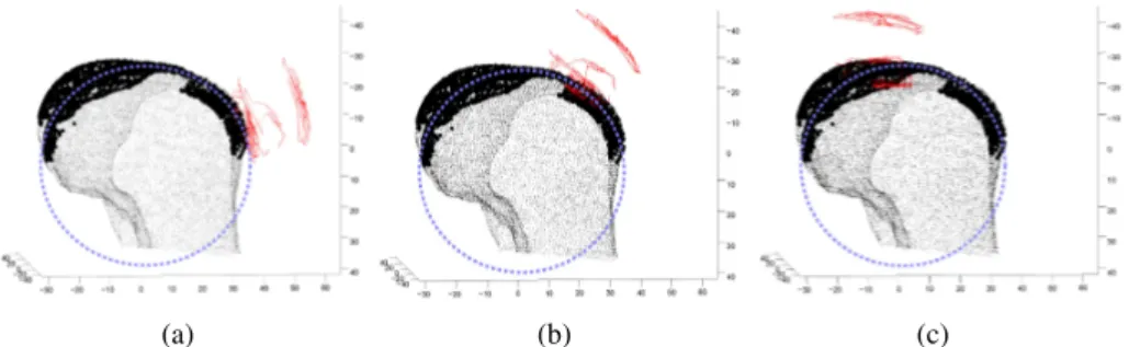
The equivalent mechanism of PF can be defined by means of anatomical and kinematical considerations about the relative motion of the patella and femur. The contact between the patella and femur occurs on a wide portion of their rigid ar-ticular surfaces for each flexion angle (Figure 2.9): this observation suggests that this contact can be modelled by means of a lower pair. In particular, the trochlea and the portions of femoral condyles which are involved in the contact can be ap-proximated by a cylinder. Thus, the relative motion of the patella and femur occurs about a fixed relative axis, i.e. the axis of the approximating cylinder. Moreover, the particular shape of the articular surfaces ensure that the patella has a limited mobility along the rotation axis: the dorsal surface of the patella fits — in a certain sense — the trochlea, the femoral condyles and the intercondylar space. These considerations all lead to the conclusion that the contact between the patella and femur can be modelled by a hinge joint which mutually connects the two bones. Furthermore, experimental observations show that a bundle of fibres of the patellar

(a) (b) (c)

Figure 2.9: The articular contacts between the patella (red lines) and femur (black points) at three different flexion angles. The cylindrical approximation of the condyles (blue circle) is also presented.

ligament remains almost isometric in passive flexion. This is a direct consequence of the absence of articular forces. Thus, it is possible to substitute this bundle with a rigid link: this link connects the patella to the tibia, its endings joined to the bones by means of spherical pairs.

In order to obtain a complete kinematic model of the knee, it is necessary to set the parameter of the motion whose value determines the configuration of the joint. The flexion movement when imposed by the muscles can be seen as the result of the action (lengthening or shortening) of the quadriceps on the patella, which transmits the muscle forces to the tibia and femur by means of the patellar ligament and the articular contacts respectively. In other words, the length of quadriceps fixes the configuration of the joint: this can be accomplished in the model, by substituting the quadriceps with a link which connects the patella and femur by means of a spherical-prismatic-spherical pair. It is worth noting that the quadriceps is actually connected to both the femur and ilium, as reported in section 2.1.1; since the relative motion between the femur and ilium is not considered in this dissertation, these two bones can be seen as a single rigid body.

The models of PF and of the knee in passive flexion are represented in Fig-ure 2.10. The equivalent mechanism of PF (FigFig-ure 2.10(a)) featFig-ures a rigid body p(representing the patella) constrained to rotate about an axis n1 fixed to a sec-ond rigid body f (representing the femur). The member p is connected to a third rigid body t (representing the tibia) by means of a rigid link C1D1 (representing the patellar ligament), connected to f and p by means of spherical pairs. Finally, the group C2D2 — composed by two rigid binary links connected by a prismatic joint — fixes the distance between the centre D2of the spherical joint on p and the centre C2 of the spherical joint on f , by means of the axial translation parameter sof the prismatic joint. It is true that in this model the patella moves on a plane attached to the femur; unlike [8], however, this plane does not correspond neces-sarily to the sagittal plane of the body, but it moves with the femur; furthermore, the patella is guided by the link C1D1which does not necessarily lies on the same plane of the patella motion. As a consequence, the model of PF is actually a 3D

equivalent mechanism.

The approximation of the model consists both of substituting the patellar liga-ment with its almost isometric fibre and of assuming this fibre as truly isometric. The greater simplification resides however in the approximation of the articular contacts. It has been chosen because the consequent PF model is simple, stable and makes it possible to obtain good results all the same.

The model of the whole knee can be obtained by joining the TF and PF equiva-lent mechanisms (Figure 2.10(b)). The linear displacement s of the prismatic joint defines the configuration of the knee when the flexion angle is imposed by the quadriceps. It can be proved indeed that the presented mechanism has one dof (ignoring idle inessential dofs): the PF sub-chain — i.e. the chain constituted by members C1D1, the group C2D2and the patella — shows zero dofs with respect to the TF complex if the prismatic joints is idle; thus it does not reduce the number of dofs of the TF mechanism, i.e. one dof. This is compatible with the previous anatomical observations: PF does not constrain TF in passive conditions and, if the flexion angle is externally imposed, the motion of TF is independent from that of PF; on the contrary, the motion of PF is defined by TF. The movement which is obtained by leaving the prismatic pair idle reproduces the passive motion of the knee.

The motion of PF during passive flexion can be obtained from the model by computing the relative poses of the patella with respect to the femur for each pre-scribed flexion angle. As for TF, each pose can be expressed by means of the matrix Rf pand the vector Pf p: the first is the 3x3 rotation matrix for the transfor-mation of vector components fromSptoSf; the second is the position vector of

Sp D1 D2 Q1 Q2 l n1, n2

(a) The patello-femoral joint.

St Sf Sp s C1 D1 C2 D2 L

(b) The complete knee model.

Figure 2.10: The kinematic model of the patello-femoral joint (a) and of the knee joint (b). In the figure, the geometrical parameters of the patello-femoral joint are also represented.

the origin ofSpinSf. Matrix Rf pcan be expressed as a function of three rotation parameters α, β and γ, as reported in equation (2.1). As for the TF mechanism, the required poses expressed by Rf pand Pf p can be obtained by solving the closure equations of the PF sub-chain. These equations provide the connection between the geometrical parameters and the coordinates of the relative poses of the patella and femur.

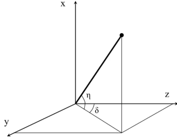
The geometrical parameters involved in the PF model (Figure 2.10(a)) are the components of the unit vectors n1 and n2 of the hinge rotation axis expressed re-spectively in Sf andSp, the coordinates of the position vectors Q1 and Q2 of the intersections of the same axis with the x-y reference planes expressed respec-tively inSf andSp, the coordinates of the insertion points C1 and D1expressed respectively inSt andSp, the fixed distance L between C1and D1 and the fixed distance λ between Q1and Q2. Since the norm of the hinge unit vector is unitary, the components of the unit vectors n1and n2can be expressed as a function of two independent coordinates only, for instance the azimuth δ and the altitude η, y-z being the horizontal plane and z-axis the azimuth origin (Figure 2.11):

n1=   sin η1 cos η1sin δ1 cos η1cos δ1  , n₂=   sin η2 cos η2sin δ2 cos η2cos δ2   (2.3)

Furthermore, the coordinates of the position vectors Q1and Q2admit the following representation: Q1=   x₁ y1 0  , Q₂=   x₂ y2 0   (2.4)

From (2.3) and (2.4) and from the previous considerations, it follows that the PF model is described by means of 16 independent geometrical parameters. It is worth

x

y

z

δ η

Figure 2.11: The azimuth δ and the altitude η angles which identify the n1and n2 unit vectors with respect toSf andSp.

noting that the parameters which define the position of points C2and D2 are not taken into account since they are not necessary for the solution of the position analysis problem of the mechanism in passive flexion: since the prismatic joint is idle, the group C2D2does not influence the motion of both the patella and femur.

The set of 16 parameters is used to define the closure equations of the PF model: Rf pn2= n1 Rf pQ2+ Pf p= λ n1+ Q1 Rtf(Rf pD1+ Pf p) + Ptf− C1 = L (2.5)

where k·k is the L2-norm of the vector. The first two vectorial equations force the axis identified by n1and Q1to be coincident with that identified by n2and Q2. Moreover, the second vectorial equation imposes a constant distance between Q1 and Q2. The last scalar equation ensures that the distance between C1 and D1 is constant.

If the relative motion of the femur and tibia is given — i.e. if Rtf and Ptf are known by solving the closure equations (2.2) — (2.5) is a system of seven equa-tions in six unknowns, i.e. the three components of Pf p and the angles α, β , γ which define Rf p. However, in the first vectorial expression of (2.5) only two out of three equations are independent, since n1and n2both have unitary norms. Thus, given Rtf and Ptf, the system (2.5) makes it possible to find the relative poses of the patella and femur at each assigned flexion angle. It is worth noting that if the flexion angle is externally imposed, the PF motion depends from that of TF: this is an anatomical constraint which is satisfied in the model (system (2.5)).

Equations (2.5) and (2.2) are the closure equations of the knee joint in passive motion. They make it possible to find the relative poses of the patella, femur and tibia by assigning the flexion angle. As previously anticipated, points C2 and D2 have no influence on the closure equations of the mechanism in passive flexion. If the prismatic joint displacement s is required, it is sufficient to solve the position analysis problem and then to evaluate the distance between the points C2and D2.

The 16 parameters which define the passive motion model of PF have to be identified in order to complete the first step of the sequential approach. The pro-cedure of identification is described in section 3.2. The structures which guide the passive motion of PF are identified in the knee model as a result: they are not changed during the following steps, in order to observe the first rule of the sequen-tial approach.

The final result of the first step of the proposed procedure is a set of 35+16 parameters which define a model of the passive motion of the whole knee and, at the same time, which constitute the first block of the sequential approach, i.e. the foundations on which the complete model of the knee has to be built. The prelimi-nary model obtained from the first step can reproduce the passive motion only; the next steps of the procedure enrich this model by adding new anatomical structures, making it possible to reproduce the behaviour of the knee even under different loading conditions.

2.4

Second step: the stiffness model

The motions of the knee when static external loads are applied (muscular loads excluded) are considered in the second step of the proposed procedure. These problems are referred to both as quasi-static and as dynamic problems in the liter-ature, in the sense that the motions of the joint are unknown, while the loads are given. They make it possible to identify several parameters connected to the stiff-ness of the passive structures of the knee — also including those not involved in the passive motion. At the same time, since the external loads do not include mus-cular forces, all parameters connected to the muscles must be ignored; moreover, since the loads are static, all parameters connected to time-varying quantities (as the inertia of the masses or the internal damping of the knee structures) must not be considered. These parameters can be identified in a further step of the sequential approach, as required by the first rule of the procedure.

All these considerations suggest to regard the motions produced by external loads as further basic tasks. They indeed meets the requirements of simplicity and relevance, as described in section 2.2.1: they emphasize the role played by a limited number of structures to stabilize the joint under some defined loading conditions; furthermore, they make it possible to ignore the presence of other structures and of other parameters which do not influence the considered motions. These tasks show the restraining capability of the passive knee structures, a fundamental characteris-tics for the restoration of the knee stability.

A further reason which leads to the choice of these motions as the basic tasks for the second step of the procedure is their anatomical and clinical significance. The analysis of the movement of the knee when subjected to external loads is in-deed a common clinical practice to locate eventual damages or ruptures of the pas-sive structures of the knee, since a high mobility of the joint is normally associated to these damages. Among the infinite combinations of external loads, it is thus ad-visable to choose loading conditions that reproduce these clinical tests. These tests indeed have been devised to stress all the passive structures of the knee, and they have been improved by the clinical practice to test and to analyse the stability of the joint. Thus, they are a well-founded reference to model the restraining structures of the knee.

Three out of the most common clinical tests are the drawer, the torsion and the ab/adduction tests. The first consists in applying an anteriorly or posteriorly directed load to the tibia and to analyse its anterior or posterior displacement at several flexion angles: the test has been devised in particular to stress the ACL and PCL, but several studies prove that the posterior structures of the knee also have an important role in restraining anterior-posterior displacements, thus affect-ing the test [12, 20]. The torsion test consists in applyaffect-ing a moment along the tibia longitudinal axis and to determine the internal/external rotation at several flexion angles: this loading condition is particularly useful to test the posterior structures and the collateral ligaments. The ab/adduction test consists in applying a moment to the tibia along its anterior axis in order to obtain an ab/adduction rotation which

is analysed at several flexion angles: this test in particular stresses the collateral ligaments of the knee.

It is worth noting that all these tests — as the passive motion — can be carried out in vivo and, as a consequence, they make it possible to set the model param-eters on a patient. This is a fundamental aspect when the knee model is used as a tool to assist surgical planning or prosthesis setting, as clarified in section 2.2.3. Moreover, this characteristic allows other important applications in the fields of clinical analysis and rehabilitation. The comparison between the results of the clinical tests obtained in vivo from a patient and those obtained from the model could provide significant insights for a correct and more precise diagnosis. In the common practice, these results are indeed qualitatively analysed, in general, and their interpretation is based on clinical experience; on the contrary, a clinical test model is a quantitative tool which could provide more objective and detailed results to identify damages or deficiencies in the passive structures of a patient’s knee.

The drawer, torsion and ab/adduction tests are taken as a reference for the sec-ond step of the proposed procedure: the correspsec-onding relative motions of the tibia, femur and patella are regarded as the basic tasks of this step. They make it possible to identify the stiffness characteristics of the passive structures of the joint. As a consequence, the final result of the second step of the sequential approach is the stiffness model of the knee.

2.4.1 The multi-fibre model

In order to define the stiffness model of the knee, a stiffness model of the passive structures is required. In the literature, several studies have modelled the stiffness characteristic of the knee and, in particular, some authors have defined models which can replicate the relative motion of the femur, tibia and patella during clinical tests. Some of them used 3D finite elements to model the visco-elastic properties of ligaments [2, 18, 23]; other authors used simple elastic line elements [4, 24, 25]. Since a detailed map of stress and strain of ligaments is not within the scopes of this dissertation, the second simpler approach is used instead. This simplified technique already proved to provide an accurate and sufficiently detailed description of the stiffness characteristic of the knee ligaments [5, 24].

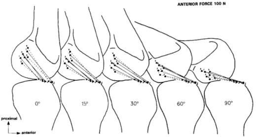
Each ligament is modelled by means of a set of elastic fibres: each fibre in the model replaces a bundle of fibres of a ligament. This is why this method is known in the literature as multi-fibre approach (Figure 2.12). Despite the tech-nique used for the stiffness model has already been proposed by other authors, the multi-fibre model presented in this dissertation contains some original contribu-tions. The main difference lies on the definition of the fibres which constitute each ligament: the fibres are chosen on anatomical bases as in [24], but the application of the rules imposed by the sequential approach forces to use particular anatomical fibres also, i.e. the fibres which guide the passive motion. This aspect is clarified in the following. Furthermore, the sequential approach and the passive motion model which stems from the first step make it possible to originally extend the

ANTERIOR FORCE 100 N

POSTERIOR FORCE 100 N

(b)

proxim

? 4 anterior

Fig. 3. Medial views of the line element representations of the ACL (a) and the PCL (b) in situ at 0. 15,30,60 and 90” of flexion with an anterior and posterior force of lOON, respectively. A loaded line element is presented by a continuous line and a nonloaded line element by a dotted line. The femoral insertion sites of these line elements are presented by square markers and the tibia1 insertion sites by round markers. Legends: Fiber bundles: 1. posterior, 2. posterolateral, 3. posteromedial, 4. central, 5. anterolateral, 6.

anteromedial, 7. anterior.

studies the indirect effects are also included. The method is not limited with respect to the complexity of the knee loading configuration and the degrees of freedom of the test as is the case in dissection studies in which the maintenance of the path of motion before and after dissection of a structure is a prerequisite (Blomstrom

et al., 1993; Takai et al., 1993; Vahey and Draganich, 1991).

However, our approach carries practical limitations. The experimental technique applied is extremely time consuming and technologically involved. Secondly, the ligaments are represented by a number of line elements which do not interact with each other. It was assumed that the effects of mechanical bundle-matrix and inter- bundle interactions are negligible. For the ACL it was demonstrated that longitudinal separation of the

anterior and posterior portions of the ACL influences the stiffness of the knee in anterior tibia1 loading only minim- ally (Blomstrom et al., 1993; Takai et al., 1993). However, it could be a factor which affects the accuracy of our results. Furthermore, it is assumed that the multi-line- element models can extrapolate information to other ligament orientations which occur in situ, but were not represented in the bench tests. Implicitly, it is assumed that the bundles are small enough to assume their force-length relationships independent of the relative ori- entations of the bones. Some of the uncertainties inherent to these limitations, however, have been removed by a global validation study of the ligament models, recently performed in our laboratory (Mommersteeg et al.,

1995a). Of course, these limitations are not inherent to our approach in general, because the multi line element Figure 2.12: The multi-fibre model of a ligament [25].

multi-fibre approach for the modelling of the contacts between the femur and tibia condyles. Finally, the identification procedure based on optimization (section 3.2) shows some differences with respect to other papers in the literature, because of the rules of the proposed procedure (section 2.2).

Each fibre of the multi-fibre model considered in this dissertation is a simple line element which connects its attachments on the tibia and on the femur: fibre-fibre and fibre-fibre-bone interactions are not considered. The force exerted by each fibre-fibre

jof a ligament is:

Fj= kj ε2j εj> 0

Fj= 0 εj≤ 0

(2.6) where kjis a stiffness parameter and εjis the strain of the fibre:

εj=

Lj− L0 j

L_{0 j} (2.7)

in which Lj and L0 j are respectively the length and the zero force length of the fibre, i.e. the limit length which divides tension (first equation of (2.6)) from laxity (second equation of (2.6)) conditions of a fibre. The F-ε relation (2.6) has been chosen among all those proposed in the literature for its simplicity: it is sufficient a single parameter to characterize a fibre; on the contrary, a linear-parabolic or an exponential relation — often used in the literature — requires two parameters [46]. It is worth noting that a fibre can actually intersect another fibre or a bone. The problem could be overcome by using fibre-fibre and fibre-bone contact models. Some simplified contact models have been proposed in the literature [3, 11] which can take into account some fibre-bone interactions; a more accurate model which can take into account also fibre-fibre contact has been recently proposed [7, 40].

These studies prove that fibre-fibre interactions have a limited influence on the model, while fibre-bone contacts can actually affect knee motion. Anyway, fibre contact models are not considered in this dissertation to simplify the knee model and reduce the computations of the identification procedure.

The described multi-fibre model is applied to the principal ligamentous struc-tures of the knee, as reported in Table 2.1. The numbers of fibres of ACL, PCL and MCL are chosen in agreement with [24].

It is worth noting that only the stiffness characteristics of the passive structures of TF has been modelled. Since muscular loads are not considered in this step, the quadriceps and, as a consequence, the PT are not tight: the PF is in passive conditions and the model obtained from step one still holds (section 2.3.2). In particular, the relative motion of the patella and femur can be obtained from the system (2.5). Anyway, the motion is different from that obtained in the first step, since the relative poses of the femur and tibia (described by Rtf and Ptf) are not the same as before: this is in agreement with experimental observations.

The stiffness model of ACL, PCL, MCL includes the IF also (section 2.3.1), which are obtained at the first step of the procedure. At the first step the IF are rigid links that guide the passive motion of TF. At the second step the IF are not rigid and can lengthen by following the F-ε law (2.6); even though they are not isometric any more, these fibres will be referred to as IF in the following, to differentiate them from the others. In order to obey the first rule of the sequential approach, the attachments of IF and their lengths L0 j remain those which have been identified at the first step. As a consequence, only parameters kj have to be identified at the second step, as regards these fibres.

As regards the other fibres, both L0 j and kj parameters must be identified; the attachments are not changed during the identification process to simplify compu-tations. In order to obey the second rule of the sequential approach, L0 jlengths are inferiorly bounded: their minimum values are chosen so that these fibres are never tight in passive flexion. This requirement can be accomplished by choosing Lmin_{0 j} as the maximum distance reached by the fibre attachments in the passive model,

Ligaments NoF Anatomical information

Anterior cruciate(ACL) 5 Two fibres in the anterior bundle, two fibres in the pos-_{terior bundle, one IF.} Posterior cruciate(PCL) 5 Two fibres in the anterior bundle, two fibres in the

pos-terior bundle, one IF.

Medial collateral(MCL) 6 Two fibres in the deeper bundle, three fibres in the su-_{perficial bundle, one IF.} Lateral collateral(LCL) 3 Uniformly distributed fibres.

Posterior structures 5

They include the arcuate ligament (one fibre), the popliteus tendon (two fibres) and the oblique popliteus ligament (two fibres).

during the considered flexion arc: Lmin_{0 j} = max n Tj− R αk tf Sj− P αk tf , αk= αmin, . . . , αmax o (2.8) where Tjand Sj are the tibial and femoral attachments of a fibre, expressed inSt andSf respectively. This requirement guarantees that the passive motion is not influenced by the new fibres, as experimentally proved, and that results obtained at the first step are not modified.

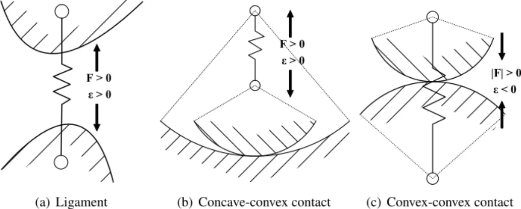
The 5-5 mechanism used for the modelling of TF passive motion makes it pos-sible to extend the multi-fibre approach to model the contact between the condyles. The contact model is indeed similar to that used for the ligamentous structures. The two rigid links that stand for the condylar contacts in the first step are now considered as deformable, in order to take into account the menisci strain and the possible bone separation. The F-ε model (2.6) can be used for medial condylar contact, while it must be slightly modified for lateral contact:

Fj= −kjε2j εj< 0

Fj= 0 εj≥ 0

(2.9)

This is a consequence of the different concavity of the tibial and femoral condyles: the lateral condyles are both convex; the tibia medial condyle is concave, while the femur one is convex. This characteristic affects the relative position of the two attachments of each CF and, as a consequence, the direction of the constraints. A graphic explanation is given in Figure 2.13. The contact model could be refined by substituting the first of (2.9) with a more accurate F-ε law, but this aspect is outside the scope of this dissertation. The insertion points and L0 j lengths of the contact fibres remain those obtained at the first step, in order to satisfy the first rule of the sequential approach; the kjparameters of CF are not identified in this study and are fixed at high values in order to simulate a quasi-rigid contact.

F > 0 ε > 0 (a) Ligament F > 0 ε > 0 (b) Concave-convex contact |F| > 0 ε < 0 (c) Convex-convex contact

Figure 2.13: The relations between strains and forces of ligament (a), medial condyle (b) and lateral condyle (c) fibres of the proposed multi-fibre model.