A model to assess the emission of individual isoprenoids emitted from Italian ecosystems

UNIVERSITÀ DEGLI STUDI DELLA TUSCIA DI VITERBO

AGROALIMENTARI E FORESTALI (DIBAF)

CORSO DI DOTTORATO DI RICERCA

ECOLOGIA FORESTALE

- XXIV Ciclo

A MODEL TO ASSESS THE EMISSION

OF INDIVIDUAL ISOPRENOIDS EMITTED FROM

ITALIAN ECOSYSTEMS

settore scientifico-disciplinare AGR/05

Coordinatore: Prof. Paolo De Angelis Firma ………..

Tutor: Dott. Paolo Ciccioli Firma………

Co-Tutor: Dott. Giorgio Matteucci Firma………

Dottoranda: Claudia Justina Kemper Pacheco

1 Contents

INTRODUCTION 3

OBJECTIVES OF THE STUDY 5

1 BIOSYNTHESIS OF BIOGENIC VOLATILE ORGANIC COMPOUNDS

(BVOC) BY TERRESTRIAL ITALIAN ECOSYSTEM

6

1.1 The plant as a BVOC factory 6

1.2 Molecular and chemical aspects of BVOC synthesis 8

1.3 Storage BVOC and emission process 12

1.3.1 Algorithms utilized 13

1.4 Emission Mechanism 16

2 _{RELEVANCE OF BVOC IN PHOTOCHEMICAL SMOG POLLUTION AND}

GLOBAL CLIMATE CHANGES

19

2.1 _{Global scale} 19

2.2 Lifetime of Isoprene and reactions with OH and O3 19

2.3 _{Formation of aerosols} 23

2.4 The relationship between VOC and Organic Aerosol and VOC and NOx 26

3 _{PROBLEM OF MODELLING} 28

4 EXPERIMENTAL 30

4.1 _{Vegetation Maps} 30

4.1.1 Land cover maps 30

4.2 Meteorological maps 32

4.3 Foliar biomass density 34

4.4 Method utilized for measuring BVOC fluxes 35

4.5 _{Model Run} 35

4.6 Evaluation of model performance 37

5 _{MODEL DEVELOPMENT} 39

5.1 General structure of the model 39

5.2 _{Development of species-specific vegetation maps} 39

5.3 Basal emission rates used in the species-specific model 43

5.4 _{Modification of the short-term emission algorithm, to account for the seasonality}

of isoprenoid emissions

53

5.5 Parameterization of processes 56

5.5.1 Canopy light extinction 57

5.5.2 _{Biomass litter} 58

5.6 Estimate of the species-specific basal emission 59

2

6 RESULTS PROVIDED BY MODEL 61

6.1 Total annual BVOC emissions from Italian forest ecosystems 61

6.2 Distribution of the total isoprenoid emissions among the Italian Regions 62

6.3 Main isoprenoid species emitted by Italian forest ecosystems 64

6.4 _{Monthly trends of isoprenoid emissions and complexity of the emission} 65

6.5 Individual isoprenoids emissions for the July 2006 69

6.6 Model validation 71

6.6.1 Collelongo site 71

6.6.2 _{Castelporziano site} 74

6.7 Comparison with other models 76

7 _{POTENTIAL APPLICATION OF THE MODEL AT THE CHANGE OF}

LAND USE DUE TO DEFORESTATION AND BURNING

77

7.1 _{Land cover changed in burned areas (2000-2006)} 77

7.2 Methodology 77

7.3 Result and Discussion 79

7.4 Changes in the BVOC emissions due to biomass burning 83

8 CONCLUSIONS 85

3

INTRODUCTION

Biogenic volatile organic compounds (BVOC) are organic trace gases other than carbon dioxide and carbon monoxide released from above- and below-ground plant organs.

BVOC emissions can affect directly or indirectly the atmospheric concentrations of air pollutants and greenhouse gases such as ozone and carbon monoxide, as well as the formation of aerosols (Andreae, et al., 1997); (Atkinson, 1990); (Fehsenfeld, et al., 1992); (Graedel, 1979). The term BVOC is used to identify isoprenoids (isoprene, monoterpenes, sequiterpenes and oxygenated terpenes) but also alkanes, alkenes, carbonyls, alcohols, esters, ethers and acids also emitted by plants.

Isoprenoid compound emitted by terrestrial vegetation can be classified mainly into three classes: hemiterpene compounds, such as isoprenene having 5 carbon atoms in the molecule, monoterpenes with 10 carbon atoms in the molecule, and sesquiterpenes with 15 carbon in the molecule. In general, isoprene and monoterpenes are, by far, the most abundant BVOC released by plants (Karl, et al., 2009).

The main factor determining the type and quantity of BVOC emissions in the atmosphere is the distribution of plant species covering the land surface. Within each vegetation type BVOC emission are mainly influenced by the photosynthetically active photon flux density (PPFD) reaching the leaf surface, the leaf temperature and the soil moisture (Karl, et al., 2009). Among these environmental factors, temperature and light are, by far, the principal parameters determining short-term BVOC emissions (Guenther, et al., 2000); (Kesselmeier, et al., 1999). Isoprenoids compounds are emitted from coniferous, deciduous as well as broadleaved evergreen trees as a function of temperature, or both temperature and light (Kesselmeier, et al., 1999).

Once emitted into the atmosphere BVOC react producing tropospheric ozone and other photochemical oxidants in the presence of sufficient amounts of nitrogen oxides (NOx) and UV light (Kanakidou, et al., 2005), oxidation products from several monoterpenes are also known to undergo gas-particle partitioning, and they have been found in atmospheric particles (Yu, et al., 1999); (Kavouras, et al., 1999a). BVOC are generally more reactive than the anthropogenic ones (AVOC): as they react faster with OH radicals to produce ozone, and with ozone to produce secondary organic aerosols (SOA). The atmospheric lifetimes of many isoprenoids range from minutes to few hours (Atkinson, et al., 2003). On a global scale, BVOC emissions from terrestrial vegetation are one order of magnitude higher than those of AVOC) (Guenther, et al., 1995). Although they occur most in tropical areas, they are also important in temperate regions: in many industrialized countries of Europe, BVOC emissions are comparable to AVOC emissions in terms of mass (Friedrich, et al., 1999).

The Italian landscape is characterized by the presence of different forest types, spanning from alpine to semiarid environment, within the Alpine, Continental, Mediterranean and Mediterranean-Temperate climate. The Italian territory shows a strong seasonal variability in the amount of BVOC emissions, mainly related to the high temperature and solar radiation characterizing the summer in the Mediterranean area.

4 So far, national and international emission inventories have been expressed in terms of isoprene and the whole content of monoterpenes. This approach has several limits: the most important one is that the class of monoterpenes is composed by several compounds, the most abundant are about 10-12, of which make up 22% of the total, all displaying different reactivity toward OH radicals and ozone (Atkinson, et al., 2003), and different potentials of SOA productions (Hoffmann, et al., 1997). Indeed, differences in the chemical behavior of monoterpenes are sometimes larger than that between some monoterpenes and isoprene.

While BVOC-specific emission inventories might appear not so important for plant physiologist, they are extremely important for modeling tropospheric ozone and SOA formation. Their estimate is, however, not so easy because it requires a knowledge of the emissions of the different BVOC from the different vegetation species. Furthermore the species specific dependence of isoprenoids emission on biological processes is also required. To get reliable data, the development of plant-specific emission models derived from both laboratory and field observations are needed.

While short term emission responses to temperature or light and temperature- are adequately described by the emission algorithms (Guenther, et al., 1995), seasonality terms were recently introduced to account for changes in the emission caused by phenological variations of plants physiology (Ciccioli, et al., 2003); (Staudt, et al., 2000); (Schnitzler, et al., 1997).

This work presents a novel method to derive BVOC-specific emission inventories starting from vegetation maps. Using laboratory and field data, BVOC-specific maximum emission factors were estimated for the main forest species in Italy. Proper algorithms were developed to predict diurnal and seasonal variations of isoprene and individual monoterpene emissions from these species. BVOC-specific emission maps for 20 vegetation species in Italian ecosystems were obtained by creating an emission model in a GIS environment. The model has been created for the year 2006, with a 1 km x 1 km spatial and 1 h temporal resolutions. Data provided by the model are particularly suitable to be used for the prediction of tropospheric ozone and photochemical oxidants with mathematical models in areas, such as the Italian peninsula, where the large biodiversity leads to complex compositions of BVOC emissions. The model resolution allows to predict photochemical smog pollution at local as well as meso- and global scale. Results are compatible most with Lagrangian models but they can also be used in Eulerian models providing that prediction is made at a mesoscale level.

5 OBJECTIVES OF THE STUDY

The aim of the study is to develop a GIS-based model to estimate the emission of Biogenic Volatile Organic Compounds (BVOC) from forest ecosystems in Italy. The purpose of the model is to generate a species-specific emission inventory for isoprene and individual monoterpenes with validation on experimental data collected in selected sites of the CARBOITALY project.

The work was subdivided in several topics according to the following specific objectives and methodological approaches used for their attainment:

 To develop a detailed and flexible methodology that could be used in conjunction to photochemical models to assess the production of Ozone e secondary organic aerosol (SOA).

 To create updated maps of vegetation to estimate specie-specific BVOC emissions, through the intersection of information from CORINE IV Land Cover maps and from National Forest Inventory (INFC) data.

 To create maps of density of foliar biomass, source of BVOCs, combining the maps previously created with maps of Leaf Area Index (LAI) provided by the CARBOITALY project.

 To generate maps of photosynthetic active radiation (PAR) and leaf temperature considering sunshine hours from daily averages.

 To produce specie-specific maps of daily, monthly and annual emissions of BVOCs for the study case of year 2006.

A further source of information will come from the study of land cover changes in burned areas in Southern Europe, that are potentially relevant for the model assessment of BVOC emissions caused by biomass burning in Italy.

6

1. BIOSYNTHESIS

OF

BIOGENIC

VOLATILE

ORGANIC

COMPOUNDS (BVOC) BY TERRESTRIAL ITALIAN ECOSYSTEM

1.1 The plant as a BVOC factory

Plants are multifaceted chemical factories that produce a multitude of compounds ranging from ethylene and methanol to complex terpenoids and nitrogen containing alkaloids. More than 100,000 chemical products are known to be produced by plants and at least 1700 of these are known to be volatile (Dicke, et al., 2010), as shown schematically in Figure 1-1. Over the earth, terrestrial vegetation is, by far, the most important natural source for BVOC. Their short-term emissions are driven by in temperature or temperature and PAR (Guenther, et al., 1995). Terrestrial vegetation produces and releases a wide spectrum of BVOC, amongst which isoprenoid components (isoprene, monoterpenes and sesquiterpenes) are the most abundant and, very often, the most reactive. In addition to isoprenoids, other VOC (OVOC), such as methanol and carbonyl compounds are produced and released (Winer, et al., 1992); (Kesselmeier, et al., 1997); (Helmig, et al., 1999). Depending on emission quantity and quality, the atmospheric degradation of volatile isoprenoids affects directly or indirectly the atmospheric concentrations of ozone and particulate matter that are important air pollutants and species relevant to earth warming, (Andreae, et al., 1997); (Atkinson, 1990); (Fehsenfeld, et al., 1992); (Graedel, 1979). Global scale emissions of BVOC from terrestrial vegetation are estimated to be in the range of 1.000 Tg C yr-1 (Guenther, et al., 1995), whereas those from man-made activities are calculated to be 150 Tg C yr-1 (Muller, 1992); (Piccot, et al., 1992); (Veldt, et al., 1993); (Steinbrecher, 1994).

7

Figure 1-1 A”VOC tree” illustrates that plants have the metabolic potential to produce and emit a variety of VOCs. In this scheme a hypothetical tree emits all known major plant VOCs plus floral scents. The probable plant tissues and compartments for VOC formation are indicated

BVOCs are released from above- and below-ground plant organs. In general, flowers and fruits release the widest variety of BVOCs, with emission rates peaking at maturation (Dixon, et al., 2000); (Knudsen, et al., 2006); (Knudsen, et al., 2006); (Soares, et al., 2007). Leaves represent the most important BVOC sources in terrestrial plants. The vegetative parts of woody plants are more likely to release diverse mixtures of terpenoids, including isoprene, monoterpenes, sesquiterpenes and some diterpenes (Owen, et al., 2001); (Keeling, et al., 2006), whereas grass species emit relatively large amounts of oxygenated BVOCs and some monoterpenes (Kirstine, et al., 1998); (Fukui, et al., 2000).

chloroplasts (?) HERMITERPENES + MONOTERPENES ISOPRENE 2-METHYL-3-BUTEN-2-OL resin ducts or glands STORED MONOTERPENES MONOTERPENES

leaves, stems, roots OTHER C1– C3 METABOLITES FORMALDEHYDE FORMIC ACID ACETALDEHYDE ACETIC ACID ETHANOL ACETONE cell walls PECTIN DEPOSITION METHANOL (?) flowers FLORAL SCENTS 100s of VOC cell membranes FATTY ACID PEROXIDATION C6ALDHEYDES C6ALCOHOLS many tissues PHYTOHORMONES ETHYLENE

8

1.2 Molecular and chemical aspects of BVOC synthesis

Little is known about the regulation of BVOC synthesis rates, with probably more than 90% of the genes involved in their biosynthesis still unidentified (Laothawornkitkul, et al., 2009). Terpenes have many volatile representatives. Monoterpenes and isoprene belong to the biochemical class of isoprenoids (or terpenoids), whose carbon skeletons are composed of characteristic C5 units (McGarvey, et al., 1995). According to the

number of C5 units, they are subdivided into hemiterpenes (C5, e.g., isoprene, prenylresidue of cytokinene),

monoterpenes (C10, e.g., sabinene, a-pinene, limonene) and sesquiterpene (C15, e.g., b-caryophyllene,

abscisic acid). Table 1-1 reports some of the most common isoprenoids found in plant emission together the chemical formula, chemical structure, molecular weight and boiling point (Winer, et al., 1992).

Table 1-1 Common isoprenoids detected in terrestrial vegetation emission vegetation. (Fuentes, et al., 2000).

Compound name

Chemical

formula

Molecular

weight

(g mol

)

Boiling

point

(K)

Chemical

structure

Isoprene

C

H

68.12

307

Camphene

C

H

136.24

320

3-Carene

C

H

136.24

441

α-Pinene

C

H

136.24

428

β-Pinene

C

H

136.24

436

Limonene

C

H

136.24

448

Myrcene

C

H

136.24

440

Terpinolene

C

H

136.24

459

Sabinene

C

H

136.24

437

β-Caryophyllene

C

H

204.35

396

α-Humulene

C

H

204.35

396

9

Methyl chavicol

148.20

489

Linalool

C

H

O

154.25

469

Methyl jasmonate

224.30

383

γ-Terpinene

C

H

136.24

455

α-Terpinene

C

H

136.24

447

β-Phellandrene

C

H

136.24

446

α- Phellandrene

C

H

136.24

447

p-Cymene

134.22

450

c- β-Ocimene

136.24

373

t- β-Ocimene

136.24

373

α-Copaene

204.36

397

α-Cedrene

204.36

534

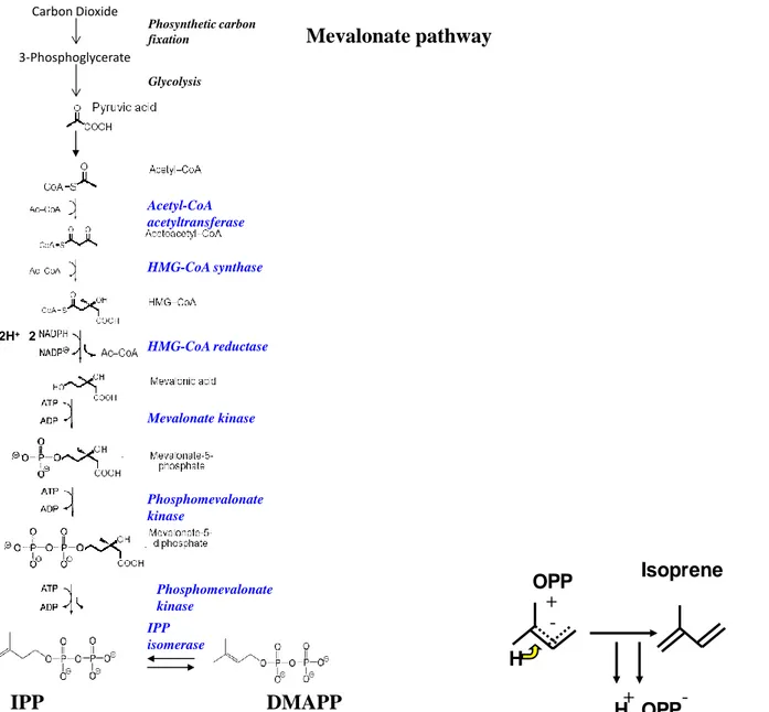
There are two pathways for which you get to the synthesis of isoprenoids in plants, and they are shown in Figures 2-1 and 3-1. Both pathways require phosphorylation energy (ATP), reduction power (NADPH, NADH) and a carbon substrate like pyruvate, glyceraldehydes 3-phosphate, or acetate to form isopentenyl pyrophosphate (IPP) and dimethylallyl pyrophosphate (DMAPP) that are the isoprene precursors. One of the pathways is the so-called DXP pathway, the other the classic Mevalonate pathway. Synthesis of isoprene from IPP and DMAPP requires a specific enzyme, called isoprene synthase.

Today it is believed that most of the isoprene formation occurs in the chloroplast through the DXP pathway, and the formation through the mevalonate pathway is smaller and it occurs most in the cytosol.

10

Figure 2-1 Biosynthetic pathway for isoprene production plants and Isoprene synthase. In the last step in isoprene synthesis is catalyzed by the enzyme isoprene synthase.

Mevalonate pathway

IPP

DMAPP

H

OPP

+

-H

OPP

+

-Isoprene

H OPP

+

-11

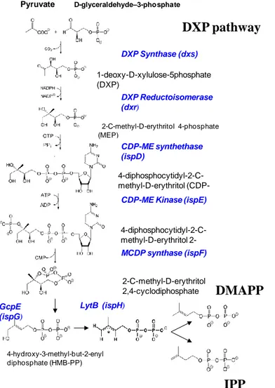
Figure 3-1 Schematic of the DXP pathway of biogenic volatile organic compound (BVOC) biosynthesis in plants.

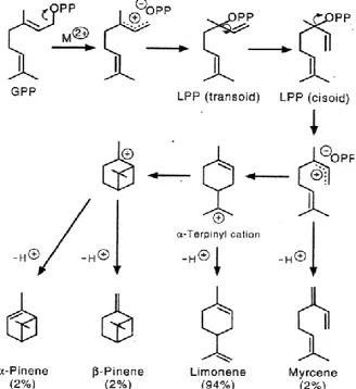
Terpenes and sesquiterpenes are formed by a mechanism similar to that of isoprene, but a preliminary synthesis of geranyl pyrophosphate (GPP) and farnesyl pyrophosphate (FPP) is required. The final compounds are formed by proper enzymes either cyclases or synthases. Figure 4-1 shows the steps for the formation of some monoterpenes through limonene synthase.

DXP Synthase (dxs) D-glyceraldehyde–3-phosphate (GA-3-P) Pyruvate 1-deoxy-D-xylulose-5phosphate (DXP) DXP Reductoisomerase (dxr) 22-C-methyl-D-erythritol 4-phosphate (MEP) CDP-ME synthethase (ispD) 4-diphosphocytidyl-2-C-methyl-D-erythritol (CDP-ME) 4-diphosphocytidyl-C-methyl-D-erythritol 2-phosphate (CDP-ME2P) CDP-ME Kinase (ispE)

2-C-methyl-D-erythritol 2,4-cyclodiphosphate (MCDP) MCDP synthase (ispF) 4-hydroxy-3-methyl-but-2-enyl diphosphate (HMB-PP) GcpE (ispG) LytB (ispH) IPP

IPP

DMAPP

DXP pathway

12

Figure 4-1 Production of terpenes from GPP as performed by limonene.

The scheme was obtained from a limonene synthase isolated from glandular trichomes of peppermint. The steps involves first isomerisation of GPP to linalyl diphosphate (LPP and than cyclization to limonene via a carbocation intermediate (α-terpinyl cation). In the active site of the enzyme, various other carbocation intermediates can form, and proton abstraction from each leads to release of small amounts of myrcene, α-pinene, and β-pinene from (McGarvey, et al., 1995). Similarly to isoprene, the synthesis of monoterpenes occurs most inside chloroplasts, although a minor contribution comes from reactions in the cytosol. There is still a debate about the site where the bulk of sesquiterpnes is produced.

1.3 Storage BVOC and emission process

Isoprenoids produced in the chloroplasts and cytosol may escape through the air passing through the stomata or they can accumulate in storage organs located inside (resin ducts) or outside the plant (glandular trichomas). In the latter case emission occurs much later after the synthesis because compounds need to across strong cellular barrier before they reach the stomatal chamber or the atmosphere. The rate determining step for the emission is diffusion through membranes which is a process solely dependent from temperature (Tingey, et al., 1990); (Guenther, et al., 1995). If synthesized isoprenoids are not stored in specialized organs, their emission occurs few minutes after their formation in the chloroplasts and cytosol. The emission is thus strictly related to the photosynthesis, and is dependent from the light and temperature. Temperature increases the emission because the activity of the enzymes for the production of isoprenoid and their precursors increases exponentially with the temperature according to the well known Arrhenius equation.

13 1.3.1 Algorithms utilized

This different emission behaviour of isoprenoids has been has been formalized into different empirical equations called short-term emission algorithm.

For the light and temperature dependent emission of isoprene, the following algorithm has been proposed and validated by (Guenther, 1997) in many isoprene emitting plants.

(1-1)

The equation allows to predict the emission E° knowledge of the value of the basal emission (E°L+T)

measured at light saturation conditions (1000 µmol gDW-1

h-1) and a standard temperature of 30°C.

(2-1) and (3-1) where α 0.0027, CL1=1.066, CT1=95.000 J mol -1 , CT2=230.000 J mol -1 , CT3=0.961, L= PAR (µmol m -2 s-1), T=Leaf temperature (°K), TM=314 °K, TS=303 °K).

14

Figura 5-1 Behavior of CT and CL for algorithm “L+T” (adimensional) (modificated by Parra et al. (2004)

Figure 5-1 shows that CT is almost zero for a temperature of O°C and exponentially increases with

temperature up to a value of 1,9 at 40°C. For higher temperatures the value of this term decreases quite rapidly. The exponential part of the CT is defined by the increase in the catalytic activity of the isoprene

synthesis with the temperature, as it follows the classical Arrhenius trend. The decline above a certain temperature indicates that the enzyme starts to denaturants. CL increases with an asymptotic trend and

reaches a value of reach 1,1 at 1000 µmol m-2 s-1. The trend of this term is analogous to that of the photosynthesis. In the algorithm both CT and CL are 1 in standard conditions.

In recent years, it has been found that this algorithm is also suitable to describe the emission of monoterpenes from some evergreen and deciduous plants, such as Quercus ilex (Ciccioli, et al., 1997), Fagus sylvatica (Dindorf, et al., 2005), Quercus suber (Pio, et al., 2005) and some tropical plants (Kuhn, et al., 2004). It appears to be suitable to describe the emission of all isoprenoids from the pool directly related to the photosynthesis (L+T pool).

In the case of plants that store mono and sesquiterpenes in specialized organs (resin ducts or glandular trycoma) the emission is decoupled from the photosynthesis and the process driving the emission is diffusion through the organ membranes. The process is only dependent on temperature and only the term CT is

considered. It is generally described by the following equation:

(4-1)

where β , which is the diffusion term, is a term ranging between 0,07 and 0,9, although (Guenther, 1997) has proposed the use on an value of 0,09.

15

Figure 6-1 Behavior of CT for algorithm “T” (adimensional) (modificated by (Parra, et al., 2004)

For monoterpene with dependence on temperature only (MTpool), CT is almost zero for an leaf temperature

of 0°C, increased until almost 2.5 at 40°C and keeps rising for higher temperatures (Figure 6-1).

These algorithms can be successfully applied if the value of the basal is known. One important problem is that the value of this parameter has been found to change through the year and empirical correction terms need to be used to estimate the monthly value of E°, starting from the maximum value measured in the year. Results obtained by various authors have shown that seasonal variations of E° occurs in evergreen oak species (Ciccioli, et al., 2003) and conifers (Staudt, et al., 2000) as well as in broadleaf trees (Schnitzler, et al., 1997). (Ciccioli, et al., 2003) have shown that the seasonality trend of the basal emission is the same as that followed by the photosynthesis, and it seems to be related to real changes in the physiological conditions caused by the natural cycle followed by the plants, due to environmental conditions as well as phenological processes of leaves. (Schnitzler, et al., 1997) has shown that changes in E° are related to the the production and activity of the synthases in leaves.

Another important aspect to consider, is that in some plants both pools can be active, so we may have vegetation species emitting isoprene in the L+T mode and monoterpenes in the T and L+T mode. This is the case, for instance, of Picea abies Karst (Grabmer, et al., 2006).

Measurements of isoprene emissions from Quercus virginiana (Tingey, et al., 1981), Populus tremuloides (Monson, et al., 1989), Eucalyptus globulus (Guenther, et al., 1991); Populus tremuloides, Quercus alba, Populus fremonlii (Fall, et al., 1992) and Pueraria lobata (Sharkey, et al., 1993) besides monoterpene emissions from Eucalyptus globulus (Guenther, et al., 1991), Quercus ilex (Loreto, et al., 1996), Picea abies (Steinbrecher, 1989); (Staudt, 1997) and Pinus pinea (Staudt, 1997) showed no significant influence of stomatal conductance on emission rate. Investigations on the localization of isoprene release from single leaves, discerning the abaxial from the adaxial surface by the use of microcuvettes (Quercus virginiana, Platanus occidentalis, (Tingey, et al., 1981); Quercus rubra, (Loreto, et al., 1990); Eucalyptus globules,

16 (Guenther, et al., 1991); Populus tremuloides, Quercus alba, Populus fremonlii, (Fall, et al., 1992), clearly showed that a significant isoprene emission rate was only detectable on that leaf side containing the stomatal pores.

For monoterpene emissions, similar experiments were reported for two plant species only by (Loreto, et al., 1996) founding a monoterpene emission only from the abaxial side of Quercus ilex leaves, whereas (Guenther, et al., 1991) reported emissions from the adaxial side of Eucalyptus leaves. The apparent non-dependence of stomatal closure and isoprenoid emissions has been explained by the low, unsaturated VOC concentrations in the intercellular air spaces of the leaf mesophyll, which increase when stomata close. The decrease in stomatal conductance would, hence, be compensated by an increase in the concentration gradient between in- and outside the leaf (Monson, et al., 1991); (Sharkey, et al., 1991); (Fall, et al., 1992); (Bertin, et al., 1996); (Sharkey, et al., 1996); (Staudt, 1997).

Monoterpenes are potentially able to permeate through the cuticles, as showed by (Schmid, et al., 1992); (Schmid, et al., 1991) and (Estell, et al., 1994), as well as other gases such as CO2, SO2, and O2 having a 2-3

fold higher permeability than water (Schonherr, 1982); (Lendzian, 1987). Moreover, evidence exists that monoterpene emissions from leaves are strongly influenced by cuticula hydratation (Croteau, 1977); (Lamb, et al., 1985); (Staudt, 1997). However, the results obtained with isoprenoids should not be transferred to all trace gas species. In a recent study on Populus sp., (Guidolotti, et al., 2011) found an inverse correlation between isoprene emission and intercellular CO2 concentration and a positive correlation between isoprene

emission and instantaneous water use efficiency. This could indicate an indirect stomatal control on isoprene emission, mediated by a constitutively reduced intercellular CO2 concentration.

1.4 Emission Mechanism

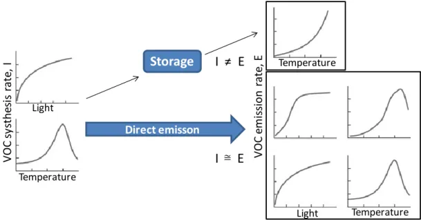
The BVOC emissions from leaves are not only limited by physiological factors, but also by physico-chemical constrains caused by temperature, stomatal conductance and leaf structure (Niinemets, et al., 2004). Therefore, physico-chemical characteristics such as low volatility or diffusion can also control the emission, interacting with physiological limitations. Among the most important physicochemical features, we may mention: i) volatility, determined by gas phase partial pressure, and aqueous and lipid phase concentrations; ii) the diffusion through the gas, aqueous and lipid phases within the leaves and iii) the diffusion from the leaf surface. According to (Grote, et al., 2008), the capacity for compound storage inside the plants, is depending on the control of emissions by differently, shared physiological and physic-chemical factors (Figura 7-1). In species with large storage pools such as conifers, the synthesis (I) and emission (E) rates could be effectively decoupled (I Instead when a storage pools is small, as in the case of isoprene, the synthesis and emission rates are essentially equal (I = E).

Gas phase diffusion at the leaf-air interface, determined by stomatal conductance, can influence significantly the synthesis and the emission of BVOCs with low Henry’s law constants, such as formic acid, formaldehyde and methanol that primarily partition to the aqueous phase (Laothawornkitkul, et al., 2009). This does not apply to the less water-soluble compounds, such as isoprene and non-oxygenated terpenes that

17 partition mainly to the gas phase (Niinemets, et al., 2004), with emission rates generally independent of stomatal conductance. The isoprene, for example, is not stored at all and is highly volatile with a small storage capacity within the leaves: therefore, its emission rate only depends on temperature and light (Laothawornkitkul, et al., 2009).

Figure 7-1 Schematic about the relationship between light and temperature controls of BVOC synthesis rates (I), and light and temperature controls of BVOC emission rates (E) (Grote, et al., 2008).

(Guenther, et al., 2000) investigated on the different mechanisms that regulate the BVOC emission from vegetation. Two of these processes have been described: (a) Synthesis in Chloroplasts and (b) Defense in specialized tissues. In the latter case, the algorithm to derive emission activity is an exponential increase with the temperature such that proposed by Guenther and colleagues (Guenther, et al., 1993), previously shown (see section 1.3). The processes occuring in chloroplasts, including emissions of isoprene (Guenther, et al., 1993), 2-methyl-3-buten-2-ol (MBO) (Harley, et al., 1998) and some monoterpenes (Kesselmeier, et al., 1996); (Ciccioli, et al., 1997), can be described as the product of temperature and the light (photosynthetic photon flux density (PPFD) (Guenther, et al., 1993). Such environmental responses were included in empirical emission algorithms that predicted plant emissions with high predictive power in some, but not in all, situations (Guenther, et al., 2000).

Until recently, it was believed that monoterpenes were emitted only by conifers and their release controlled by the needle temperature. All other vegetation species were believed to emit isoprene with a mechanism that was dependent on light and leaf temperature (Fall, 1999). Recent studies performed on European evergreen oaks (Ciccioli, et al., 1997); (Pio, et al., 2005) and deciduous species of Europe (Dindorf, et al., 2006) as well as Amazonia (Kuhn, et al., 2002) have clearly shown that both evergreen and deciduous species can emit monoterpenes with the same light and temperature dependent mechanism followed by isoprene-emitting plant. Other studies have also shown that not all conifers emit monoterpenes in a temperature-dependent

V O C e m is si on rate , E Temperature Temperature Light V O C s ys the si s rate , I Light Temperature

Storage

I ≠ E

I E

18 mode. Some conifers (such as spruce), myrtle and eucalyptus that are common in Europe emit isoprene and monoterpenes in light and temperature dependent way (Grabmer, et al., 2006); (Staudt, et al., 2000); (Kesselmeier, et al., 1999).

The Mediterranean area includes a large number of forest ecosystems, and most of these produce and release large amounts and mixtures of terpenoids. Some species, such as Quercus ilex L. release terpenes directly after their synthesis (Staudt, et al., 2001). Instead, others store these biogenic volatile organic compounds prior to release, like Pinus halepensis Mill. (Llusià, et al., 2000).

The above studies of Quercus ilex demonstrated that the production and release of high amounts of monoterpenes by plants are not necessarily restricted to species storing essential oils in glandular organs. Moreover, oak forests can also constitute an important source not only of isoprene but also of monoterpenes. Nevertheless, not all oaks are isoprene emitters, with Quercus cerris that is a negligible emitter (Steinbrecher, et al., 1997).

According to (Niinemets, et al., 2002), monoterpene emissions respond to environmental modifications, but the emissions do not respond instantly to changes in the synthesis rates because of low volatility and low diffusion within the leaves.

In general, all studies on the emission of isoprene and monoterpenes show clear temperature dependence. Additionally, isoprene emissions have been shown to be triggered by light, as a result of the link between isoprene emission and synthesis from photosynthetic products. As no large isoprene pool exists, synthesis and hence emission will cease within minutes under dark conditions (Ciccioli, et al., 2003); (Evans, et al., 1985); (Guenther, et al., 1991); (Kesselmeier, et al., 1999); (Monson, et al., 1991); (Sanadze, 1991); (Sharkey, et al., 1991); (Tingey, et al., 1981).

19

2. RELEVANCE OF BVOC IN PHOTOCHEMICAL SMOG POLLUTION

AND GLOBAL CLIMATE CHANGES

2.1 Global scale

Emissions inventories are based on emission factors, data on climate, land use, and/or vegetation types as well as biomass distribution. The emission factor specifies the basic emission or emission capacity of a plant species under standard conditions, usually at a temperature of 30°C and a photosynthetically active radiation (PPFD) of 1000 µmol photons m-2 s-1. Some models cover specific climatic conditions within the vegetation canopy (Lamb, et al., 1993). Regional and global emission inventories for hydrocarbons include the most important monoterpenes and isoprene (Zimmerman, 1979); (Lamb, et al., 1993); (Graedel, et al., 1993); (Guenther, et al., 1995); (Simpson, et al., 1995). Estimates for the global carbon input by these compounds range between 127 and 480 Tg C yr-1 for monoterpenes and between 175 and 503 Tg C yr-1 (Guenther, et al., 1995) for isoprene: these values are in the same range of methane release (ca. 500 Tg C yr-1, (Crutzen, 1991)) and significantly higher than anthropogenic nonmethane hydrocarbon emissions (ca. 100 Tg C yr-1, (Singh, et al., 1992).

Therefore, the emissions of BVOC far exceed the global anthropogenic VOC. Though many BVOC species have been identified to be emitted from plants, much of the global flux and subsequent effect on atmospheric chemistry is probably caused by a relativity small number of compounds. Isoprene makes the largest contribution, followed by the monoterpene family (Levis, et al., 2003).

Sesquiterpenes are important precursors to secondary organic aerosols (SOAs) (Hoffmann, et al., 1997); (Bonn, et al., 2003), but estimating their emission rate and related compounds is difficult because of their reactivity and low vapour pressures. Furthermore, some oxygenated compounds, such as methanol, acetone and acetaldehyde, can play an important role in the atmosphere chemistry (Guenther, et al., 1995); (Kesselmeier, et al., 1999); (Fuentes, et al., 2000).

2.2 Lifetime of Isoprene and reactions with OH and O

When reactive BVOCs are released into the atmosphere, they are subject to oxidation reactions, potentially leading to the ultimate products of CO2 and water (Laothawornkitkul, et al., 2009).

Many gas-phase oxidation products have been identified from the ozonolysis of terpenes, including low molecular weight compounds, for example formaldehyde, acetone, and formic acid, and higher molecular weight products such as nopinone and pinonaldehyde, as well as other multifunctional compounds with carbonyl, carboxyl or hydroxyl groups (Calogirou, et al., 1999); (Jang, et al., 1999).

The VOC can rapidly react with the hydroxyl radicals (OH) resulting from the UV photolysis of tropospheric ozone (O3) and other photochemical products, such as low molecular weight carbonyls, mentioned above.

The initial products of the VOC-OH reaction can be further oxidized to form peroxyradicals (RO2). This can

20 (a) Hydrogen abstraction to a saturated hydrocarbon

(b) Hydroxyl radical addition to an unsaturated hydrocarbon

Both organic radicals react with oxygen to produce peroxyalkylradicals:

R· + O2 ROO· RO2· HOR· + O2 HOROO· H H H C H H H C H H H C H H H C OH + OH

.

Hydroxyalkyl radical (HOR.₎

H H C H H C OH + OH

21

Figure 1-2 Schematic diagram summarizing of VOC to produce peroxyradicals (RO2·).

In the presence of sufficient oxides of nitrogen, these RO2 species may oxidize NO to NO2, which can, in

turn, be photodissociated, leading to the formation of O3 and the regeneration of OH (Figure 1-2).

Hydroperoxyradicals can also convert NO to NO2 re-introducing OH radicals into the photochemical cycle.

Therefore OH removed by VOC can be eventually regenerated. With low NOx concentrations, RO2·may

react with hydroperoxy radicals (HO2·) to form less reactive peroxides, which may be removed from the

atmosphere by deposition processes which lead to the net consumption of O3 (Fehsenfeld, et al., 1992).

Besides OH, O3 can themselves act as an oxidant for unsaturated BVOCs (Fehsenfeld, et al., 1992). The

addition of O3 to carbon-carbon double bonds leads to the formation of ozonides, which are unstable free

radicals that can form OH and RO2.

At night, when OH concentrations are effectively zero, BVOC oxidation may be driven by reaction with the nitrate radical (NO3) (Wayne, 2000). Because of its rapid reaction with NO and its short lifetime ( 5 s) in

sunlight as a result of photolysis, NO3 concentrations are low during the day but can increase substantially at

night (Figure 2-2). This may lead to the removal of BVOCs that would otherwise be available for daytime O3

formation. However, the reaction rate of NO3 with most BVOCs are quite low (one-fifth of that with OH in

the case of isoprene), and so reaction with OH is normally the dominant route of oxidation.

+O2 NO NO2 O3 O 3p OH. +hn+H2O R. RO2. HC RO. HO2. RCHO +hn

22

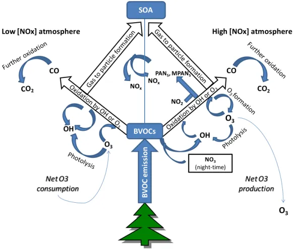
Figure 2-2 Schematic diagram summarizing the current understanding of the roles of biogenic volatile organic compounds (BVOCs) in the chemical components of the Earth system (Laothawornkitkul et al., 2009).

Carbon Monoxide (CO) influences the oxidative capacity of the atmosphere in the same way as isoprene by functioning as a sink for OH (Logan, et al., 1981). Therefore, the oxidation of CO can act as a source or sink of O3, depending on the availability of NOx. Once generated, CO can be transported over large distances

because of its relatively long atmospheric lifetime (several months). BVOCs can therefore, in this way, influence atmospheric chemistry at global scale (Fehsenfeld, et al., 1992); (Lerdau, et al., 1997); (Lerdau, et al., 2002). According to (Calfapietra, et al., 2008), the combination of elevated concentrations of CO2 and O3

resulted in a strong decrease of isoprene emission in open field conditions.

Atmospheric oxidation of BVOCs and their primary oxidation products (e.g. methyl vinyl ketone and methacrolein in the case of isoprene) can, in the presence of NOx, result in the formation of organic nitrates,

including peroxyacetylnitrates (PANs) and peroxymethacrylic nitric anhydrides (MPANs) (Fehsenfeld, et al., 1992). PANs and MPANs have longer atmospheric lifetimes than NOx (days to months) and hence can be

transported over greater distances, allowing them to act as carriers of reactive nitrogen (Figure 2-2).

Several studies evidence that a broad variety of trees emit reactive BVOCs that either do not escape the ecosystem canopy, or are not typically measured by current analytical techniques. (Ciccioli, et al., 1999). Ciccioli and colleagues (1999) argued that terpenes can be oxidized within a forest canopy. These measures were realized within a forest canopy before detection by above-canopy flux techniques in an orange orchard

B V O C e m is si on CO CO2 CO

High [NOx] atmosphere Low [NOx] atmosphere

NO3 (night-time)

O

O

23 in Spain in 1995 and 1996. This species emitted large amounts of b-caryophyllene during the summer. This compound, a reactive sesquiterpene, was observed in leaf enclosures that were not observed in simultaneous above canopy measurements, and suggested they were oxidized before escaping the orchard canopy.

2.3 Formation of aerosols

In recent years biogenic VOCs have been identified as the major precursor substances to the formation of secondary organic aerosols (SOAs) in the atmosphere (Kavauras, et al., 1999b); (Pandis, et al., 1992); (Yu, et al., 1999). The anthropogenic contribution to the SOA formation is small on a global scale, although it can be important in polluted regions (Kanakidou, et al., 2005).

Different laboratory and outdoor chamber experiments, evidence that monoterpenes, isoprenes and sesquiterpenes emitted by vegetation have a high potential to form SOAs, such as also anthropogenic species like aromatic compounds, long-chain alkaenes and alkanes can form SOA (Kroll, et al., 2008); (Surratt, et al., 2006). However, studies over tropical forests have not always found significant SOA production to the expected degree, indicating that further work is needed in this area (Rizzo, et al., 2006).

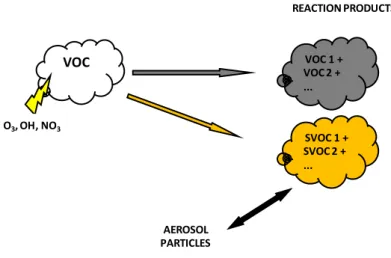
Many details in the formations process of SOA are still unknown, probably by the lack of knowledge of gaseous secondary organics involved in gas/particle partitioning. Kanakidou and colleagues (Kanakidou, et al., 2005) argued that one of chemical mechanism that form SOA is linked to the heterogeneous reactions: this processes result in the decrease of the volatility of the semi-volatile compounds that are partitioned between aerosol and gas phase. Figure 3-2 give an example of SOA formation: VOC are oxidized in the atmosphere mainly by O3, NO3 and OH. The oxidation process adds functional groups to the organic gas

molecules and thus lowers their vapour pressure. This process partly results in gases that are again volatile and do not contribute to the aerosol formation. Another part of the reaction products however might be semi-volatile and condense to form aerosol particle, if ambient conditions are favourable (Dusek, 2000). Thus, SOA formation involves a multiplicity of semi-volatile organic compounds (SVOC) having complex molecular structures. Their low atmospheric concentrations cause analytical difficulties (Jacobson, et al., 2000); (Turpin, et al., 2000); (Kanakidou, et al., 2005). The SVOCs, which evaporate during the emission-dilution process, could condense back to the particulate phase after oxidation. The exact physical and chemical pathways to SOA formation are still not fully understood for most parent hydrocarbons.

Almost all organic material associated with the condensed phase should be regarded as semi-volatile. The SVOCs include any compound with more than 1% of its mass in both the condensed and vapour phases somewhere in the atmosphere. Given the atmospheric range of organic aerosol (OA) mass concentrations of between 0.1 and 100 µg m-3

(Chung, et al., 2002); (Cabada, et al., 2004), compounds with effective saturation concentrations between 0.001 and 10000 µg m-3

should be considered semi-volatile under even the most narrow definition of the term.

24

Figure 3-2 Schematic overview of SOA formation

Although it is known that a substantial fraction of the aerosol particles in remote regions is made of organic material, and that the oxidation of BVOCs may lead to the formation of SOAs, it is not yet clear how important is SOA formation in altering the climate system (Laothawornkitkul, et al., 2009).

Aerosols directly affect climate by scattering solar radiation. They also indirectly alter the arth’s radiative balance by acting as cloud condensation nuclei, changing cloud albedo and the degree of cloud cover, so potentially leading to net cooling of the arth’s surface during the day. Nevertheless increased cloud cover may also reduce the occurrence of low night-time surface temperatures, which can damage plants (Hayden, 1998) or increase average night temperature by reflecting inside infrared radiation.

Isoprene accounts for about half of all natural VOC emission, and several studies detected the presence of humic-like substances (glycol aldehyde, hydroxyl acetone and methyltetrols), indicating the involvement of isoprene as source for SOA (Jang, et al., 2003); (Claeys, et al., 2004a); (Claeys, et al., 2004b); (Limbeck, et al., 2003); (Matsunaga, et al., 2003). Claeys and colleagues (2004b) proposed that a small (0.2%) fraction of all isoprene emissions may be converted into SOA, corresponding to emissions of 2 Tgyr-1.

The VOC potential for SOA formation depends on their lifetime; VOCs such as terpenoid ketones, terpenoid alcohols, and higher olefins, have a lifetime <1 day while less reactive VOC such as methanol and various aldehydes and ketones, have lifetimes longer than 1 day.

According to (Griffin, et al., 1999), only about 30% of the so far described VOC, have the potential to form SOA. In contrast, some monoterpenes and all sesquiterpenes have large potential for SOA formation, because of their high reactivity, with atmospheric lifetime of only a few minutes (see Table 1-2.a,b) (see the square in green) (Hoffmann, et al., 1997); (Jaoui, et al., 2003). According to (Bonn, et al., 2003), the atmospheric new particle formation observed in remote areas and generally attributed to low-volatility oxidation products of monoterpenes, may be actually initiated by products of sesquiterpenes reactions with O3. Other studies, report that carbonyls (>C7) may be important contributors to SOA (Matsunaga, et al.,

2003). Estimates indicate that SOA can be responsible for about 10-40% of the global organic aerosol (OA)

VOC 1 + VOC 2 + ... VOC O3, OH, NO3 SVOC 1 + SVOC 2 + ... AEROSOL PARTICLES REACTION PRODUCTS

25 mass (Kanakidou, et al., 2005); this is the sum of primary organic aerosol (POA) and SOA. In the latter case, about 90% of SOA is currently believed due to biogenic VOCs (Kanakidou, et al., 2005). .

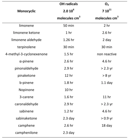
Table 1-2.a Chemical lifetimes of Terpenes and their oxidation products. Data obtained by (Atkinson, et al., 2003).

Monocyclic OH radicals 2.0 106 molecules cm3 O3 7 1011 molecules cm3 limonene 50 min 2 hr limonene ketone 1 hr 2.6 hr

limonene aldehyde 1.26 hr 2 day

terpinolene 30 min 30 min

4-methyl-3-cyclonexenone 1.5 hr non reactive

α-pinene 2.6 hr 4.6 hr pinonaldehyde 2.9 hr > 2.3 yr pinaketone 12 hr > 8 yr b-pinene 1.8 hr 1.1 day Nopinone 10 hr 3-carene 1.6 hr 11 hr caronaldehyde 2.9 hr > 2.3 yr sabinene 1.2 hr 4.6 hr sabinaketone 2.3 day > 0.9 yr camphene 2.6 hr 18 day camphenilone 2.3 day

26

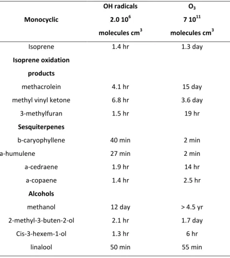
Table 1-2.b Chemical Lifetimes of other biogenic compounds than monoterpenes and their oxidation products. Data obtained by (Atkinson, et al., 2003).

Monocyclic OH radicals 2.0 106 molecules cm3 O3 7 1011 molecules cm3 Isoprene 1.4 hr 1.3 day Isoprene oxidation products methacrolein 4.1 hr 15 day

methyl vinyl ketone 6.8 hr 3.6 day

3-methylfuran 1.5 hr 19 hr

Sesquiterpenes

b-caryophyllene 40 min 2 min

a-humulene 27 min 2 min

a-cedraene 1.9 hr 14 hr a-copaene 1.4 hr 2.5 hr Alcohols methanol 12 day > 4.5 yr 2-methyl-3-buten-2-ol 2.1 hr 1.7 day Cis-3-hexem-1-ol 1.3 hr 6 hr

linalool 50 min 55 min

Table 1-2.a shows as most of the VOCs emitted from biogenic sources are highly reactive in the troposphere, with calculated lifetimes of few hours or less. Moreover some sesquiterpenes, such as b-caryophyllene and a-humulene, can shows an even shorter lifetime in presence of O3 (Table 1-2.b), and they are therefore rapidly removed by oxidation reaction once emitted from vegetation, leading to very low concentrations in the atmosphere (Atkinson, et al., 2003).

2.4 The relationship between VOC and Organic Aerosol and VOC and NO

The ratio of VOC to NOx is one of the most important parameters in the behaviour of the VOC-NOx-O3

system. Moreover, it has a major effect on how reductions in VOC and NOx affect ozone concentrations

(Committee on Tropspheric Ozone, National Research Council (CGER), 1991).

The availability of VOCs and NOx in the morning along with their different reaction rates with the OH

radical can greatly influence how much ozone is formed on a given site in a day (Seinfeld, et al., 1998). The evaluation of the potential for photochemical ozone production of a BVOC compound has to be made for different VOC and NOx concentrations because the production of ozone and photooxidants is strongly

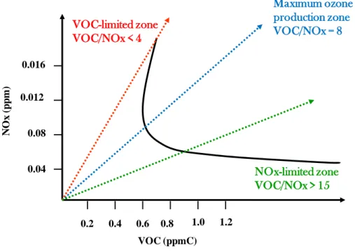
27 The O3 – NOx –VOC connection can be illustrated by a plot (Figure 4-2) generated applying to VOC and

NOx concentrations a basic ozone model called “ mpirical Kinetic Modeling Approach” ( KMA)

(Finnlayson-Pitts, et al., 1999). This graph shows peak of ozone formation as a function of the ratio of VOC to NOx concentrations. It identifies threes regimes with different O3 – NOx –VOC sensitivities. The straight

line in the centre of Figure 4-2, represents a constant VOC/NOx = 8. The values between 5 and 15 are

considered transitional, with an “optimal” production of O3 is estimated in correspondence of VOC/NOx

ratio around 8 (Derwent, et al., 1996).

Figura 4-2 Ozone formation in three different zones of the plot as a function of the VOC/NOX ratio.

In the urban area, (see the dotted line in red), is observed a typical situation of strong polluted areas, characterized by a low VOC/NOx ratio, where NOx emissions have much greater influence, the ozone

synthesis is limited by VOCs concentration.

Instead for the dotted line in green, there is observed a typical situation of low polluted areas (rural). Therefore, we find a NOx sensitive regime for ozone production, because of the higher production of

biogenic VOC with respect to NOx. In this way, in the rural air masses the ozone concentrations are most

efficiently lowered by reducing NOx, shifting in this way the VOC/NOx ratio to less favourable value for

ozone production (The VOC/NOx ratio for maximum ozone production), while in the urban ones the same

goal can be achieved by reducing the VOC concentration.

Moreover, in blue we can see the maximum ozone production zone, while the continue line in black shown a typical trend observed in suburban sites located downwind, such as an urban plume.

Maximum ozone production zone VOC/NOx = 8 NOx-limited zone VOC/NOx > 15 VOC (ppmC) N O x (p p m) 0.04 0.08 0.012 0.016 0.2 0.4 0.6 0.8 1.0 1.2 VOC-limited zone VOC/NOx < 4

28

3. PROBLEM OF MODELLING

An important application of air quality models is to determine how pollutant concentrations respond to changes in emissions. For this type of applications, accurate emission inputs are pivotal to good model performance. Emissions inputs are developed to be compatible with both the chemical mechanism used in the photochemical models, and the model resolution (Russell, et al., 2000). Detailed and speciated VOC emissions should be lumped into the appropriate chemical mechanism categories. Emissions estimates (or inventories) need to be processed into a form used by air quality models via emissions processors that are part of the air quality modelling system.

It is generally believed that emissions are one of, if not the most, uncertain inputs into air quality models, and certainly one of the most important. Biogenic emissions are believed to be very uncertain as well, with scientists often suggesting an uncertainty of a factor of three or more (e.g. (Simpson, et al., 1995)). A recent study, found that the uncertainty in the regionally averaged impact of BVOC on ozone build-up in Europe is estimated to be ± 50%. Evaluating the impact of biogenic VOCs on atmospheric chemistry is subject at least to three types of major uncertainties: emission inventory, modelling of chemical pathways, and ambient NOx

abundance (Curci, et al., 2009).

Biogenic emissions uncertainty appears to be the dominant limitation in the current ability to accurately predict the dynamics of ozone over urban and regional scales, as well as for the impact of control strategies. Although trends in BVOC emission rates as the arth’s climate changes are still uncertain, reactive BVOCs are of obvious concern, as they may give rise to species-specific feedbacks between plants and the atmosphere (Shallcross, et al., 2000); (Fuentes, et al., 2001); (Lerdau, 2007); (Arneth, et al., 2008). Simplistically, it may be expected that climate warming will increase BVOC emissions due to their strong temperature dependence, and so it will increase their atmospheric concentrations, causing a decrease in the concentration of OH, and so leading to a reduction in the capacity of the atmosphere to remove tropospheric methane and CO, resulting in even further global warming. Enhancement of isoprene emissions in response to rising temperatures may also have the dual effect of promoting tropospheric O3 production in NOx

-polluted air, whilst contributing to reduced O3 damage of leaves from isoprene-emitting species (Loreto, et

al., 2001b); (Velikova, et al., 2005).

However, such simplistic models require considerable elaboration, as many BVOCs serve to protect plants against biotic stress such as insect attacks (Miller, et al., 2005); (Poecke, et al., 2004) and because of their role in enhancing plant abiotic stress resistence as well, such as against heat stress and oxidative stress generated by ozone exposure (Affek, et al., 2002); (Loreto, et al., 2001b); (Penuelas, et al., 2005); (Sharkey, et al., 2001); (Sharkey, 2005); (Velikova, et al., 2005). Greater stress resistance induced by BVOC emissions can be of particular significance in a globally changing environment that is characterized by amplification of many abiotic stresses.

Present models are unable to adequately predict these possible interactions and feedbacks, partly because the combined effect of global warming with other global environmental drivers on BVOC emissions may not

29 always give straightforward outcomes. For example, drought episodes may remove the positive effect of warming on isoprene emissions (Fortunati, et al., 2008), whereas enhanced UVB radiation, together with warming, may actually increase emissions (Tiiva, et al., 2007). In addition, changes in cloudiness driven by BVOC emissions and subsequent SOA formation could change the intensity of the impact of photosynthetically active radiations, hence changing the emission rates of some light-dependent BVOCs.

30

4. EXPERIMENTAL

The research carried out over the last years within the framework of the European projects BEMA (Biogenic Emissions in the Mediterranean Area) (Seufert, et al., 1997), BIPHOREP (Biogenic VOC emissions and PHOtochemistry in the boreal regions of Europe) (Laurila, 1999), ECOVOC and VOCAMOD, have shown that many plants present in Southern and Central Europe exhibit an emission behaviour different from plants of the same family growing in North America. In particular, some Mediterranean species are strong monoterpene emitters, but they release them with the mechanism followed by isoprene emitting plant species. Moreover, some common deciduous species are basically non-BVOC emitters. Moreover, the emission-factors of many Mediterranean species are still affected by large uncertainties in terms of emission rates and iosoprenoid composition, and their dependence from environmental factors is still unknown. Emission variations can be induced by differences in latitude, climate and soil type. For some oaks, the tendency to form hybrid may change the emission behaviour. A reliable model for predicting the BVOC emission over the Italian territory requires that all the various parameters influencing the plant emission are taken into a due account. Given the complexity of plant physiology, parameterization procedures were developed in this work to describe as better as possible the effect produced by environmental factors and physiological and phonological processes. Due to the large biodiversity of the Italian forest ecosystems, different parameterization procedures were adopted for the different plant species. The estimate was also complicated by the fact that values of some environmental factors to predict the emission were required at the same spatial and temporal resolution requested by the model.

In this section we summarize the approaches that were developed and adopted to build up the BVOC emission model needed to predict the emission of isoprene and individual monoterpenes from the Italian forest ecosystems at a high spatial (1km x1km) and temporal resolution (daily basis).

4.1 Vegetation maps

4.1.1 Land cover maps

The digital land use map produced by the CORINE IV Land Cover (CLC) for the year 2006 was used in this study. The map, provided by the partners of the CARBOITALY Project, covers 301,330 km2 with a spatial resolution (grid cell size) of 1 km2. The UTM coordinates (North West corner) are the following: X (longitude) = 313,000 m, Y (latitude) = 5,230,000 m. Based on the coverage, the following classes and sub-classes were selected in this study.

2.2 Permanent Culture Subdived into:

31 2.2.3 Olive grove 2.2.4 Wood arboriculture Subdived into: 2.2.4.1 Poplar culture 2.2.4.3 Eucalyptus

3.1.1 Forest areas covered by broadleaf species Subdived into:

3.1.1.1 Forest areas covered by evergreen oaks and evergreen broadleaf species (mainly Q. ilex, Q. suber, Q. cocifera)

3.1.1.2 Forest covered by deciduous oaks (mainly Q. cerris, Q. pubescens, Q. frainetto, Q. petraea, Q. robur)

3.1.1.3 Mixed forest areas covered by autoctonous broadleaf species (Acer platanoides, Fraxinus excelsior, Fraxinus ornus, Ostrya Carpinifolia)

3.1.1.4 Forest area covered by Castanea sativa 3.1.1.5 Forest areas covered by Fagus sylvatica

3.1.1.6 Wooden areas covered by hygrophillic plants (Salix sp., Populus sp., Alnus sp.)

3.1.1.7 Wooden areas covered by exotic broadleaf trees (Robinia pseudoacacia, Ailanthus altissima)

3.1.2 Forest areas covered by conifers Subdived in:

3.1.2.1 Forest covered Mediterranean pines and Cypress trees (P. Pinea, P. Pinaster, P. Halepensis) 3.1.2.2 Mixed forest covered by Mountain pines (P. Nigra, P. Sylvestris)

3.1.2.3. Forest covered by Norway spruce (Abies alba, Picea abies) 3.1.2.4 Mixed forest covered by Larix decidua and Pinus Cembra

3.1.2.5 Forest areas covered by exotic conifers (Pseudotsuga menziesi, P. Radiate, P. Strobes)

According to these maps, the surface covered by deciduous, coniferous and broad leaf forests was 18.20%, 5.09% and 1.09% of the entire territory. Values of the coverage were also provided for each of the subclasses.

These maps, although useful for many forest applications, were not so suitable for estimating species-specific BVOC emission because in many instances, they included forest species exhibiting different emissions and followed different emission algorithms.

The maps, that were originally supplied in the IDRISI format (IDRISI Kilimanjaro, ©Clark Labs, 2006) were converted into an ArcGIS 9.3 (©ESRI, 2008) format, that was used for the model development.

32

4.2 Meteorological maps

Meteorological data on leaf temperature (in K°) and solar surface radiation (W m-2) from MODIS are the drivers used as input for the BVOC emissions model. The meteorological parameters necessary for estimating the BVOC emissions were the foliar temperature and the PAR. Foliar temperature and solar radiation data were provided in grid format maps by CARBOITALY project, at the spatial resolution of 1 km x 1 km and daily temporal resolution for the year 2006. The PAR was therefore not directly available and it was calculated using a linear correlation to convert the total radiation given in the meteorological maps into PAR; the regression line parameters were given by (Jacovides, et al., 2004).

Figure 1-4 Regression lines shown correspond to clear (solid), intermediate (short-dashed) and overcast (long-dashed) skies, respectively (Jacovides et al., 2004).

This correlation is based on hourly data of photosynthetic photon flux density (QP) and broad solar irradiance

(RS).The dependence on QP by RS is influenced by the cloudiness, so the angular coefficients of the

regression line are given for three different conditions (clear sky, intermediate and overcast) and ranges from 1.878 to 2.197 (µE J-1

); the ratio on clear days is 14.5% lower than that on overcast days indicating that the clouds reduce the hourly global solar radiation proportionally more than the spectral PAR portion (Figure 1-4).

Considering the mean Italian climatic characteristics, we chosen the linear regression corresponding to intermediate cloudiness.

The leaf temperature data are available as daily means: in fact we could not obtain from satellite data more accurate. They were therefore derived indirectly approximating the daily trend of leaf temperature to a Gaussian curve (Figure 2-4), whose integral was equal to the area of a rectangle having a side equal to the daily length and a side equal to the mean temperature value. A typical temperature diurnal variation was reproduced assuming that temperature was minimum around 6:00am, increasing linearly to reach the

33 maximum value around 12:00 pm and then decreasing linearly to reach the minimum value again. The daily trend of PAR was obtained in the same way (Figure 3-4).

Figure 2-4 Parameterization of the daily trend of the leaf temperature and the PAR, based on mean values obtained from satellite data.

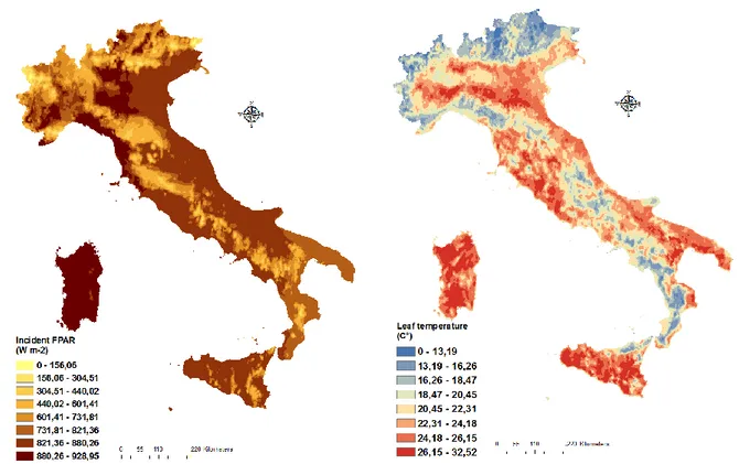
Figure 3-4 Example of the geographic distribution of FPAR and Leaf temperature in Italy obtained for July 29nd, 2006.

Le af T e mp e ra tu re Hours of day

34

4.3 Foliar biomass density

At stand scale the VOC emissions not only depends on the species compositions and the environmental condition, but also on the amount of foliar biomass density present for unit land area. Previous studies considered this parameter as a constant, independently on the phenological estate of the vegetation during the vegetative season. Nevertheless, more information on the seasonal VOC emission dynamics at the national scale can be obtained introducing the LAI as variable: in our work we used the Leaf Area Index (LAI) data for the year 2006, obtained from high resolved satellite observation (MODIS, MODerate-resolution Imaging Spectroradiometer) provided by the partners of the project. The frequency of the satellite observations was 8-day. The foliar biomass density was calculated combining the LAI maps with species-specific value of SLA. To estimate the foliar biomass density we used data collected during recent years along with data previously reported in the literature. For each species the SLA value was considered constant during the year.

Through this procedure we obtained maps of foliar biomass density ( for each class of Table 1-4. The SLA values used for each plant species are reported in Table 3-4 and 4-4. Therefore, the DB was calculated

daily for the year 2006; Figure 4-4 shows an example of DB for the species Q. ilex (Julian day 217, August

07th, 2006). The LAI value with 8-days frequency was integrated in the daily calculation of the emission.

Figure 4-4 Geographic distribution of foliar biomass density in Italy for the Q. ilex species (Values obtained for August 07th, 2006).

Foliar biomass density [g m-2] 1 0 - 240 2 240 - 480 3 480 - 720 4 720 - 960 5 960 - 1200