New non-additive integrals in Multiple Criteria Decision Analysis

(1)

DEPARTMENT OF ECONOMICS AND BUSINESS UNIVERSITY OF CATANIA

NEW NON-ADDITIVE INTEGRALS IN

MULTIPLE CRITERIA DECISION

ANALYSIS

Fabio Rindone

PhD THESIS

Supervisor Prof. Salvatore Greco

INTERNATIONAL PhD in APPLIED MATHEMATICS XXV CYCLE

(2)

New non-additive integrals in

Multiple Criteria Decision Analysis

Fabio Rindone

Department of Economics and Business

University of Catania, Italy

(3)

Preface

Decision has inspired reflection of many thinkers since the ancient times. Often decision is strongly related to the comparison of different points of view, some in favor and some against a certain decision. This means that decision is intrinsically related to a plurality of points of view, which tech-nically are defined criteria. Contrary to this very natural observation, for many years the only way to state a decision problem was considered to be the definition of a single criterion, which amalgamates the multidimensional aspects of the decision situation into a single scale of measure. For exam-ple, even today this approach can be found in any textbooks of Operations Research. This is a very reductive, and in some sense also unnatural, way to look at a decision problem. Thus, for at least thirty years, a new way to look at decision problems has more and more gained the attention of researchers and practitioners. This approach explicitly takes into account the pros and the cons of a plurality of points of view, in other words the domain of Multiple Criteria Decision Analysis (MCDA). Therefore, MCDA intuition is closely related to the way humans have always been making de-cisions. Consequently, despite the diversity of MCDA approaches, methods and techniques, the basic ingredients of MCDA are very simple: a finite or

(4)

infinite set of actions (alternatives, solutions, courses of action, ...), at least two criteria, and, obviously, at least one decision-maker (DM). Given these basic elements, MCDA is an activity which helps making decisions mainly in terms of choosing, ranking or sorting the actions.

MCDA is not just a collection of theories, methodologies, and techniques, but a specific perspective to deal with decision problems. Losing this perspective, even the most rigorous theoretical developments and applications of the most refined methodologies are at risk of being meaningless, because they miss an adequate consideration of the aims and of the role of MCDA. A fundamen-tal problem of MCDA is the representation of preferences. Classically, for example in economics, it is supposed that preference can be represented by a utility function assigning a numerical value to each action such that the more preferable an action, the larger its numerical value. Moreover, it is very often assumed that the comprehensive evaluation of an action can be seen as the sum of its numerical values for the considered criteria. Let us call this the classical model. It is very simple but not too realistic. Indeed, there is a lot of research studying under which conditions the classical model holds. These conditions are very often quite strict and it is not reasonable to assume that they are satisfied in all real world situations. In the last years many non-classical approaches have been proposed in MCDA. This thesis focuses on MCDA methods based on fuzzy integrals. These methods are known in MCDA for the last two decades. In very simple words this methodology permits a flexible modeling of the importance of criteria. Indeed, fuzzy in-tegrals are based on a capacity which assigns an importance to each subset of criteria and not only to each single criterion. Thus, the importance of a

(5)

given set of criteria is not necessarily equal to the sum of the importance of the criteria from the considered subset. Consequently, if the importance of the whole subset of criteria is smaller than the sum of the importances of its individual criteria, then we observe an average redundancy between criteria, which in some way represents overlapping points of view. On the other hand, if the importance of the whole subset of criteria is larger than the sum of the importances of its members, then we observe an average synergy between criteria, the evaluations of which reinforce one another. On the basis of the importance of criteria measured by means of a capacity, the criteria are ag-gregated by means of specific fuzzy integrals, the most important of which are the Choquet integral (for cardinal evaluations) and the Sugeno integral (for ordinal evaluations).

The proposal and the axiomatization of new fuzzy integrals has a central role in modern MCDA. In this thesis we propose some generalizations of well known fuzzy integrals (Choquet, Shilkret and Sugeno). This thesis is thought to make each chapter independent of the others, so they can be read in any order or selected to suit different interests. No general conclusion are given since any chapter contains proper conclusions.

Chapter 1 is a brief survey of the methodology based on fuzzy integrals in MCDA. In chapter 2 we propose and characterize bipolar fuzzy integrals, which are generalization of the most famous fuzzy integrals to the case of bipolar scale, i.e. those symmetric scale where it is possible for each value to find the opposite. Cardinal bipolar scales are intervals [−a, a], ] − ∞, +∞[, while an example of an ordinal bipolar scale is: very bad, bad, neutral, good, very good. In chapter 3 we deal with the generalization of the concept of

(6)

universal integral (recently proposed to generalize several fuzzy integrals) to the case of bipolar scales. We also provide the characterization of the bipo-lar universal integral with respect to a level dependent bi-capacity. Finally, in chapter 4 we consider the problem to adapt classical definitions of fuzzy integrals to the case of imprecise interval evaluations. More precisely, stan-dard fuzzy integrals used in MCDA request that the starting evaluations of a choice on various criteria must be expressed in terms of exact-evaluations. In this last chapter we present the robust Choquet, Shilkret and Sugeno integrals, computed with respect to an interval capacity. These are quite natural generalizations of the Choquet, Shilkret and Sugeno integrals, useful to aggregate interval-evaluations of choice alternatives into a single over-all evaluation. We show that, when the interval-evaluations collapse into exact-evaluations, our definitions of robust integrals collapse into the previ-ous definitions. We also provide an axiomatic characterization of the robust Choquet integral. The approach of robust integral promises interesting de-velopments for future researches, this further improvement is based to the generalization of the concept of interval to h−interval. We shall close the thesis by briefly discussing this last approach.

(7)

Chapter 1 Fuzzy measures and integrals in

MCDA

Grabisch and Labreuche have exhaustively discussed the use of fuzzy measures and integrals in MCDA in literature [16, 17], to which we refer for this chapter.

The aim of MCDA is to model the preferences of a Decision Maker (DM) over a set of possible alternatives X = {x, y, z, . . .} described by several points of view, called criteria N = {1, 2, . . . , n}. Thus, an alternative x is characterized by an evaluation xi ∈ Xi, i= 1, . . . , n (not necessarily numerical) w.r.t. each

point of view and can be identified with a score vector x = (x1, . . . , x_n). We

denote by ⪰ the preference relation of the DM over alternatives, then x ⪰ y means that the DM prefers the alternative x to y . In order to come up with the knowledge of ⪰ on X × X, some informations must be elicited from the DM. This elicitation process should request a relatively small amount of questions asked to the DM. The DM provides informations by means of

(11)

examples of comparisons between alternatives, as well as more qualitative judgments. A numerical representation [33] of the preference ⪰ is obtained whenever there exists a function u∶ X → R such that

∀x, y ∈ X, x ⪰ y iff u(x) ≥ u(y). (1.1)

We focus on a special model of (1.1) called decomposable [29] given by:

u(x) = F(u1(x1), . . . , un(xn)), (1.2)

where the ui are the utility functions and F ∶ Rn→ R is an aggregation func-tion. Krantz et al. [33] (see also [23]) gave the axioms that characterize the representation of ⪰ by (1.2). The weighted sums F(u1, . . . , u_n) = ∑n1αiui are

the most classical functions used to aggregate the criteria. These family of aggregation operators are characterized by an independence axiom [29, 49]. This property implies some limitations in the way the weighted sum can model typical decision behaviors. To make this more precise, we shall provide an example. The construction of the utility functions and the determination of the parameters of the aggregation function are often carried out in two separate steps.

The determination of the utility function is also concerned with commen-surateness between criteria, i.e. the possibility to compare any element of one point of view with any element of any other point of view. This is inter-criteria comparability:

(12)

at least as good as xj by the DM.

This assumption is very strong. By the way of an example, assuming as criteria to buy a car consumption and maximal speed, the DM should be able to say if she prefers a consumption of 5 liters/100km to a maximum speed of 200 km/h. This does not generally make sense to the DM, so that he or she is not generally able to make this comparison directly.

1.1 Notion of Interaction – A Motivating

Ex-ample

In [16] the authors provide the following example to explain the importance of interaction of criteria and to show some flaws of the weighted sum. The director of a university decides on students who are applying for graduate studies in management where some prerequisites from school are required. Students are indeed evaluated according to mathematics, statistics and lan-guage skills. All the marks with respect to the scores are given on the same scale from 0 to 20. These three criteria serve as a basis for a preselection of the candidates. The applicants have generally speaking a strong scientific background so that mathematics and statistics have a big importance to the director. However, he does not wish to favor too much students that have a scientific profile with some flaws in languages. Besides, mathematics and statistics are in some sense redundant, since, usually, students good at math-ematics are also good at statistics. As a consequence, for students good in mathematics, the director prefers a student good at languages to one good

(13)

at statistics. Consider the following four students

Mathematics Statistics Language

student A 16 13 7

student B 16 11 9

student C 6 13 7

student D 6 11 9

Student A is highly penalized by his performance in languages. Henceforth, the director would prefer the student B which has the same mark in mathe-matics but is a little bit better in languages even if he is a little bit worse in statistics. Consider now students C and D. Both of them have a weakness in mathematics. In this case, since the applicants are supposed to have strong scientific skills, the student C which is good in statistics is now preferred to the student D, good in languages. The director preferences, B ⪰ A and C ⪰ D, lead to the following requirement

F(16, 13, 7) < F(16, 11, 9) and F(6, 13, 7) > F(6, 11, 9).

No weighted sum can model such preferences, since the preference of B over A implies that languages is more important than statistics whereas the pref-erence of C over D tells exactly the contrary.

1.2 Capacities and Choquet Integral

The above example suggests that to explain the director preferences we should assign weights not only to the single criteria, but also to the coalitions

(14)

(i.e. groups, subsets) of criteria. This can be achieved by introducing partic-ular functions onP(N), called fuzzy measures [47] or capacities [43]. A fuzzy measure or capacity is a set function µ∶ 2N → R such that µ(∅) = 0, µ(N) = 1

and satisfying the monotonicity condition: if A ⊆ B, then µ(A) ≤ µ(B), for all A, B∈ P(N). The capacity is said to be additive if µ(A∪B) = µ(A)+µ(B), whenever A∩ B = ∅. The Choquet integral [7] of x = (x1, . . . , xn) ∈ Rn w.r.t.

a capacity µ has the following expression :

Ch(x, µ) = ∫

0

−∞[µ{i ∣ xi≥ t} − 1]dt + ∫ ∞

0 µ{i ∣ xi≥ t}. (1.3)

Note that when the capacity is additive, the Choquet integral reduces to a weighted sum. The preference of the DM are modeled via the Choquet integral if

∀x, y ∈ X, x ⪰ y iff Ch(x, µ) ≥ Ch(y, µ). (1.4) Obviously in the (1.4) and according with the (1.2) we have supposed that the component xi of the vector x are expressed n terms of utility. It is easy

to see that the use of the (1.4) applied to the above example of student evalu-ation allows for a simple explanevalu-ation. Indeed, the preferences of the director correspond to 2µ(Mat,Sta)> µ(Mat)+1 and 2µ(Stat) > µ(Stat,Lang). There is no contradiction between previous two inequalities, hence the Choquet integral can model the preferences of the DM. For other properties and char-acterizations of the Choquet integral, we refer the reader to survey papers [35].

(15)

1.3 Conclusions

In the last thirty years several non-additive fuzzy integrals have been developed in MCDA. We recall the Choquet and Shilkret integral (for the cardinal case) and the Sugeno integral (for the ordinal case) among others. In this chapter we have described the Choquet integral in order to show its potentiality in the context of MCDA. In the next chapters we shall present other fuzzy integrals together with their relevant, old and new, generaliza-tions.

(16)

Chapter 2 Bipolar Fuzzy Integrals

2.1 Introduction

The basic reference for this chapter is [25]. In decision analysis and espe-cially in multiple criteria decision analysis, several non additive integrals have been introduced in the last sixty years [8, 10, 16]. Among them, we remember the Choquet integral [7], the Shilkret integral [45] and the Sugeno integral [47]. Recently the bipolar Choquet integral [14, 15, 22] has been proposed for the case in which the underlying scale is bipolar. A further generalization is that of level dependent integrals, which has lead to the definition of the level dependent Choquet integral [21], the level dependent Shilkret integral [4], the level dependent Sugeno integral [37] and the bipolar level dependent Choquet integral [21]. Very recently, on the basis of a minimal set of axioms, one concept of universal integral giving a common framework to many of the above integrals have been proposed [32]. In this chapter we aim to provide a general framework for the case of bipolar fuzzy integrals, i.e. those integrals

(17)

whose underlying scale is bipolar. For this purpose we propose the definition of bipolar Shilkret integral and bipolar Sugeno integral. Then, in order to provide a mathematical characterization of the three mentioned bipolar inte-grals, we give necessary and sufficient conditions for an aggregation function to be the bipolar Choquet integral or the bipolar Shilkret integral or the bipolar Sugeno integral. As we said, the bipolar fuzzy integrals admit a fur-ther generalization if the fuzzy measure (capacity) with respect to which the integrals are calculated can change from a level to another [21, 20]. For the sake of clarity, we shall remind the characterization of the bipolar Shilkret and Sugeno integral with respect to a level dependent capacity in a forth-coming paper (we wish to remember as such results have just been presented in [20]). The chapter is organized as follows. In section 2.2 we give the preliminaries and list some properties of an aggregation function useful to the characterization of the bipolar fuzzy integrals we shall propose in this chapter. In section 2.3 we review the definitions and characterizations of the classical Choquet integral, Shilkret integral, Sugeno integral and some of their symmetric extensions on a bipolar scale. In section 2.4 we give our main results: first we propose the bipolar version of the Shilkret integral and of the Sugeno integral; next we characterize the bipolar Choquet, Shilkret and Sugeno integrals. All the proofs are presented in section 2.5. Section 2.6 contains conclusions.

(18)

2.2 Preliminaries

Let us consider a set of criteria N = {1, . . . , n} and let us suppose that the range of evaluation of given criteria is a real numbers interval I. We denote α= inf I and β = sup I. An alternative can be identified with a score vector x = (x1, . . . , xn) ∈ In, being xi the evaluation of such an alternative x

with respect to the ith _{criterion. An alternative x dominates another y if on}

each criterion the evaluation of x is not smaller than the evaluation of y , i.e. for all i∈ N, xi ≥ yi and in this case we simply write x ≥ y. The indicator

function of any A⊆ N is the function which attains 1 on A and 0 on N ∖ A and can be identified with the vector 1A whose ith component is equal to 1

if i∈ A and 0 otherwise.

In general, an aggregation function is a function G∶ In

→I such that 1. G(α, . . . , α) = α if α ∈ I and limx→α+G(x, . . . , x) = α if α ∉ I;

2. G(β, . . . , β) = β if β ∈ I and limx→β−G(x, . . . , x) = β if β ∉ I;

3. for all x , y ∈ In _{such that x} ≥ y, G(x) ≥ G(y).

In this chapter we often denote the maximum and the minimum of a set X respectively with ⋁X and ⋀X. For any two alternatives x, y ∈ In_{, the}

following definitions hold

• x ∧ y is the vector whose ith component is (x ∧ y)i = ⋀{xi, yi} for all

i = 1, . . . , n (in case y = (h, . . . , h) is a constant, then we can write x ∧ h);

(19)

i = 1, . . . , n (in case y = (h, . . . , h) is a constant, then we can write x ∨ h);

• x and y are comonotone (or comonotonic) if (xi− xj)(yi− yj) ≥ 0 for

all i, j ∈ N;

• x and y are bipolar comonotone if(∣xi∣−∣xj∣)(∣yi∣−∣yj∣) ≥ 0 and xiyi ≥ 0,

for all i, j∈ N.

The following properties of an aggregation function G∶ In

→I are useful to characterize several integrals:

• idempotency: for all a∈ In such that a= (a, . . . , a), G(a) = a;

• homogeneity: for all x ∈ In and c> 0 such that c ⋅ x ∈ In, G(c ⋅ x) = c⋅ G(x);

• stability w.r.t. the minimum: for all x ∈ In and γ ∈ I, G(x ∧ γ) = ⋀{G(x), γ};

• additivity: for all x , y ∈ Insuch that x+y ∈ In, G(x+y) = G(x)+G(y); • maxitivity: for all x , y ∈ In, with α≥ 0, G(x ∨ y) = ⋁{G(x),G(y)}; • minitivity: for all x , y ∈ In, with β≤ 0, G(x ∧ y) = ⋀{G(x),G(y)}; • comonotonic additivity: for all comonotone x , y ∈ In, G(x + y) =

G(x) + G(y);

• comonotonic maxitivity: for all comonotone x , y ∈ In, G(x ∨ y) = ⋁{G(x), G(y)};

(20)

• comonotonic minitivity: for all comonotone x , y ∈ In, G(x ∧ y) = ⋀{G(x), G(y)};

2.3 Fuzzy integrals

In this section we briefly review the three most famous fuzzy integrals, i.e. the Choquet, Shilkret and Sugeno integrals and some of their symmetric extensions. For each of them we shall discuss the restrictions to be imposed on the scale I.

2.3.1 The Choquet integral

Definition 1. A capacity (or fuzzy measure) is function µ ∶ 2N

→ [0, 1] satisfying the following properties:

1. µ(∅) = 0, µ(N) = 1,

2. for all A⊆ B ⊆ N, µ(A) ≤ µ(B).

Definition 2. The Choquet integral [7] of a vector x = (x1, . . . , x_n) ∈ In ⊆

[0, +∞ [n

with respect to the capacity µ is given by

Ch(x, µ) = ∫

∞

0

µ({i ∈ N ∶ xi≥ t})dt. (2.1)

Schmeidler [43] extended the above definition to negative values too, more-over he characterized the Choquet integral in terms of comonotonic additivity and idempotency.

(21)

Definition 3. [43] The Choquet integral of a vector x= (x1, . . . , xn) ∈ Inwith

respect to the capacity µ is given by

Ch(x, µ) = ∫

0

−∞(µ ({i ∈ N ∶ xi≥ t}) − 1)dt + ∫ ∞

0 µ({i ∈ N ∶ xi≥ t})dt. (2.2)

Alternatively (2.2) can be written as [21]

Ch(x, µ) = ∫

max_ixi

min_i_x_i µ({i ∈ N ∶ xi≥ t})dt + mini xi. (2.3)

Another formulation of (2.2) can be obtained, by using the summation, as

Ch(x, µ) =

n

∑

i=2(x

σ(i)− xσ(i−1)) ⋅ µ ({j ∈ N ∶ xj ≥ xσ(i)}) + xσ(1), (2.4)

being σ ∶ N → N any permutation of indexes such that xσ(1)≤ . . . ≤ xσ(n).

Theorem 1. [43] An aggregation function G ∶ In

→ I is idempotent and comonotone additive if and only if there exists a capacity µ such that, for all x∈ In_,

G(x) = Ch(x, µ).

The ˇSipoˇs integral [46] (or symmetric Choquet integral) of x ∈ In_{with respect}

to the capacity µ is defined by

ˇ

Ch(x, µ) = Ch(x ∨ 0, µ) − Ch(−(x ∧ 0), µ). (2.5) More in general, a functional L∶In

(22)

func-tional [39] if there exist two fuzzy measures µ+ _{and µ}−_{such that for all x} ∈ In

L(x) = Ch(x ∨ 0, µ+) − Ch(−(x ∧ 0), µ−).

This functional is used in the cumulative prospect theory [48]. Clearly when µ+ = µ−_{, the rank and sign-dependent functional L is exactly the}

symmet-ric Choquet integral. For further details on the rank and sign-dependent functional and its use in cumulative prospect theory, we refer the reader to [48, 39]. We wish also to remember that Choquet integral is generalized and characterized in [2, 3].

2.3.2 The Shilkret integral

Definition 4. The Shilkret integral [45] of a vector x = (x1, . . . , x_n) ∈ In ⊆

[0, +∞ [n

with respect to the capacity µ is given by

Sh(x, µ) = ⋁

i∈N{xi⋅ µ({j ∈ N ∶ xj≥ xi})}.

(2.6)

A generalization of the Shilkret integral is introduced and characterized in [2, 3]. From the cited papers we can get a characterization of the Shilkret integral in terms of idempotency, comonotonic maxitivity and homogeneity. For the sake of completeness we report the proof of such a characterization (Theorem 2) in section 2.5.

Theorem 2. Suppose that α = inf I ≥ 0, then an aggregation function G ∶ In

(23)

there exists a capacity µ on N such that, for all x∈ In_,

G(x) = Sh(x, µ).

Although in [45] the Shilkret integral was formulated for nonnegative func-tions, however (2.6) works also for a generic x ∈ In⊆ Rn_{. But, in our opinion,}

if we allow for negative values too, the essence of the Shilkret integral is lost. Let us stress this point with some examples. Suppose that an alternative is strongly negatively evaluated on each criterion except on the last, where it has a low nonnegative evaluation, e.g. x = (−100, −100, −100, 1). By ap-plying (2.6), Sh(x, µ) = µ ({4}), for every capacity µ. Thus, the negative evaluations and the weights that the capacity assigns to the relative criteria with respect to which these negative evaluations are given, are ininfluent on the evaluation of x . In general, if for a given alternative x we have simulta-neously negative and positive evaluations on the various criteria, the negative ones are ininfluent and the Shilkret integral of x coincides with the Shilkret integral of x ∨ 0. In the case of x ∈ ] − ∞, 0[n it is straightforward noting that Sh(x, µ) = (maxi∈Nxi) ⋅ µ ({j ∈ N ∣ xj≥ maxi∈Nxi}). Again, we note

how for all capacities only the maximum evaluation of x matters. For vec-tors with non-positive evaluation on each criterion, the logic of the Shilkret integral can be recovered if in the (2.6) we substitute the maximum with the minimum and ≥ with ≤.

(24)

In⊆ ] − ∞, 0]n _{with respect to the capacity µ is given by} Sh−(x, µ) = ⋀ i∈N{xi⋅ µ({j ∈ N ∶ xj≤ xi})} = −⋁ i∈N{−x i⋅ µ({j ∈ N ∶ −xj ≥ −xi})} = −Sh(−x, µ). (2.7)

Obviously, from theorem 2, the characterization of the negative Shilkret in-tegral is in terms of idempotency, comonotonic minitivity and homogeneity.

Corollary 1. Suppose that β = sup I ≤ 0, then an aggregation function G ∶ In

→I is idempotent, comonotone minitive and homogeneous if and only if there exists a capacity µ on N such that, for all x∈ In_,

G(x) = Sh−(x, µ).

So far, we have a Shilkret integral for alternatives with all non-negative evaluations and one for alternatives with all non-positive evaluations. To obtain a suitable definition of the Shilkret integral for the mixed case we propose two different approaches. In the first approach we define a symmetric Shilkret integral by applying a logic `a la ˇSipoˇs [46], i.e. for all x ∈ I

ˇ

Sh(x, µ) = Sh(x ∨ 0, µ) + Sh−(x ∧ 0, µ).

(2.8)

Note that the (2.8) is called symmetric since ˇSh(x, µ) = −ˇSh (−x, µ). A second, more general, approach will be to define a bipolar Shilkret integral (see next section). This would be used directly for the bipolar scale, while

(25)

restricted on R+ _{and on R}− _{it would coincide respectively with the Shilkret}

integral and the negative Shilkret integral.

2.3.3 The Sugeno integral

Definition 6. A measure on N with a scale I is any function ν ∶ 2N

→I such that:

1. ν(∅) = α = inf I, ν(N) = β = sup I, 2. for all A⊆ B ⊆ N, ν(A) ≤ ν(B).

Definition 7. The Sugeno integral [47] of a vector x= (x1, . . . , xn) ∈ In with

respect to the measure ν on N with scale I is given by Su(x, ν) = ⋁

i∈N⋀{xi

, ν({j ∈ N ∣ xj ≥ xi})}. (2.9)

Alternatively the Sugeno integral can be written as

Su(x, ν) = ⋁

A⊆N⋀{ν(A), ⋀i∈A

xi}. (2.10)

Next theorem gives necessary and sufficient conditions for an aggregation function to be the Sugeno integral.

Theorem 3. [36] An aggregation function G∶In

→I is idempotent, comono-tone maxitive and stable with respect to the minimum if and only if there

(26)

exists a measure ν on N with a scale I such that, for all x ∈ In_,

G(x) = Su(x, ν).

Let us observe that the definition of the Sugeno integral only imposes that the xi and the ν(A) are measured on the same (possible only ordinal) scale

I. For further generalization and characterization of the Sugeno integral see [2, 3].

Let us consider the symmetric scale [−1, 1]. The symmetric maximum of two elements a, b ∈ [−1, 1] - introduced and discussed in [11, 12] - is defined by the following binary operation:

a 6 b= ⎧⎪⎪⎪⎪ ⎪⎪⎪⎪ ⎨⎪⎪⎪ ⎪⎪⎪⎪⎪ ⎩

− (∣a∣ ∨ ∣b∣) if b≠ −a and either ∣a∣ ∨ ∣b∣ = −a or = −b

0 if b= −a

∣a∣ ∨ ∣b∣ else.

Alternatively the symmetric maximum can be written as

a 6 b= sign(a + b)(∣a∣ ∨ ∣b∣).

The symmetric minimum of two elements [11, 12] is defined as:

a 7 b= ⎧ ⎪ ⎪ ⎪ ⎪ ⎨ ⎪ ⎪ ⎪ ⎪ ⎩

− (∣a∣ ∧ ∣b∣) if sign(b)≠ sign(a) ∣a∣ ∧ ∣b∣ else.

(27)

a 7 b= sign(a ⋅ b)(∣a∣ ∧ ∣b∣). Suppose that µ ∶ 2N

→ [0, 1] is a capacity and x ∈ [−1, 1]n is a vector evaluated on each criterion on the symmetric scale [−1, 1]. The symmetric Sugeno integral [11] of x is defined as

ˇ

Su(x, µ) = (Su(x ∨ 0, µ)) 6 (−Su((−x) ∨ 0, µ)). (2.11) In (2.11), as before in (2.8), symmetric means that ˇSu(x, µ) = −ˇSu (−x, µ). Clearly if xi ≥ 0 for all i ∈ N, ˇSu (x, µ) = Su(x, µ), while if xi≤ 0 for all i ∈ N,

ˇ

Su(x, µ) = ⋀

i∈N⋁{xi

,−ν({j ∈ N ∣ xj ≤ xi})}. (2.12)

(2.12) can be considered as a definition of a negative Sugeno integral, for the case in which x is negatively evaluated on each criterion.

In [41] the notion of symmetric Sugeno integral has been extended.

Definition 8. A functional L ∶ [−1, 1]n → [−1, 1] is a fuzzy rank and sign-dependent functional if there exist two fuzzy measures µ+ _{and µ}− _{such that}

for all x∈ [−1, 1]n

L(x) = (Su(x ∨ 0, µ+)) 6 (−Su((−x) ∨ 0, µ−)).

(2.13)

Clearly when µ+ = µ−_{, the fuzzy rank and sign-dependent functional L is}

exactly the symmetric Sugeno integral. For further details on the fuzzy rank and sign-dependent functional and on the symmetric Sugeno integral we refer

(28)

the reader to [11, 41].

In the next section we shall propose a more general approach, defining a bipo-lar Sugeno integral, which restricted on R+ _{and on R}− _{coincides respectively}

with the (7) and the (2.12).

2.4 Bipolar fuzzy integrals on the scale [-1,1]

The present work is devoted to the study of bipolar fuzzy integrals, i.e. those integrals useful when the scale underlying the alternatives evaluation is bipolar. For the sake of simplicity, trough this section we shall adopt the bipolar scale [−1, 1] to present our results. However, without loss of the gen-erality, they can be extended to every other symmetric interval of R, i.e. any of [−α, α], ] − α, α[, ] − ∞, +∞[, where α ∈ R+_.

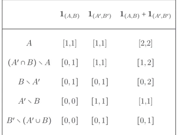
Let us consider the set Q = {(A, B) ∈ 2N_{× 2}N _{∶ A ∩ B} = ∅} of all disjoint

pairs of subsets of N . With respect to the binary relation (A, B) ≾ (C, D) iff A⊆ C and B ⊇ D, Q is a lattice, i.e. a partial ordered set in which any two elements have a unique supremum, (A, B) ∨ (C, D) = (A ∪ C, B ∩ D), and a unique infimum, (A, B)∧(C, D) = (A ∩ C, B ∪ D). For all (A, B), (C, D) ∈ Q if A⊆ C and B ⊆ D, we simply write (A, B) ⊆ (C, D). For all (A, B) ∈ Q the indicator function 1_(A,B) ∶ N →{−1, 0, 1} is the function which attains 1 on A, -1 on B and 0 on (A ∪ B)c. Such a function can be identified with the vector 1_(A,B) whose ith_{component is equal to 1 if i}∈ A, is equal to −1 if i ∈ B

and is equal to 0 otherwise.

In [38] it has been shown that the symmetric maximum 6∶[−1, 1]×[−1, 1] → [−1, 1] coincides with two recent symmetric extensions of the Choquet

(29)

inte-gral, the balancing Choquet integral and the fusion Choquet inteinte-gral, when they are computed with respect to the strongest capacity (i.e. the capac-ity ν ∶ 2N

→[0, 1] which attains zero on the empty set and one elsewhere). However, the symmetric maximum of a set X cannot be defined, being > non associative; e.g, suppose that X = {3, −3, 2}, then (3 6 −3) 6 2 = 2 or 3 6(−3 6 2) = 0, depending on the order. Several possible extensions of the symmetric maximum for dimension n, n> 2 have been proposed (see [12, 18] and also the related discussion in [38]). One of these extensions is based on the splitting rule applied to the maximum and to the minimum as described in the following. Given X = {x1, . . . , x_m} ⊆ R, the bipolar maximum of X,

shortly ⋁b_{X, is defined as:}

⋁b X= m ⋁ i b_x i = ( m ⋁ i xi) > ( m ⋀ i xi). (2.14)

The following definitions are closely related to the above discussion.

Definition 9. Given X = {x1, . . . , x_m} ⊆ R, the positive bipolar maximum

of X, shortly ⋁b+_{X, is the element with the greatest absolute value, with}

the convention that, in the case of two different opposite elements with this property, we choose the non-negative.

Definition 10. Given X = {x1, . . . , xm} ⊆ R, the negative bipolar maximum

of X, shortly ⋁b−X, is the element with the greatest absolute value, with the convention that, in the case of two different opposite elements with this property, we choose the non-positive.

Following these definitions, if X = {9, −9, 7, −3} thus, ⋁b_X = 0, ⋁b+_X= 9 and

(30)

the relation: ⋁bX= ⋁b{⋁b+X,⋁b−X}. Given the vectors x1

, . . . , xk∈ [−1.1]n_{with K} = {1, . . . , k}, ⋁b

j∈Kxj is the vector

whose ith _{component is}⋁b{x1

i, . . . , xki} for all i = 1, . . . , n.

The following properties of an aggregation function G∶[−1, 1]n→[−1, 1] are useful to characterize several bipolar integrals.

• bipolar comonotonic additivity: for all bipolar comonotone x , y ∈ [−1, 1]n

,

G(x + y) = G(x) + G(y);

• bipolar stability of the sign: for all r, s∈]0, 1] and for all (A, B) ∈ Q, G(r1A,B)G(s1A,B) > 0 or G(r1A,B) = G(s1A,B) = 0,

i.e., in simple words, G(r1_(A,B)) and G(s1_(A,B)) have the same sign; • bipolar stability with respect to the minimum: for all r, s ∈]0, 1] such

that r > s, and for all (A, B) ∈ Q, ∣G(r1(A,B))∣ ≥ ∣G(s1(A,B))∣ and,

moreover,

if ∣G(r1_(A,B))∣ > ∣G(s1_(A,B))∣ then ∣G(s1_(A,B))∣ = s.

2.4.1 A specific property: bipolar comonotone

maxi-tivity

With a slight abuse of notation we extend the relation of set inclusion to Q, by defining (A, B) ⊆ (C, D) if and only if A ⊆ C and B ⊆ D, for all

(31)

(A, B), (C, D) ∈ Q. Let us suppose to have k different levels l1, . . . , lk∈ R with

0< l1< l2 < . . . < l_k≤ 1 and a sequence {(A_i, B_i)}_i_=1,...,k such that(A_i, B_i) ∈ Q

for all i = 1, . . . , k and (Ai+1, Bi+1) ⊆ (Ai, Bi) for all i = 1, . . . , k − 1. The

vectors li⋅ 1(Ai,Bi), i = 1, . . . , k are bipolar comonotonic and, moreover, by

ordering them with respect to the level li, then in the vector li⋅ 1(Ai,Bi), for

each component the elements under the level li are the opposite of that under

the level −li. See for example the four vectors

x = (7, −7, 0, 0) y = (5, −5, 5, 0) w= (3, −3, 3, −3) z = (2, −2, 2, −2).

An aggregation function G is said to be bipolar comonotone maxitive if it is maxitive on such a type of bipolar comonotonic bi-constants, i.e. if fixed K = {1, . . . , k} it holds: G(⋁ i∈K b li⋅ 1(Ai,Bi)) = ⋁ i∈K b G(li⋅ 1(Ai,Bi)). (2.15)

G is said to be right bipolar comonotone maxitive if

G(⋁ i∈K b+ li⋅ 1_(Ai,Bi)) = ⋁ i∈K b+ G(li⋅ 1_(Ai,Bi)). (2.16)

G is said to be left bipolar comonotone maxitive if

G(⋁ i∈K b− li⋅ 1_(Ai,Bi)) = ⋁ i∈K b− G(li⋅ 1_(Ai,Bi)). (2.17)

(32)

Clearly, due to bipolar comonotonicity, in equations (2.15)-(2.17): ⋁ i∈K b li⋅ 1(Ai,Bi)= ⋁ i∈K b+ li⋅ 1(Ai,Bi)= ⋁ i∈K b− li⋅ 1(Ai,Bi).

2.4.2 The bipolar Choquet integral

Definition 11. A function µb ∶Q → [−1, 1] is a bi-capacity [14, 15, 22] on

N if

• µb(∅, ∅) = 0, µb(N, ∅) = 1 and µb(∅, N) = −1;

• µb(A, B) ≤ µb(C, D) ∀ (A, B), (C, D) ∈ Q such that (A, B) ≾ (C, D).

Definition 12. The bipolar Choquet integral of x = (x1, . . . , x_n) ∈ [−1, 1] n

with respect to the bi-capacity µb is given by [14, 15, 22, 21]:

Chb(x, µb) = ∫ ∞

0 µb({i ∈ N ∶ xi> t}, {i ∈ N ∶ xi< −t})dt. (2.18)

The bipolar Choquet integral of x = (x1, . . . , xn) ∈ [−1, 1] n

with respect to the bi-capacity µb can be rewritten as

Chb(x, µb) = n

∑

i=1(∣x

σ(i)∣ − ∣xσ(i−1)∣)µb({j ∣ xj ≥ ∣xσ(i)∣}, {j ∣ xj≤ −∣xσ(i)∣}),

(2.19) being σ∶ N → N any permutation of index such that 0 = ∣xσ(0)∣ ≤ ∣xσ(1)∣ ≤ . . . ≤

∣xσ(n)∣. Note that to ensure that the pair ({j ∈ N ∶ xj ≥ ∣t∣}, {j ∈ N ∶ xj ≤ −∣t∣})

(33)

maintained trough all the chapter - that in the case of t = 0 the inequality xj ≤ 0 is to be understood as xj < 0. The formulation (2.19) will be useful in

proving some results, like that exposed in the next representation theorem.

Theorem 4. [22] An aggregation function G∶ [−1, 1]n→[−1, 1] is idempotent and bipolar comonotonic additive if and only if there exists a bi-capacity µb

such that, for all x∈ [−1, 1]n,

G(x) = Chb(x, µb).

Remark 1. Although the bipolar Choquet integral is trivially homogeneous, this condition does not appear in the theorem, since an aggregation function which is idempotent and bipolar comonotone additive is also homogeneous. Observe also that we could relax idempotency with the conditions G(1_(N,∅)) = 1 and G(1_(∅,N)) = −1.

2.4.3 The bipolar Shilkret integral

Definition 13. The bipolar Shilkret integral of x = (x1, . . . , xn) ∈ [−1, 1]n

with respect to the bi-capacity µb is given by:

Shb(x, µb) = ⋁ i∈N b

{∣xi∣ ⋅ µb({j ∈ N ∶ xj ≥ ∣xi∣}, {j ∈ N ∶ xj ≤ −∣xi∣})}. (2.20)

Definition 14. The right bipolar Shilkret integral of

x= (x1, . . . , x_n) ∈ [−1, 1] n

(34)

with respect to the bi-capacity µb is given by: Sh+ b(x, µb) = ⋁ i∈N b+ {∣xi∣ ⋅ µb({j ∈ N ∶ xj ≥ ∣xi∣}, {j ∈ N ∶ xj ≤ −∣xi∣})}. (2.21)

Definition 15. The left bipolar Shilkret integral of x= (x1, . . . , xn) ∈ [−1, 1] n

with respect to the bi-capacity µb is given by:

Sh−

b(x, µb) = ⋁ i∈N

b−

{∣xi∣ ⋅ µb({j ∈ N ∶ xj ≥ ∣xi∣}, {j ∈ N ∶ xj ≤ −∣xi∣})}. (2.22)

Clearly the three definitions are linked via the

Shb(x, µb) = ⋁ b

{Sh+

b(x, µb), Sh−b(x, µb)}.

The condition Shb(x, µb) = 0 is equivalent to the Sh+_b(x, µb) = −Sh−_b(x, µb)

and, in this case, either the three integrals are all zero or they give three different results, one zero, one positive and one negative. We can think about them in terms of a neutral, an optimistic and a pessimistic aggregate evaluation of x . The condition Shb(x, µb) ≠ 0 implies that Sh+b(x, µb) =

Sh−

b(x, µb) = Shb(x, µb).

The following theorems characterize the bipolar Shilkret integral.

Theorem 5. An aggregation function G ∶ [−1, 1]n → [−1, 1] is idempotent, bipolar comonotone maxitive and homogeneous if and only if there exists a bi-capacity µb on N such that, for all x∈ [−1, 1]

n

,

(35)

Remark 2. Let us note that theorem 5 implies, as corollary, theorem 2 since bipolar comonotone maxitivity restricted on R+ _{implies comonotone}

maxitivity.

Theorem 6. An aggregation function G ∶ [−1, 1]n → [−1, 1] is idempotent, positive bipolar comonotone maxitive and homogeneous if and only if there exists a bi-capacity µb on N such that, for all x∈ [−1, 1]

n

,

G(x) = Sh+

b(x, µb).

Theorem 7. An aggregation function G ∶ [−1, 1]n → [−1, 1] is idempotent, negative bipolar comonotone maxitive and homogeneous if and only if there exists a bi-capacity µb on N such that, for all x∈ [−1, 1]

n

,

G(x) = Sh−

b(x, µb).

Remark 3. Idempotency could be relaxed with the conditions G(1_(N,∅)) = 1 and G(1_(∅,N)) = −1, in fact from these and from homogeneity idempotency can be elicited.

(36)

2.4.4 The bipolar Sugeno integral

Definition 16. The bipolar Sugeno integral of a vector x = (x1, . . . , x_n) ∈

[−1, 1]n

with respect to the bi-capacity µb on N is given by:

Sub(x, µb) = ⋁ i∈N b

{∣xi∣ 7 µb({j ∈ N ∶ xj ≥ ∣xi∣}, {j ∈ N ∶ xj≤ −∣xi∣})}. (2.23)

Definition 17. The right bipolar Sugeno integral of x= (x1, . . . , x_n) ∈ [−1, 1] n

Su+

b(x, µb) = ⋁ i∈N

b+

{∣xi∣ 7 µb({j ∈ N ∶ xj ≥ ∣xi∣}, {j ∈ N ∶ xj ≤ −∣xi∣})}. (2.24)

Definition 18. The left bipolar Sugeno integral of a vector x= (x1, . . . , xn) ∈

[−1, 1]n

Su−

b(x, µb) = ⋁ i∈N

b−

{∣xi∣ 7 µb({j ∈ N ∶ xj ≥ ∣xi∣}, {j ∈ N ∶ xj ≤ −∣xi∣})}. (2.25)

Clearly the three definitions are linked via the

Sub(x, µb) = ⋁ b

{Su+

b(x, µb), Su−b(x, µb)}.

The condition Sub(x, µb) = 0 is equivalent to the Su+_b(x, µb) = −Su−_b(x, µb)

and, in this case, either the three integrals are all zero or they give three different results, one zero (neutral), one positive (optimistic) and one neg-ative (pessimistic). The condition Sub(x, µb) ≠ 0 implies that Su+_b(x, µb) =

Su−

b(x, µb) = Sub(x, µb).

(37)

Theorem 8. An aggregation function G ∶ [−1, 1]n → [−1, 1] is idempotent, bipolar comonotone maxitive, bipolar stable with respect to the sign and bipo-lar stable with respect to the minimum if and only if there exists a bi-capacity µb on N such that, for all x∈ [−1, 1]

n

,

G(x) = Sub(x, µb).

Theorem 9. An aggregation function G ∶ [−1, 1]n → [−1, 1] is idempotent, positive bipolar comonotone maxitive, bipolar stable with respect to the sign and bipolar stable with respect to the minimum if and only if there exists a bi-capacity µb on N such that, for all x∈ [−1, 1]

n

,

G(x) = Su+

b(x, µb).

Theorem 10. An aggregation function G∶[−1, 1]n→[−1, 1] is idempotent, negative bipolar comonotone maxitive, bipolar stable with respect to the sign and bipolar stable with respect to the minimum if and only if there exists a bi-capacity µb on N such that, for all x∈ [−1, 1]

n

,

G(x) = Su−

(38)

2.5 Proofs of theorems

Proof of Theorem 2.

First we prove the necessary part. Let us suppose there exists a capacity µ on N such that, for all x ∈ In_{, G}(x) = Sh(x, µ). In this case it is trivial

to prove that the Shilkret integral is idempotent, comonotone maxitive and homogeneous by definition and we leave the proof to the reader. Now we prove the sufficient part of the theorem. Let us define

µ(A) = G(1A), for all A ∈ 2N. (2.26)

Because G is an idempotent aggregation function, we get µ(∅) = 0, µ(N) = 1 and µ(A) ≤ µ(B) whenever A ⊆ B. Thus µ is a capacity on N. Every x = (x1, . . . , x_n) ∈ In can be written as

x = ⋁

i∈N

xσ(i)⋅ 1{j∈N ∣ xj≥xσ(i)}

being σ ∶ N → N any permutation of index such that xσ(1) ≤ . . . ≤ xσ(n).

Because vectors xσ(i)⋅ 1{j∈N ∣ xj≥xσ(i)} are comonotonic, we get the thesis by

applying comonotonic maxitivity, homogeneity of G and the definition of µ according to (2.26): G(x) = G (⋁ i∈N xσ(i)⋅ 1{j∈N ∣ xj≥xσ(i)}) = ⋁ i∈N G(xσ(i)⋅ 1{j∈N ∣ xj≥xσ(i)}) = = ⋁ i∈N xσ(i)⋅ G(1{j∈N ∣ xj≥xσ(i)}) = ⋁ i∈N xσ(i)⋅ µ({j ∈ N ∣ xj ≥ xσ(i)}) = Sh(x,µ) ◻

(39)

Proof of Theorem 4.

First we prove the necessary part. Let us suppose that there exists a bi-capacity µb such that, for all x ∈ [−1, 1]

n

, G(x) = Chb(x, µb).

Idempo-tency of the bipolar Choquet integral follows from definition, because if λ ≥ 0, then Chb(λ ⋅ 1(N,∅), µb) = ∫ λ 0 µb(N, ∅)dt = λ, while if λ < 0, then Chb(λ ⋅ 1_(N,∅), µb) = ∫ −λ 0 µb(∅, N)dt = λ. If x, y ∈ [−1, 1] n are bipolar comonotone, then there exists a permutation of indexes σ ∶ N → N such that 0= ∣xσ(0)∣ ≤ ∣xσ(1)∣ ≤ . . . ≤ ∣xσ(n)∣ and 0 = ∣yσ(0)∣ ≤ ∣yσ(1)∣ ≤ . . . ≤ ∣yσ(n)∣, and

then

Chb(x, µb) = n

∑

i₌₁

(∣xσ(i)∣ − ∣xσ(i−1)∣) ⋅ µb({j ∣ xj ≥ ∣xσ(i)∣}, {j ∣ xj ≤ −∣xσ(i)∣}),

and

Chb(y, µb) = n

∑

i=1(∣y

σ(i)∣ − ∣yσ(i−1)∣) ⋅ µb({j ∣ yj≥ ∣yσ(i)∣}, {j ∣ yj ≤ −∣yσ(i)∣}).

Since x and y are absolutely comonotonic an cosigned, for every i= 1, . . . , n µb({j ∈ N ∶ xj ≥ ∣xσ(i)∣}, {j ∈ N ∶ xj ≤ −∣xσ(i)∣}) =

(40)

Moreover, again because x and y are absolutely comonotonic and cosigned, for every i= 1, . . . , n, ∣xσ(i)+ yσ(i)∣ = ∣xσ(i)∣ + ∣yσ(i)∣ and consequently

0= ∣xσ(0)+ yσ(0)∣ ≤ ∣xσ(1)+ yσ(i)∣ ≤ . . . ≤ ∣xσ(n)+ yσ(n)∣ for every i = 1, . . . , n.

(2.28) By (2.27) and (2.28) we get Chb(x, µb) + Chb(y, µb) = Chb(x + y, µb).

Now we prove the sufficient part of the theorem. Let us define

µb(A, B) = G (1(A,B)), for all (A,B) ∈ Q. (2.29)

µb represents a bi-capacity, since by idempotency of G we get that µb(N, ∅) =

G(1_(N,∅)) = 1, µb(∅, N) = G (1(∅,N)) = −1, µb(∅, ∅) = G (1(∅,∅)) = 0.

More-over, if (A, B) ≾ (A′_{, B}′), being for all i ∈ N, the ith _{component of the vector}

1_(A,B) not greater than the ith _{component of the vector 1}

(A′_,B′₎ and being G

an aggregation function (then monotone), thus µb(A, B) ≤ µb(A′, B′).

Ob-serve now that any vector x = (x1, . . . , xn) ∈ [−1, 1]n can be rewritten as

x =

n

∑

i=1(∣x

σ(i)∣ − ∣xσ(i−1)∣) ⋅ 1({j∈N∶xj≥∣xσ(i)∣},{j∈N∶xj≤−∣xσ(i)∣}), (2.30)

being σ ∶ N → N any permutation of indexes such that 0= ∣xσ(0)∣ ≤ ∣xσ(1)∣ ≤

. . .≤ ∣xσ(n)∣. Let us note that for all (A, B), (A′, B′) ∈ Q such that (A, B) ⊆

(A′_{, B}′) and for all a, b ∈ [0, 1], vectors a ⋅ 1

(A,B) and b⋅ 1(A′_,B′₎ are bipolar

comonotone. Consequently, (2.30) shows that any vector x ∈ [−1, 1]n can be decomposed as a sum of bipolar comonotonic vectors. Remembering that an aggregation function which is idempotent and bipolar comonotone additive is also homogeneous, thus to get the thesis it is sufficient to apply, respectively,

(41)

bipolar comonotone additivity, homogeneity of G and definition of bi-capacity µb according to (2.29): G(x) = G ( n ∑ i₌₁

(∣xσ(i)∣ − ∣xσ(i−1)∣) ⋅ 1({j∈N∶xj≥∣xσ(i)∣},{j∈N∶xj≤−∣xσ(i)∣})) =

=∑n

i=1(∣x

σ(i)∣ − ∣xσ(i−1)∣) ⋅ G (1({j∈N∶xj≥∣xσ(i)∣},{j∈N∶xj≤−∣xσ(i)∣})) = Chb(x, µb).

◻

Proof of Theorem 5.

First we prove the necessary part. Let us suppose there exists a bi-capacity µb such that, for all x ∈ [−1, 1]

n

, G(x) = Shb(x, µb). The bipolar Shilkret

in-tegral is, trivially, idempotent and homogeneous and we only need to demon-strate the bipolar comonotonic maxitivity. Let us consider a set of indexes K = {1, . . . , k}, k increasing levels l1, . . . , lk ∈ R with 0 < l1 < l2 < . . . < lk ≤

1 and a sequence {(Ai, Bi)}i∈K such that (Ai, Bi) ∈ Q and (Ai+1, Bi+1) ⊆

(Ai, Bi) for all i ∈ K. The jth component of the vector ⋁bi∈K{li⋅ 1(Ai,Bi)} is

equal to li if j∈ Ai∖ Ai+1, is equal to −li if j ∈ Bi∖ Bi+1 and is equal to zero

if j ∈ N ∖ (A1∪ B1) for all i ∈ K and taking A_k+1 = B_k+1 = ∅. Clearly, such

a vector has a component greater or equal to li for indexes in Ai and has

component smaller or equal to −li for indexes in Bi. Thus, by definition

Shb(⋁ i∈K b {li⋅ 1(Ai,Bi)}, µb) = ⋁ i∈K b {li⋅ µb((Ai, Bi))} = ⋁ i∈K b {Shb(li⋅ 1(Ai,Bi), µb)}. (2.31)

(42)

Now we prove the sufficient part of the theorem. Let us define

µb(A, B) = G (1(A,B)), for all (A,B) ∈ Q. (2.32)

µb represents a bi-capacity (see proof of theorem 4). Notice that each x ∈

[−1, 1]n can be rewritten as x = ⋁ i∈N b ∣xi∣ ⋅ 1({j ∣ xj≥∣xi∣},{j ∣ xj≤−∣xi∣}) (2.33)

and observe that vectors∣xi∣⋅1({j∈N ∣ xj≥∣xi∣},{j∈N ∣ xj≤−∣xi∣}), i= 1 . . . , n are

bipo-lar comonotone. Consequently, for any x ∈ [−1, 1]n by bipolar comonotone maxitivity, homogeneity and definition of bi-capacity µb according to the

(2.32) we get G(x) = G (⋁ i∈N b ∣xi∣ ⋅ 1({j ∣ xj≥∣xi∣},{j ∣ xj≤−∣xi∣})) = ⋁ i∈N b G(∣xi∣ ⋅ 1({j ∣ xj≥∣xi∣},{j ∣ xj≤−∣xi∣})) = = ⋁ i∈N b ∣xi∣ ⋅ G (1({j ∣ xj≥∣xi∣},{j ∣ xj≤−∣xi∣})) = ⋁ i∈N b ∣xi∣ ⋅ µb({j ∣ xj ≥ ∣xi∣}, {j ∣ xj ≤ −∣xi∣}) = Shb(x, µb) ◻

Proof of Theorems 6 and 7. They are analogous to the proof of previous Theorem 5.

(43)

Proof of Theorem 8. First we prove the necessary part. Let us suppose there exists a bi-capacity µb such that, for all x ∈ [−1, 1]

n

, G(x) = Sub(x, µb). The

Sugeno integral is idempotent by definition. Bipolar stability with respect to the sign and with respect to the minimum are trivially verified once we consider that for all r> 0 and for all (A, B) ∈ Q

Sub(r ⋅ 1(A,B), µb) = sign(µb(A, B))⋀{r,∣µb(A, B)∣}.

Let us consider a set of indexes K = {1, . . . , k}, k increasing levels l1, . . . , lk∈

R with 0 < l1 < l2 < . . . < lk ≤ 1 and a sequence {(Ai, Bi)}_i_∈K such that

(Ai, Bi) ∈ Q and (Ai+1, Bi+1) ⊆ (Ai, Bi) for all i ∈ K. Thus, by definition

Sub( ⋁ i∈K b {li⋅ 1_(Ai,Bi)}, µb) = ⋁ i∈K b

{sign [µb((Ai, Bi))] ⋀{li,∣µb((Ai, Bi)) ∣}} =

= ⋁

i∈K b

{Sub(li⋅ 1_(Ai,Bi), µb)}. (2.34)

Now we prove the suﬃcient part of the theorem. Let us deﬁne µb(A, B) =

G(1_(A,B)) for all (A, B) ∈ Q. µb represents a bi-capacity (see proof of

theo-rem 4). Let us note that using bipolar stability with respect to the minimum and idempotency of G we have that for all r > 0 and for all (A, B) ∈ Q,

∣G (r ⋅ 1(A,B))∣ = ⋀{r, ∣G(1(A,B))∣} . (2.35)

The (2.35) is obvious if r = 0 or r = 1. If 0 < r < 1 and∣G (1_(A,B))∣ > ∣G (r ⋅ 1_(A,B))∣, then using stability w.r.t. the minimum, ∣G (r ⋅ 1_(A,B))∣ = r and the (2.35) is true again. If ∣G (1_(A,B))∣ = ∣G (r ⋅ 1_(A,B))∣ observe that by monotonicity and idempotency of G, ∣G (r ⋅ 1_(A,B))∣ ≤ ∣G (r ⋅ 1_(N,∅))∣ = r, which means that also in this last case the (2.35) is true. Finally, notice that each x ∈ [−1, 1]n can be

(44)

rewritten as

x = ⋁

i∈N b_∣x

i∣ ⋅ 1_{({j ∣ x}j≥∣xi∣},{j ∣ xj≤−∣xi∣}) (2.36)

and observe that vectors∣xi∣ ⋅ 1_{({j∈N ∣ x}j≥∣xi∣},{j∈N ∣ xj≤−∣xi∣}), i = 1 . . . , n are bipolar

comonotone.

Consequently, for any x ∈[−1, 1]n by bipolar comonotone maxitivity G(x) = G ( ⋁ i∈N b ∣xi∣ ⋅ 1_{({j ∣ x}j≥∣xi∣},{j ∣ xj≤−∣xi∣})) = ⋁ i∈N b G(∣xi∣ ⋅ 1_{({j ∣ x}j≥∣xi∣},{j ∣ xj≤−∣xi∣})) =

( by bipolar stability with respect to the sign ) = ⋁ i∈N b {sign [G (1({j ∣ xj≥∣xi∣},{j ∣ xj≤−∣xi∣}))] ∣G (∣xi∣ ⋅ 1({j ∣ xj≥∣xi∣},{j ∣ xj≤−∣xi∣}))∣} = = ⋁ i∈N b_{{sign [µ} b({j ∣ xj ≥∣xi∣} , {j ∣ xj≤−∣xi∣})] ∣G (∣xi∣ ⋅ 1_{({j ∣ x}j≥∣xi∣},{j ∣ xj≤−∣xi∣}))∣} =

( by bipolar stability with respect to the minimum ) = ⋁ i∈N b {sign [µb({j ∣ xj ≥∣xi∣} , {j ∣ xj≤−∣xi∣})] ⋀{∣xi∣, ∣G (1_{({j ∣ x}j≥∣xi∣},{j ∣ xj≤−∣xi∣}))∣}} = = ⋁ i∈N b {sign [µb({j ∣ xj≥∣xi∣} , {j ∣ xj ≤−∣xi∣})] ⋀{∣xi∣, ∣µb({j ∣ xj≥∣xi∣} , {j ∣ xj ≤−∣xi∣})∣}}

that is the Sugeno integral Sub(x, µb).

◻ Proof of Theorems 9 and 10. They are analogous to the proof of previous Theorem 8.

(45)

2.6 Concluding remarks

In recent years there has been an increasing interest in development of new integrals useful in decision analysis process or in modeling engineering problems. An interesting line of research is that of bipolar fuzzy integrals, that considers the case in which the underling scale is bipolar. For an exhaustive presentation of bipolarity and its possible applications, a recent survey is [9]. In this chapter we have axiomatically characterized the bipolar Choquet integral and deﬁned and axiomatically characterized the bipolar Shilkret integral and the bipolar Sugeno integral. Thus, the scenario of bipolar fuzzy integrals appears clearer and richer. A further direction of research in this ﬁeld is that of level dependent bipolar fuzzy integrals. In this case, the fuzzy measure with respect to which the bipolar integrals are calculated can change from a level to another [21, 20]. Observe also that in [24] it has been introduced the concept of bipolar universal integral, which generalizes the Choquet, Shilkret and Sugeno bipolar integrals presented in this chapter.

(46)

Chapter 3 The bipolar universal integral

3.1 Introduction

The basic reference for this chapter is [24]. Recently a concept of universal integral has been proposed [32]. The universal integral generalizes the Choquet integral [7], the Sugeno integral [47] and the Shilkret integral [45]. Moreover, in [30], [31] a formulation of the universal integral with respect to a level dependent capacity has been proposed, in order to generalize the level-dependent Choquet in-tegral [21], the level-dependent Shilkret inin-tegral [4] and the level-dependent Sugeno integral [37]. The Choquet, Shilkret and Sugeno integrals admit a bipolar formu-lation, useful in those situations where the underlying scale is bipolar ([14], [15], [22], [20]). In this chapter we introduce and characterize the bipolar universal integral, which generalizes the Choquet, Shilkret and Sugeno bipolar integrals. The chapter is organized as follows. In section 3.2 we introduce the basic con-cepts. In section 3.3 we deﬁne and characterize the bipolar universal integral. In section 3.4 we give an illustrative example of a bipolar universal integral which is neither the Choquet nor Sugeno or Shilkret type. Finally, in section 3.6, we

(47)

present conclusions.

3.2 Basic concepts

Given a set of criteria N ={1, . . . , n}, an alternative x can be identiﬁed with a score vector x = (x1, . . . , xn) ∈ [−∞, +∞]n, being xi the evaluation of x with

respect to the ith criterion. For the sake of simplicity, without loss of generality, in the following we consider the bipolar scale[−1, 1] to expose our results, so that x ∈ [−1, 1]n. Let us consider the set of all disjoint pairs of subsets of N , i.e. Q = {(A, B) ∈ 2N× 2N ∶ A ∩ B = ∅}. With respect to the binary relation ≾ on Q defined as (A, B) ≾ (C, D) iff A ⊆ C and B ⊇ D, Q is a lattice, i.e. a partial ordered set in which any two elements have a unique supremum(A, B) ∨ (C, D) = (A ∪ C, B ∩ D) and a unique infimum (A, B) ∧ (C, D) = (A ∩ C, B ∪ D). For all (A, B) ∈ Q the indicator function 1(A,B) ∶ N → {−1, 0, 1} is the function which

attains 1 on A, -1 on B and 0 on (A ∪ B)c.

Definition 19. A function µb∶ Q → [−1, 1] is a normalized bi-capacity ([14], [15],

[22]) on N if

• µb(∅, ∅) = 0, µb(N, ∅) = 1 and µb(∅, N) = −1;

(48)

Definition 20. The bipolar Choquet integral of x = (x1, . . . , x_n) ∈ [−1, 1]n with

respect to a bi-capacity µb is given by ([14], [15], [22], [21]):

Chb(x, µb) = ∫ ∞

0 µb({i ∈ N ∶ xi

>t}, {i ∈ N ∶ xi <−t})dt. (3.1)

The bipolar Choquet integral of x = (x1, . . . , x_n) ∈ [−1, 1]n with respect to the

bi-capacity µb can be rewritten as

Chb(x, µb) = n ∑ i=1(∣xσ(i)∣ − ∣xσ(i−1)∣) µb({j ∈ N ∶ x j ≥∣xσ(i)∣}, {j ∈ N ∶ xj≤−∣xσ(i)∣}), (3.2) being σ∶ N → N any permutation of indexes such that 0 = ∣xσ₍₀₎∣ ≤ ∣xσ₍₁₎∣ ≤ . . . ≤

∣xσ(n)∣. Let us note that to ensure that ({j ∈ N ∶ xj ≥∣t∣}, {j ∈ N ∶ xj ≤−∣t∣}) ∈ Q

for all t ∈ R, we adopt the convention - which will be maintained trough all the chapter - that in the case of t = 0 the inequality xj ≤ 0 is to be understood as

xj<0.

In this chapter we use the symbol⋁ to indicate the maximum and ⋀ to indicate the minimum. The symmetric maximum of two elements - introduced and discussed in [11], [12] - is deﬁned by the following binary operation:

a 6 b = ⎧⎪⎪⎪⎪ ⎪⎪⎪⎪ ⎨⎪⎪⎪ ⎪⎪⎪⎪⎪ ⎩

− (∣a∣ ∨ ∣b∣) if b ≠ −a and either ∣a∣ ∨ ∣b∣ = −a or = −b 0 if b =−a

∣a∣ ∨ ∣b∣ else.

Alternatively the symmetric maximum of a, b ∈ R can be written as a 6 b = sign(a + b)(∣a∣ ∨ ∣b∣).

(49)

The symmetric minimum of two elements [11, 12] is deﬁned as:

a 7 b =⎧⎪⎪⎪⎪⎨⎪⎪⎪ ⎪⎩

− (∣a∣ ∧ ∣b∣) if sign(b) ≠ sign(a) ∣a∣ ∧ ∣b∣ else.

Alternatively the symmetric minimum of a, b ∈ R can be written as

a 7 b = sign(a ⋅ b)(∣a∣ ∧ ∣b∣).

In [38] it has been showed as on the domain[−1, 1] the symmetric maximum coin-cides with two recent symmetric extensions of the Choquet integral, the balancing Choquet integral and the fusion Choquet integral, when they are computed with respect to the strongest capacity (i.e. the capacity which attains zero on the empty set and one elsewhere). However, the symmetric maximum of a set X cannot be deﬁned, being > non associative. Suppose that X ={3, −3, 2}, then (3 6 −3)62 = 2 or 36(−3 6 2) = 0, depending on the order. Several possible extensions of the sym-metric maximum for dimension n, n > 2 have been proposed (see [12], [18] and also the relative discussion in [38]). One of these extensions is based on the splitting rule applied to the maximum and to the minimum as described in the following. Given X ={x1, . . . , xm} ⊆ R, the bipolar maximum of X, shortly ⋁bX, is deﬁned

as

⋁b

X =(⋁X) > (⋀X). (3.3) In the same way and for an infinite set X, it is possible to define the concept of supbipX as the symmetric maximum applied to the supremum and the infimum of X, with the convention that ⋁b{±∞, l} = ±∞ and ⋁b{+∞, −∞} = 0.

(50)

respect to a bi-capacity µb is given by [20]:

Shb(x, µb) = ⋁ i∈N b

{∣xi∣ ⋅ µb({j ∈ N ∶ xj≥∣xi∣}, {j ∈ N ∶ xj≤−∣xi∣})} . (3.4)

Definition 22. A bipolar measure on N with a scale(−α, α), α > 0, is any function νb ∶ Q → (−α, α) satisfying the following properties:

1. νb(∅, ∅) = 0;

2. νb(N, ∅) = α, νb(∅, N) = −α;

3. νb(A, B) ≤ νb(C, D) ∀ (A, B), (C, D) ∈ Q ∶ (A, B) ≾ (C, D).

Definition 23. The bipolar Sugeno integral of x = (x1, . . . , x_n) ∈ (−α, α)n with

respect to the bipolar measure νb on N with scale (−α, α) is given by [20]:

Sub(x, νb) = ⋁ i∈N b

{sign (νb({j ∈ N ∶ xj≥∣xi∣}, {j ∈ N ∶ xj ≤−∣xi∣})) ⋅

⋅ ⋀{∣νb({j ∈ N ∶ xj≥∣xi∣}, {j ∈ N ∶ xj ≤−∣xi∣})∣ , ∣xi∣}}. (3.5)

The bipolar Sugeno integral can be written using the symmetric minimum as Sub(x, νb) = ⋁

i∈N b

{∣xi∣ 7 νb({j ∈ N ∶ xj ≥∣xi∣}, {j ∈ N ∶ xj≤−∣xi∣})}. (3.6)

3.3 The universal integral and the bipolar

universal integral

In order to deﬁne the universal integral it is necessary to introduce the concept of pseudomultiplication. This is a function ⊗ ∶ [0, 1] × [0, 1] → [0, 1], which is

(51)

nondecreasing in each component (i.e. for all a1, a2, b1, b2∈[0, 1] with a1≤a2 and

b1≤b2, a1⊗b1≤a2⊗b2), has 0 as annihilator (i.e. for all a ∈[0, 1], a⊗0 = 0⊗a = 0)

and has a neutral element e ∈]0, 1] (i.e. for all a ∈ [0, 1], a ⊗ e = e ⊗ a = a). If e = 1 then ⊗ is a semicopula, i.e. a binary operation ⊗ ∶ [0, 1]2

→ [0, 1] that is nondecreasing in both components and has 1 as neutral element (thus 0 is a annihilator).

A semicopula ⊗ ∶ [0, 1]2 →[0, 1] which is associative and commutative is called a triangular norm.

The concept of semicopula can be generalized to the symmetric interval[−1, 1] Definition 24. A bipolar semicopula is a function

⊗b∶ [−1, 1] 2

→[−1, 1]

that is “absolute-nondecreasing”, has 1 as neutral element and −1 as opposite-neutral element, and preserves the sign rule, i.e

(A1) if∣a1∣ ≤ ∣a2∣ and ∣b1∣ ≤ ∣b2∣ then ∣a1⊗bb1∣ ≤ ∣a2⊗bb2∣;

(A2) a⊗b±1 = ±1 ⊗ba =±a; and

(A3) sign(a ⊗bb) = sign(a) ⊗bsign(b).

Let us note that a bipolar semicopula also satisﬁes the following additional properties

(A4) a⊗b0 = 0⊗ba =0; and

(A5) sign(a) ⊗bsign(b) = sign(a ⋅ b).

Indeed, 0 ≤∣a ⊗b0∣ ≤ ∣ ± 1 ⊗b0∣ = ∣ ± 0∣ = 0 and 0 ≤ ∣0 ⊗ba∣ ≤ ∣0 ⊗b±1∣ = ∣ ± 0∣ = 0.

(52)

and (A3) if a = sign(a), b = sign(b) ∈ {−1, 1}.

Let us consider the binary operation ∗ on [−1, 1] given by

a∗ b =⎧⎪⎪⎪⎪⎨⎪⎪⎪ ⎪⎩

−ab if (a, b) ∈] − 1, 1[2

ab else.

This satisﬁes axioms (A1) and(A2), but not (A3) (think to a = −1/3 = b), then the additional axiom (A3) is necessary in order to consider bipolar semicopulas as symmetric extensions of standard semicopulas in the sense of product. Note that this approach preserves commutativity and associativity.

Notable examples of bipolar semicopulas are the standard product, a⋅ b and the symmetric minimum [11],[12]

a 7 b = sign(a ⋅ b)(∣a∣ ∧ ∣b∣). Proposition 1. ⊗b∶ [−1, 1]

2

→[−1, 1] is a bipolar semicopula if and only if there exists a semicopula ⊗ ∶ [0, 1]2

→[0, 1] such that for all a, b ∈ [−1, 1]

a⊗bb = sign(a ⋅ b) (∣a∣ ⊗ ∣b∣) . (3.7)

We call⊗b the bipolar semicopula induced by the semicopula ⊗ whenever the

(3.7) holds. For example, the semicopula product induces the bipolar semicopula product, the semicopula minimum induces the bipolar semicopula symmetric min-imum. Finally let us note that the concept of bipolar semicopula is closely related to that of symmetric pseudo-multiplication in [13]

A capacity [7] or fuzzy measure [47] on N is a non decreasing set function m ∶ 2N _→_{[0, 1] such that m(∅) = 0 and m(N) = 1.}

(53)

Definition 25. [32] Let F be the set of functions f ∶ N → [0, 1] and M the set of capacities on N . A function I∶ M × F → [0, 1] is a universal integral on the scale [0, 1] (or fuzzy integral) if the following axioms hold:

(I1) I(m, f) is nondecreasing with respect to m and with respect to f;

(I2) there exists a semicopula ⊗ such that for any m ∈ M, c ∈ [0, 1] and A ⊆ N, I(m, c ⋅ 1A) = c ⊗ m(A);

(I3) for all pairs (m1, f1), (m2, f2) ∈ M × F, such that for all t ∈ [0, 1],

m1({i ∈ N ∶ f1(i) ≥ t}) = m2({i ∈ N ∶ f2(i) ≥ t}), I(m1, f1) = I(m2, f2).

We can generalize the concept of universal integral from the scale [0, 1] to the symmetric scale [−1, 1] by extending deﬁnition 25.

Definition 26. Let Fb be the set of functions f ∶ N → [−1, 1] and Mb the set of

bi-capacities on Q. A function Ib ∶ Mb× Fb →[−1, 1] is a bipolar universal integral

on the scale [−1, 1] (or bipolar fuzzy integral) if the following axioms hold: (I1) Ib(mb, f) is nondecreasing with respect to mb and with respect to f ;

(I2) there exists a semicopula⊗ such that for any mb∈Mb, c ∈[0, 1] and (A, B) ∈

Q, I(mb, c⋅ 1_(A,B)) = sign(mb(A, B)) (c ⊗ ∣mb(A, B)∣);

(I3) for all pairs (mb₁, f1), (mb₂, f2) ∈ Mb× Fb, such that for all t ∈[0, 1],

mb1({i ∈ N ∶ f1(i) ≥ t} , {i ∈ N ∶ f1(i) ≤ −t}) =

=mb2({i ∈ N ∶ f2(i) ≥ t} , {i ∈ N ∶ f2(i) ≤ −t}), I(mb1, f1) = I(mb2, f2).

Clearly, in definition 25, F can be identified with[0, 1]nand in definition 26, Fb can

be identiﬁed with [−1, 1]n, such that a function f ∶ N → [−1, 1] can be regarded as a vector x ∈ [−1, 1]n. Note that the bipolar Choquet, Shilkret and Sugeno

(54)

integrals are bipolar universal integrals in the sense of Deﬁnition 26. Observe that the underlying semicopula ⊗ is the standard product in the case of the bipolar Choquet and Shilkret integrals, while ⊗ is the minimum (with neutral element β =1) for the bipolar Sugeno integral.

The concept of bipolar universal integral can also be deﬁned using the concept of bipolar semicopula. To this extent, in deﬁnition 26 axioms (I2) must be replaced with the following axioms

(I2’) There exists a bipolar semicopula ⊗b such that for any mb ∈ Mb, c ∈[0, 1]

and (A, B) ∈ Q, I(mb, c⋅ 1(A,B)) = c ⊗bmb(A, B).

Again we observe that the underlying bipolar semicopula ⊗b is the standard

prod-uct in the case of the bipolar Choquet and Shilkret integrals, while ⊗b is the

symmetric minimum for the bipolar Sugeno integral.

3.3.1 Representation Theorem

Now we turn our attention to the characterization of the bipolar universal integral. Due to axiom(I3) for each universal integral Iband for each pair(mb, x) ∈

Mb× Fb, the value Ib(mb, x) depends only on the function

h(mb,x)∶ [0, 1] → [−1, 1],

deﬁned for all t ∈[0, 1] by

h(m,x )(t) = mb({i ∈ N ∶ xi≥t} , {i ∈ N ∶ xi≤−t}) . (3.8)

Note that for each(mb, x) ∈ Mb×Fbsuch a function is not in general monotone but

(55)

of indicator functions of intervals. To see this, suppose that σ ∶ N → N is a permutation of criteria such that ∣xσ₍₁₎∣ ≤ . . . ≤ ∣xσ_(n)∣ and let us consider the

following intervals decomposition of[0, 1]: A1=[0, ∣x_σ₍₁₎∣], Aj+1=]∣xσ(j)∣, ∣xσ(j+1)∣]

for all j = 1, . . . , n− 1 and An+1=]∣xσ(n)∣, 1]. Thus, we can rewrite the function h

as h(m,x )(t) = n ∑ j=1 mb({i ∈ N ∶ xi≥∣xσ(j)∣} , {i ∈ N ∶ xi≤−∣xσ(j)∣}) ⋅ 1Aj(t). (3.9)

Let Hn be the subset of all step functions in F_[−1,1]([0,1],B([0,1])) with no more than

n-values.

Proposition 2. A function Ib ∶ Mb× Fb →[−1, 1] is a bipolar universal integral

on the scale [−1, 1] related to some semicopula ⊗ if and only if there is a function J ∶ Hn→Rsatisfying the following conditions:

(J1) J is nondecreasing;

(J2) J(d⋅1_[x,x+c]) = sign(d)(c⊗∣d∣) for all [x, x+c] ⊆ [0, 1] and for all d ∈ [−1, 1]; (J3) I(mb, f) = J (h(mb,f)) for all (mb, f) ∈ Mb× Fb.

3.4 An illustrative example

The following is an example of a bipolar universal integral (which is neither the Choquet nor Sugeno or Shilkret type), and illustrates the interrelationship between the functions I, J and the semicopula ⊗. Let Ib ∶ Mb× Fb →R be given

by

I(mb, f) = supbip{

t⋅ mb({f ≥ t} , {f ≤ −t})

1− (1 − t) (1 − ∣mb({f ≥ t} , {f ≤ −t}) ∣) ∣

(56)

Note that (3.10) deﬁnes a bipolar universal integral, indeed if mb≥m′b and f ≥ f ′

then h(mb,f)_≥_h(m′b,f′)and being the function t⋅h/[1−(1−t)(1−∣h∣)] non decreasing

in h ∈ R, we conclude that I(mb, f) ≥ I(m′_b, f′) using the monotonicity of the

bipolar supremum. Moreover

I(mb, c⋅ 1_(A,B)) = sign(mb(A, B))

t⋅ ∣mb({f ≥ t} , {f ≤ −t}) ∣

1− (1 − t) (1 − ∣mb({f ≥ t} , {f ≤ −t}) ∣)

= = sign(mb(A, B))(c ⊗ ∣mb(A, B)∣). (3.11)

This means that the semicopula underlying the bipolar universal integral (3.11) is the Hamacher product

a⊗ b =⎧⎪⎪⎪⎪ ⎨⎪⎪⎪ ⎪⎩ 0 if a = b = 0 a⋅b 1−_{(1−a)(1−b)} if ∣a∣ + ∣b∣ ≠ 0.

Now let us compute this integral in the simple situation of N ={1, 2}. In this case the functions we have to integrate can be identiﬁed with two dimensional vectors x =(x1, x2) ∈ [−1, 1]

2

and we should deﬁne a bi-capacity on Q. For example mb({1} , ∅) = 0.6, mb({2} , ∅) = 0.2, mb({1} , {2}) = 0.1,

mb({2} , {1}) = −0.3, mb(∅, {1}) = −0.1 and mb(∅, {2}) = −0.5.

First let us consider the four cases ∣x1∣ = ∣x2∣. If x ≥ 0:

I(mb,(x, x)) = x, I (mb,(x, −x)) = 0.1x 0.1+ 0.9x, I(mb,(−x, x)) = − 0.3x 0.3+ 0.7x and I(mb,(−x, −x)) = −x.

New non-additive integrals in Multiple Criteria Decision Analysis

NEW NON-ADDITIVE INTEGRALS IN

MULTIPLE CRITERIA DECISION

ANALYSIS

Fabio Rindone

New non-additive integrals in

Multiple Criteria Decision Analysis

Fabio Rindone

Department of Economics and Business

University of Catania, Italy

Preface

Contents

Chapter 1

Fuzzy measures and integrals in

MCDA

1.1

Notion of Interaction – A Motivating

Ex-ample

1.2

Capacities and Choquet Integral

1.3

Conclusions

Chapter 2

Bipolar Fuzzy Integrals

2.1

Introduction

2.2

Preliminaries

2.3

Fuzzy integrals

2.3.1

The Choquet integral

2.3.2

The Shilkret integral

2.3.3

The Sugeno integral

2.4

Bipolar fuzzy integrals on the scale [-1,1]

2.4.1

A specific property: bipolar comonotone

maxi-tivity

2.4.2

The bipolar Choquet integral

2.4.3

The bipolar Shilkret integral

2.4.4

The bipolar Sugeno integral

2.5

Proofs of theorems

2.6

Concluding remarks

Chapter 3

The bipolar universal integral

3.1

Introduction

3.2

Basic concepts

3.3

The universal integral and the bipolar

universal integral

3.3.1

Representation Theorem

3.4

An illustrative example