Effective theories of finite volume QCD

(1)

University of Pisa

Graduate Course in Physics

School of Graduate Studies in Basic Sciences “Galileo Galilei”

Brunel University West London

Department of Mathematical Sciences

Ph.D. thesis:

“E

FFECTIVE THEORIES

OF FINITE VOLUME

QCD”

Candidate:

Francesco Basile

Supervisors:

Prof. G. Akemann

, Brunel University

(2)

(3)

Abstract

Finite volume QCD close to the chiral limit cannot be described by chiral Perturbation Theory using the usual p-expansion when the correlation length of pions becomes larger than the size of the box. An alternative approach to this problem was proposed by Gasser and Leutwyler in 1987, it is referred to as ²-expansion. In 1993 Shuryak and Verbaarschot conjectured that the spectral properties of the leading order of this alternative expansion were shared with a simpler theory called chiral Random Matrix Theory. In the following years this equivalence was widely used.

In the first part of this work we prove this equivalence for any value of masses and for both zero and non-zero chemical potential. In particular the equivalence of all the low energy spectral properties imply the equivalence of the individual eigenvalue distributions, which are particularly useful to determine low energy constants from Lattice QCD with chiral fermions.

In the second part, working in ²-expansion with an accuracy up to the next to the leading order, we determine the volume and mass dependence of scalar and pseudoscalar two-point functions in Nf-flavour QCD, in the presence of an isospin chemical potential. Thanks to

the non-vanishing chemical potential these correlation functions show a dependence on both chiral condensate and pion decay constant already at leading order.

(4)

(5)

Chapter 1 Introduction

A

ccordingto Quantum Chromodynamics (QCD) the interactions between quarks and gluons are highly non-perturbative at energies below the breaking scale of chiral symmetry, and, as a consequence, the description of the low-energy hadronic world in terms of partonic degrees of freedom seems to be, after more than 30 years, still an unfeasible task. On the other hand we know from experiments that the spectrum of the theory is rather simple at low energies, containing only the octet of light pseudoscalar mesons, and that, at very low energies, these pseudoscalar mesons interact weakly, both with each other and with nucleons. This is the framework where Chiral Perturbation Theory (χPT) lives, an effective the-ory where the fundamental degrees of freedom are pseudoscalar mesons and perturbative computations can be performed.

The basic principle of χPT, as of any effective field theory, is that, in a given energy range, only few degrees of freedom are relevant and need to be described by dynamical fields. The remaining degrees of freedom of the more general theory can be integrated out, leading to effects that are encoded in the coefficients of appropriate local operators.

Fortunately (or unfortunately, it depends) despite this theory being much simpler than fundamental QCD, it has not yet been studied and solved in all its ingredients.

In the present work we will focus on χPT defined in a finite volume box, or to be even more accurate to a particular regime of finite volume χPT where the correlation length of the fundamental degrees of freedom (mesons) is the same size as (or even bigger than) the dimensions of the box. This regime was first introduced by Gasser and Leutwyler [1, 2] and is usually called ²-regime. The importance of this theory lies in the fact that since it explicitely considers finite-size effects it allows a comparison with lattice calculations even when finite size effects may not be disregarded, as an example when chiral transition is approached. The values of quantities like the low energy constants can be extrapolated

(8)

before chiral transition is reached, with a much smaller computational effort.

The main feature of this ε-regime is that, since the correlation length is at least the same size as the box, the zero modes of the mesons cannot be treated perturbatively, and consequently they have to be considered separately from non-zero modes (which can be still treated perturbatively).

The collective zero modes are described by group elements of the broken flavour symme-try (in standard χPT with Nf flavours this symmetry group is the unitary group U (Nf)) and

the functional integral has to be performed integrating with respect to the Haar measure. An old result by Banks and Casher [3] was already suggesting the low energy spectral properties of finite volume QCD may not depend on the dynamic of pions but only on the collective modes (the Banks-Casher relation relates the chiral condensate to the spectral density of the Dirac operator in zero: Σ ≡ |< ψψ >|= limV →∞πρ(0)_V and there is no explicit

dependence on the pion decay constant Fπ), but the big impulse in the study of the

zero-modes was given by a paper by Leutwyler and Smilga [4] where it was shown that, for small enough quark masses (m ¿ Fπ2

2L2_Σ), the low energy spectral properties (for energies

λ ¿ Fπ2

2L2_Σ) of the finite volume χPT were only depending on the collective modes. Using this

property they first computed sum rules for the sums of inverse powers of the Dirac operator eigenvalues. These sum rules are usually referred to as Leutwyler-Smilga sum-rules.

This is the origin of the interest in the spectral properties of the ε-regime of χPT. In [5] Shuryak and Verbaarschot argued that since χPT, as an effective theory, is solely based on the symmetries of QCD, and hence the low energy spectral properties depend on the symmetries of the Dirac operator as well, if one starts out with a theory with the same global symmetries as QCD but different dynamical input (or even no dynamical input) one should arrive at exactly the same spectral properties. And this was exactly what they did: they introduced a Random Matrix Theory (that is a static theory) miming the chiral structure of the QCD Dirac operator (in the following we will call this theory Chiral Random Matrix

Theory, χRMT). The proof they gave that the partition functions (and hence the

Leutwyler-Smilga sum rules) were the same was a strong argument in favour of their equivalence conjecture.

This conjecture was soon extended to QCD-like theories with real (QCD with quarks in the adjoint representation of the colour group) or pseudo-real (2 colour QCD) Dirac operator [6].

This conjecture was of great help in the studies of the spectral properties of the Dirac operator, in fact computations in the χPT framework (that need integrations with respect to the Haar measure over classical group manifolds or even over super-group1 _manifolds)

are usually much more involved than the corresponding ones in χRMT. By matching the

1_{Super-groups, sometimes called graded-groups, are manifolds involving commuting and anticommuting}

(9)

spectral properties of the Dirac operator (spectral density, spectral correlation functions and individual eigenvalue distribution) measured on lattice simulations with the prediction provided by RMT and χPT, one can extract the low energy constants Σ and Fπ. This

technique still needs some improvements (so far a proper way to deal with finite volume effects is lacking), nevertheless it is considered interesting due to its remarkable speed; see [7] for an overview of recent results.

The study of RMT and of χPT in the ² regime has been generalised in many directions: theories with baryon chemical potential or isospin chemical potential were studied [8], or even QCD with bosonic quarks or with both bosonic and fermionic quarks, and the conjectured equivalence has always been considered true. In many cases computations were performed in both frameworks, and every time results were in perfect agreement.

In this work we prove this 15-year old conjecture developing a systematic way to link

χRMT to χPT. This link holds for any number of bosonic and fermionic quarks and for

any kind of chemical potential; thanks to it we can write χPT in a case where its form was previously unknown (the theory with a real chemical potential and both bosonic and fermionic quarks) and we learn how to compute some integrals occurring in computing the corrections in the ε-expansion. Another result that we achieve is the proof of the equivalence, in the infinite volume limit, of two different χRMT describing QCD with real or imaginary chemical potential (introduced respectively by Stephanov [8] and Osborn [9] for real chemical potential).

The work is organised as follows: in the first chapter we provide all the necessary informa-tions, what is chiral Perturbation Theory and what does it mean to consider its ε-expansion (sect. 1.1), how to study a non-zero chemical potential through χPT, what is Chiral Ran-dom Matrix Theory and how it can be used to describe the O(ε0_{) limit of QCD (sect. 1.3),}

and how to generate the spectral properties through the resolvent method and partially-quenched QCD (sect. 1.4). In chapter 2 we give the most important result in this paper, that is the proof of the equivalence of the spectral properties in the two effective theories. In chapter 3 the fundamental superbosonisation theory used in chapter 2 is introduced and an original proof is provided. In chapter 4 we show, as a corollary to the result in chapter 2, the equivalence of two different matrix models describing the same limit of QCD with chemical potential. In chapter 5 we go beyond the χRMT O(ε0_{) approximation computing the finite}

volume expectation values of current-current correlations (for both scalar and pseudoscalar, neutral and charged currents) in the presence of a chemical potential up to including O(ε2₎

terms.

In appendix A we briefly show the superanalysis concepts used in this work, in appendix B we focus on the well-definiteness of the δ functions over supermanifolds used in chapter 3, and in appendices C and D some mathematical details on computations in the work are provided.

(10)

1.1 Chiral Perturbation Theory

1.1.1 The chiral Lagrangian

Chiral Perturbation Theory (χPT) is an effective quantum field theory describing the low energy sector of QCD. In principle the reduction to a low energy effective theory should be done integrating out all the higher energy modes in the fundamental theory, but nowadays nobody knows how to perform this integration. χPT, as we know it now, is written down starting from first principles and from working hypotheses compatible with experimental data [10]. Essentially the starting points are that:

• the global chiral symmetry is spontaneously broken;

• the Goldstone bosons generated by this breakdown are the only massless particles contained in the spectrum of asymptotic states and low energy dynamics is dominated by poles due to the exchange of these particles;

• the vertices admit a Taylor series expansion in powers of the momenta;

• the mass term of the light quarks (which explicitely breaks the chiral symmetry) can be treated as small perturbations around the chiral limit.

The conditions above can be considered true for energies below the scale Λχ of the mass

of the lightest “non-Goldstone” particles (physically ρ-mesons and nucleons, that is Λχ' 1

GeV):

E ¿ Λχ. (1.1)

The problem of writing χPT starting from the hypotheses above and not from the funda-mental theory is that the most general theory compatible with the symmetry transformation of the Goldstone fields necessarily contains an infinite number of terms that cannot be de-rived from QCD but need to be measured. Nevertheless only a finite number of operators contribute at any given order in E/Λχ expansion [11]. The values of the coefficients (whose

number is infinite) have to be measured from experiments or from lattice data. Formally the partition function in Euclidean space-time is:

Z

[dµ(U (x))] e−R_V dx L(U,∂U,∂2_{U,...,M )}

(1.2) where R[dµ(U (x))] stays for a quantum field integral of the field U (x) that belongs to the broken symmetry group (usually U (Nf)) and lives in the space-time volume, dµ(·) is the

Haar measure over the broken group2_{. Without getting too much into details but referring}

to existing reviews (see [11]) we say that additional external sources may be inserted: vector, axial, scalar (like the masses) and pseudo-scalar.

(11)

1.1. CHIRAL PERTURBATION THEORY

In the following we will consider only the lowest non-vanishing order in the energy ex-pansion (E/Λχ) of the Lagrangian:

L(U, ∂U, ∂2_{U, . . . , M ) →} _(1.3) → L(2)_{(U, ∂U, M ) =}F2 4 T r £ ∂µU ∂µU† ¤ −1 2ΣT r £ M U + M U†¤

where M is the light quark mass matrix (Mii ¿ Λχ), and at this order in the momentum

expansion (p-expansion), F is exactly the pion decay constant and Σ is the chiral condensate

|< ψψ >|. The last two quantities are external input in this theory.

If considering all the vector (vµ), axial (aµ), scalar (s) and pseudo-scalar (s) external

sources the Lagrangian is [1]:

L(2)_{(U, ∂U, v} µ, aµ, s, p) = 1 4F 2_{T r}£_∇ µU ∇µU† ¤ −1 2ΣT r £

s(U +U†_{) − ip(U −U}†₎¤ _(1.4)

where

∇µU ≡ ∂µU − i(vµ+ aµ)U + iU (vµ− aµ)

∇µU†≡ ∂µU†− i(vµ− aµ)U†+ iU†(vµ+ aµ). (1.5)

The name of the external sources come after their transformation properties under chiral rotations, they are the same as the external sources coupling to the quark currents in QCD, and, since χPT is a field theory over a representation of the chiral group, we conclude that these quantities provide a representation in χPT of the corresponding QCD quantities. Eq. (1.4) is a realisation of:

L(0)_QCD+ ψγµ(vµ+ aµγ5)ψ − ψ(s − ipγ5)ψ. (1.6)

As in QCD, the aim of this insertion is that once computed the partition function with these sources one can obtain the (physical observable) quark-current correlation functions through simple differentiations.

1.1.2 Finite volume χPT and the ² regime

The problem of a χPT on a discretized torus (that is a lattice with periodic boundary conditions) was first considered in [2]. The authors saw that in the chiral limit M → 0 the usual exponential representation of the meson fields

U (x) ≡ ei √

2

F φ(x), (1.7)

where φ(x) belongs to the Lie algebra generated by the broken generators, becomes mean-ingless as far as the chiral limit is approached. Expanding the action according to eq. (1.7)

(12)

we have: L(2)_(ei√2 F φ(x), ∂ei √ 2 F φ(x), M ) = (1.8) = −Σ T r [M ] +1 2T r · ∂νφ(x)∂νφ(x) +2ΣM F2 φ 2_(x) ¸ + O(φ4)

where we are considering the quartic and higher order terms in φ as (perturbative) in-teractions of the free fields. We can see that when considering discretized momenta p =

2π

L(n1xˆ1+ n2xˆ2+ n3xˆ3+ n4xˆ4) the zero modes enter into the action only through the mass

term 2ΣM

F2 φ20(x), and hence if this one vanishes too it completely disappears from the action

invalidating the standard perturbative method based on gaussian integral of the quadratic free fields. This failure of the standard chiral expansion can be seen too by considering the propagator [2, 12], G(x) = F 2 2 Σ M V + 1 V X n6=0 1 ¡_2π L ¢2 |n|2₊2 Σ M F2 ei2πLn·x (1.9)

whose zero mode part explodes in the chiral limit. In order to have a representation valid near the chiral limit we have to resum all the graphs involving an arbitrary number of zero modes propagator. The standard p-expansion is no longer valid.

This breakdown has a deep physical reason: in the broken phase the mesonic correlation length diverges and all around the space-time volume the fields have to be considered as fluctuations over a non trivial vacuum alignment (the zero mode). It happens any time the pion Compton wave length overcomes the typical length of the box:

1 Λχ

¿ L ¿ 1

mπ

, (1.10)

where mπ is the pion mass given by √

2ΣM

F . The way to avoid this problem is to consider

the zero mode of the pion field separately from the other modes, in a non perturbative way:

U (x) = U0· ˜U (x) (1.11)

In this scheme the partition function, considering only the quadratic order in the chiral expansion E/Λχ, is:

Z h dµ( ˜U (x)) i0 Exp · − Z V dxF 2 4 T r h ∂µU (x)∂˜ µU˜†(x) i¸ (1.12) × Z dµ(U0) Exp ·Z V dx1 2ΣT r h M U0U (x) + M ˜˜ U†(x)U0† i¸ where in h dµ( ˜U (x)) i0

the prime means that the integration is over the non-zero modes. As the Haar measure is invariant under multiplication the change of variables in eq. (1.11) does not generate any Jacobian.

(13)

In order to perform functional integrals like the one above through a perturbative com-putation, Gasser and Leutwyler have introduced a new power counting: instead of the usual counting rules where the expansion was performed in order of the energies or momenta p/Λχ

(p-expansion) mπ Λχ = √ 2ΣM F Λχ ∼ p Λχ ∼ 1 L F (1.13)

a different one, usually called ε-expansion, was chosen:

mπ Λχ ∼ p2 Λ2 χ ∼ 1 L2_F2 ∼ ε 2 _(1.14)

In this expansion the terms involving only collective modes are dominant (using p ∼ 1/L one can check they are of order M ΣV ∼ m2

πF2V ∼ ε0) and all the other terms, including the

quartic or higher order terms in the fields L(4)_{, are at least ε}2_{-suppressed (in the observables}

all the term O(ε) are identically zero due toR dx ξ(x) = 0).

This systematic expansion allows to perform perturbative calculations, computing ex-pectation values of the observable in the two separate ensembles of the zero modes and propagating modes.

Most of the work employing this expansion has been devoted to computing quantities only in the leading order of the ε-expansion O(ε0_{) (usually called ε-regime) or to the computation}

of finite volume corrections to the low energy constant of χPT [2] at O(ε2_{), but in the last}

few years computation of dynamic correction to static modes has attracted the attention of many groups (see chapter 5): the possibility of investigating QCD near chiral limit by simulations on a small lattice3_{fulfilling the ε-regime conditions is appealing.}

1.1.3 Chiral Perturbation Theory at O(ε

0

₎

When considering the leading order in the ε-expansion of eq. (1.12), static and dynamical contribution completely decouple, since the only couplings with the external sources are in the static part the dynamical gaussian free field integration can be factorised and disregarded in that equation: Z(M ) = Z SU (Nf) dµ(U0) Exp · 1 2V Σ T r h M U0+ M U0† i¸ (1.15)

where the integral is performed over the manifold of the broken symmetries, that is the quotient group G/H where G is the whole symmetry group of the action and H is the unbroken symmetry group. In QCD this manifold is

(SUR(Nf) × SUL(Nf) × U (1))/(SUV(Nf) × U (1)) = SUA(Nf)

3_{Close to chiral limit the compton length of pions diverges, and p-regime approach requires using lattices}

(14)

This expression is equivalent to the fundamental theory Z(M, θ) = Z _£ dG dψ dψ†¤_Exph₋ Z dx 1 4g2GµνGαβ− iθ 1 32GαβGµν + Nf X f ψ_f(−iD + mf)ψf i = Z [dG] e−SY M[G]+iθν Nf Y f Det [−iD + mf] (1.16) =X ν∈Z Zν(M ) eiνθ

where D is the (Hermitian) Dirac operator in the gauge field G and ν is the integer winding number. According to the Atiyah-Singer index theorem ν is equal to the difference between the number the right-handed eigenvalues and the number of left-handed ones, that is equal4

to the number of exact zero eigenvalues. Thanks to the axial symmetry the non-zero eigen-values come in opposite pairs ±λn. The determinant in the equation above can be written

as:

Nf

Y

f

Det [−iD + mf] = (Detf[M ])ν

Y

λn>0

Detf[λn+ M ] (1.17)

where M is the (real diagonal) quark mass matrix, the subscript f means that the determi-nant is in the quark flavour space, the product is performed only over positive eigenvalues.

Z(M, θ) = Z [dG] e−SY M[G]+iθν _(Det f[M ])ν Y λn>0 Detf £ λ2 n+ M · M† ¤ = Z [dG] e−SY M[G] ³ Detf h M eiNf1 θ i´ν Y λn>0 Detf £ λ2n+ M · M† ¤ .

From the equation above we can see that the partition function depends on the mass matrix and the vacuum angle only through the product M eiθ/Nf_{, a change in the phase of the mass}

matrix is equivalent to a change in θ [4].

Applying this result to eq. (1.15) we can make explicit the θ-dependence in the chiral Lagrangian and hence obtain the partition function for a given topological charge performing the fourier transform; the result is:

Zν(M ) =

Z

U (Nf)

dµ(U0) Det [U0]νExp

· 1 2V Σ T r h M U0+ M U0† i¸ (1.18)

The integral above is the archetype of the integrals of χPT in the ε-regime. In [4] it was computed for degenerate masses and taking its derivatives it was used to obtain a constraint

4_{This sentence is true only if disregarding those configurations with left and right-handed eigenstates}

whose eigenvalues are accidentally zero. These configurations may be disregarded since they give no contri-butions to the integrals.

(15)

for the low energy part of the Dirac spectra of QCD in a box fulfilling the ε-regime conditions. E.g. if we consider degenerate masses and differentiate the partition function at fixed winding number with respect to this mass we have:

∂mZν(m1Nf) = ∂m Ã mNfν Z [dG]_ν e−SY M[G] Y λn>0 ¡ λ2 n+ m2 ¢Nf ! = Nfν Zν m + Nfm Nfν Z [dG]_ν e−SY M[G] (1.19) × Y λn>0 ¡ λ2 n+ m2 ¢Nf X λn>0 2m λ2 n+ m2

The last term in the equation above gives, in the chiral limit an information about the sum of the inverse square of the eigenvalues of the Dirac Operator:

mNfν Z [dG]_ν e−SY M[G] Y λn>0 ¡ λ2n+ m2 ¢Nf X λn>0 1 λ2 n+ m2 → * X λn>0 1 λ2 n + ν . (1.20)

As a consequence from the knowledge of the explicit dependence of the partition function from the quark masses this constraint follows on the eigenvalues distribution. If differenti-ating twice or n-times one obtains constraints on the sum of the eigenvalues power minus 4 or minus 2n. These equations take the name of Leutwyler-Smilga sum rules. In [4] the group integral was performed for ν = 0 obtaining for the first time one of these sum rules:

* 1 V2 X λn>0 1 λ2 n + ν=0 = Σ 2 4Nf. (1.21)

One could point out that asymptotically for large λ the density of eigenvalues grows like

V λ3_{(see fig. 1.1), and hence some of these sums are diverging. There is an implicit cut-off}

in this sum: both the description of QCD through χPT and the zero-order ²-expansion approximation give constraints for the domain of validity of the sum-rules. The spectrum of QCD and that one of χPT are supposed to be the same for energies smaller then the scale of lightest non-goldstone particle Λχ. The description provided by the leading order in

the epsilon-expansion of χPT is valid only at energies that are not influenced by the pions’ dynamic, or equivalently, at energies whose pion compton wavelength fits in the box. In formulas [13]:

E ¿ _Σ1

F2L2

. (1.22)

This quantity take the name of Thouless energy after its equivalent in mesoscopic systems (it is indicated with a mcin the schematic spectrum in fig. 1.1). The same value of Thouless

energy was found in [14] starting from partially quenched χPT (see sect. 1.4.2) and in [15] considering a diffusion process in a stochastic QCD-like theory.

We can conclude that the Leutwyler-Smilga sum rules have to be considered summing only up to the smaller of these cut-offs.

(16)

Λ ρ(λ) λ log λ QCD λ ~V c min m chRMT 3

-Figure 1.1: Schematic picture of the QCD Dirac spectrum. The quantity mc, called Thouless

energy, bounds the region described by the O(ε0_{) in the ε-regime. Picture taken from [16].}

Integrals like eq. (1.18) are known in literature for non-degenerate masses both for zero [17] and non-zero winding number [18]. The same approach was used on 2-colour QCD and in QCD with quarks in the adjoint representation of the colour group [19].

It is important to note that only through the differentiation with respect to the masses of equations like eq. (1.18) one cannot obtain the shape of the eigenvalues spectrum.

1.1.4 Chiral Perturbation Theory at O(ε

2

₎

In the previous section we have seen what we can learn investigating only the leading order in the ε-expansion (1.14) of eq. (1.12): such equations describe a theory where the only fields are the mesons but in a regime where energies are too small to consider interactions and distances are too small to allow propagations of particles. Under these hypotheses we loose any information on the proper dynamic of QCD-χPT and what remain describes how the vacuum depends on the external parameters (masses).

The introduction in the action of higher ε order terms allows to investigate dynamical properties of the theory, like quark current correlation functions. The problem of dynam-ical (O(ε2_{)) correction to the static (O(ε}0_{)) quantities is considered through a systematic}

approach in chapter 5. We briefly show in this introductory section some well known results. The key point is that the perturbative expansion of the propagating pion field is per-formed around the non-perturbative zero-mode [2, 12, 20]:

U (x) = U0· ˜U (x) ≡ U0· ei √ 2 F ξ(x)' U₀· Ã 1 + i √ 2 F ξ(x) − 1 F2ξ 2_{(x) + . . .} ! (1.23)

(17)

expansion is that the field ξ(x) is a quantity of order5_{ε · F [2].} | ξ |

F = O(ε) (1.24)

Considering the terms up to order O(ε2_{) in the Lagrangian, eq. (1.3) reduces to:} L(2)_(U 0, ξ, ∂ξ; M ) = T r · 1 2∂µξ(x)∂µξ(x) − 1 2Σ ³ M U0+ M U0† ´¸ (1.25) +T r · Σ 2F2 ³ M U0ξ2(x) + ξ2(x) M U0† ´¸ + . . .

In the equation above we have omitted an irrelevant 4-term interaction in the ξ fields; for details we refer to chapter 5.

In analogy with the standard p-expansion we consider masses as small quantities and perform perturbative calculations. The partition function up to the second order in ε is6_:

Z(M ) = Z dµ(U0) eT r[ 1 2V Σ(M U0+M U0†)] Z [dξ(x)]_U₀e−Rdx T r[12∂µξ(x)∂µξ(x)] × Exp · − Z dx T r · Σ 2F2 ³ M U0ξ2(x) + ξ2(x) M U0† ´¸¸ (1.26) ' Z dµ(U0) eT r[ 1 2V Σ(M U0+M U0†)] Z [dξ(x)]_U₀e−Rdx T r[12∂µξ(x)∂µξ(x)] × µ 1 − Σ 2F2T r ·³ M U0+ M U0† ´ Z dx ξ2_(x) ¸¶ where [dξ(x)]_U

0indicates a modified path integral over the field ξ. It differs from the standard

path integral measure referred to as [dξ(x)] in an additional Jacobian factor coming from the change of variables U → U0· Exp

h

i√2

F ξ

i

. The first non-vanishing correction is in order

ξ2 _{and is given by [20, 21]:} [dξ(x)]_U₀= [dξ(x)] µ 1 − Nf 3F2 1 V Z dx T r£ξ2_(x)¤ ¶ . (1.27) This Jacobian generates a mass term that gives an ε2_{correction to the ξ propagator that is}

irrelevant to the quantities computed here.

It is important to note that the vacuum expectation value is taken respect to the en-sembles defined by the zero order in ε-expansion. At O(ε0_{) order the integration over the}

non-zero modes is not considered at all since it completely decouples from the zero-modes and has no explicit dependences on the masses or other external sources.

Integration over the propagating fields ξ must be performed in a perturbative way, pro-jecting ξ on the generator of the SU (Nf) group

ξ(x) =X

a

ξa_{(x) T}a

ij (1.28)

5_{This assumption is consistent with the observation that whenever two fields ξ(x) are contracted in the}

computation of an expectation value a propagator ∆(x) is obtained, and |∆(x)/F2_{| < |∆(0)/F}2_{| that is an}

ε2_quantity.

(18)

that propagates according to a free propagator: ∆(x)(ab)_{≡ 2 ∆(x)δ}ab_{= 2 δ}ab1 V X p6=0 eipx p2 . (1.29)

The quantity in eq. (1.26) can be computed using standard field theory methods: = Z dµ(U0) eT r[ 1 2V Σ(M U0+M U0†)] Z [dξ(x)] e−Rdx T r[12∂µξ(x)∂µξ(x)] × µ 1 − Σ 2F2T r ·³ M U0+ M U0† ´ Z dx ξa_{(x) T}a_ξb_{(x) T}b ¸¶ (1.30) = Z dµ(U0) eT r[ 1 2V Σ(M U0+M U0†)] Ã 1 − N 2 f − 1 2N ΣV F2∆(0) T r h M U0+ M U0† i! ' Z dµ(U0) eT r[ 1 2V Σ(M U0+M U0†)]Exp " −N 2 f − 1 2N ΣV F2∆(0) T r h M U0+ M U0† i#

where the generators are normalised according to:

T r£Ta_Tb¤₌ 1

2δ

ab _, _(1.31)

£

Ta, Tb¤= i fabcTc .

This normalisation gives raise to the following useful relations: X a,b fabcfabd= N δc,d , X a6=0 TaTa= N 2_{− 1} 2N 1N , X a6=0 T r [Ta_{A T}a_{B] = −} 1 2NT r [A B] + 1 2T r [A] T r [B] , (1.32) X a6=0 T r [Ta_{A] T r [T}a_{B] = −} 1 2NT r [A] T r [B] + 1 2T r [A B] . The result in the last of eqs. (1.30) may be absorbed in the definition of the Σ:

Σ → Σeff = Σ − ΣN 2 f − 1 N 1 F2∆(0) . (1.33)

The value of the propagator ∆(0) can be computed in a dimensional regularisation obtaining the result:

∆(0) = −√β1

V + O(1/V ) (1.34)

and β1 is the shape coefficient [22]. This equation gives the finite volume correction to the

chiral condensate [2] (Σ is the value of ψψ® _{for an infinite volume and Σeff is the one for}

(19)

1.2. NON-ZERO CHEMICAL POTENTIAL

to (1.14) ∆(0)/F2 _{is a O(ε}2_{) term. This useful result allows to obtain the chiral condensate}

from a lattice computation before reaching the infinite volume limit.

In order to compute current correlation functions external sources may be added like in eq. (1.4). We show here this procedure only in the simplest case, that is neutral scalar-scalar currents. This insertion is equivalent to replace the quark-masses with

M → M + s(x) (1.35)

in the partition function. The scalar-scalar correlation function is given by:

hS(x)S(0)i = δ δs(x) δ δs(0)Zν,eff(M, s(x))|s(x)≡0 (1.36) = T r h U0· ei √ 2 F ξ(x)+ e−i √ 2 F ξ(x)· U† 0 i × T r h U0· ei √ 2 F ξ(0)+ e−i √ 2 F ξ(0)· U† 0 i ® [ξ] ® U0,eff = (T rhU0+ U0† i )2₋ 2 F2T r h ξ(x)(U0− U0†) i T rhξ(0)(U0− U0†) i − 1 F2T r h (U0+ U0†)(ξ2(x) + ξ(0)) i ® [ξ] ® U0,eff (1.37)

The integration has to be performed like the one in the previous case, the result of the field theory integration is:

hS(x)S(0)i = (T rhU0+ U0† i )2_{− 4}∆(x) F2 ³ T rh(U0− U0†)2 i (1.38) − 1 NfT r h U0− U0† i2¶ − 4N 2 f − 1 Nf V ∆(0) F2 T r h (U0+ U0†) i ® U0,eff

The last step is to perform the group integrals. This may be an involved task, specially if con-sidering complicated extensions of this theory. The results are usually obtained or through group integral identities [23] or explicit integration formulas using character expansion [24].

1.2 Non-zero chemical potential

The standard QCD approach fails when applied in high density systems like neutron stars, supernova explosions or heavy ion collision, chemical potential term µψγ0ψ has to be inserted

in the Lagrangian. The study of QCD with non-zero chemical potential is a tremendous challenge: the insertion of the chemical potential breaks the hermiticity of the Dirac operator invalidating the fundamental tools provided by lattice Monte Carlo simulations.

Despite non-zero chemical potential QCD being so involved, its low energy sector may be studied in a way which is not conceptually different from vacuum QCD: whenever chiral symmetry is still spontaneously broken in the vacuum and the conditions expressed in sect. 1.1 are fulfilled one can write a low energy effective theory. The only additional problem is how to include the chemical potential term.

(20)

The insertion of the chemical potential in the effective Lagrangian can be seen as an insertion of an interaction with an external (imaginary) vector current, see eq. (1.6):

ψfiDψf → ψfiDψf+ µfψfγ0ψf ≡ ψfiDψf+ ψfB(η)f γηψf (1.39)

by taking B_f(η) = δ0,ηµf a matrix in the flavour space, where {µf} is a set of (complex)

numbers, we are considering the possibility of studying both baryon chemical potential, isospin chemical potential or even more general cases. In order to write the coupling with the pion fields the idea [25] is to promote the global flavour symmetry to a local one, considering the coupling with B as a gauge coupling leading to the invariant quantity iD + Bηγη. The

way to couple a gauge coupling for a matter field in the adjoint representation of the gauge group is through a commutator:

∂ηΥ → ∇ηΥ ≡ ∂ηΥ +

h Υ, B(η)

i

. (1.40)

It is important to point out that the symmetry that we are gauging is the (global, broken) flavour symmetry and that quarks fall in the fundamental representation of this group, but the mesons, that are the particles described by χPT, lie in the adjoint one.

The matrix B is a diagonal matrix whose entries are given by the chemical potential values for any flavour, Bf,g= δf,gµf. For a baryon chemical potential it is proportional to

the identity, for an isospin chemical it will be by a series of plus or minus µI on the diagonal.

The result is that the chiral Lagrangian is [1, 11, 26]:

L(2)= 1 4F 2_{T r}£_∇ ηU ∇ηU† ¤ −1 2ΣT r £ M U + M U†¤. (1.41)

Not surprisingly this equation is equivalent to eq. (1.4) computed for an external source vector current vη = −iδ0,ηB, the i term is due to the fact that for real chemical potential

(µ ∈ R) the Lagrangian is no longer Hermitian.

As for vacuum QCD, we can study finite volume QCD with the systematic approach provided by the ²-regime power counting. A scaling law for µ has to be considered together with those in eq. (1.14) and the prescription is that the leading order (the static mode) gives a contribution to the partition function of the same order as the static mass term:

µ2_F2_{V ∼ ε}0 _→ µ

Λχ ∼ ε

2_. _(1.42)

The O(ε0_{) part of the partition function given by eq. (1.41) is:}

Zν=

Z

U (Nf)

dµ(U ) Det [U ]ν Exp · 1 2ΣT r £ M U + M U†¤₋1 2V F 2_{T r}£_{B U B U}†¤ ¸ (1.43)

This partition function is based only on the symmetries of the microscopical Dirac operator and is independent of the B matrix: with B = µ1Nf we can describe real chemical potential,

(21)

1.3. RANDOM MATRIX THEORY B = iµ1Nf describes imaginary chemical potential and B = µσ3× 1Nf/2 and B = iµσ3×

1Nf/2 are, respectively, for real and imaginary [27] isospin chemical potential.

It is worthwhile to spend here a few words explaining why one could be interested in studying theories with a chemical potential matrix different from the real baryon chemical potential. First of all, all these theories do not suffer from the sign problem and, as a consequence, can be simulated using standard Montecarlo method [28] providing useful checks. Obviously this reason is not sufficient to justify an interest, in fact, beyond it, there are arguments saying that it is possible to obtain information on the behaviour of QCD at real chemical potential from these chemical potential-like theories. The simplest one is to perform an analytic continuation in the µ plane [29, 30]; this method had been tested on 2 colour QCD, that allows both imaginary and real chemical potential simulations, and a good agreement between the two systems was shown [31].

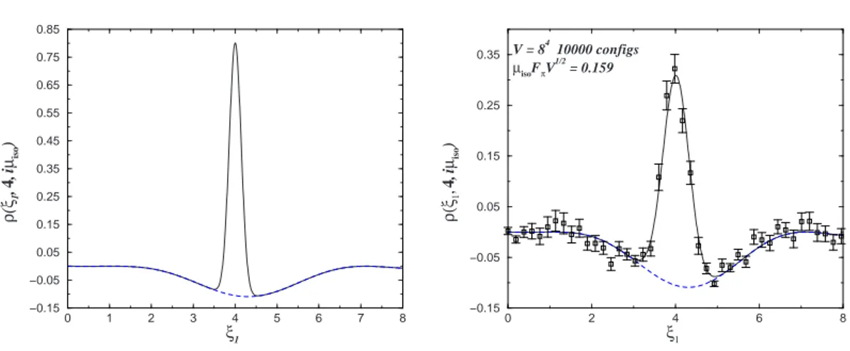
The interest in the real isospin potential lies in the fact that though the fermion determi-nant remains real and positive (and thus amenable to numerical simulations), the eigenvalues of the single quarks acquire a non-vanishing imaginary part breaking the hermiticity of the Dirac operator; this feature resembles the real chemical potential theory [32, 33, 34]. On the contrary, it could seems strange but what makes the imaginary chemical potential QCD an interesting theory is that it is not like the real chemical potential theory: imaginary isospin does not alter the hermiticity of the Dirac operator itself, and, as a consequence, it can be used as a parameter deforming the real Dirac operator spectra. As an example we show picture 1.2 where the introduction of an imaginary isospin chemical potential alters the spectral 2-points correlation function spreading the δ function contribution arising at equal points; this approach has been recently used to give a direct measurement of the pion decay constant Fπ from the spectrum [27, 35, 36, 37, 38, 39].

1.3 Random Matrix Theory

1.3.1 A brief introduction to RMT

Random Matrix Theory (RMT) is nothing but a powerful tool used to describe some specific

properties of complex or chaotic systems.

RMT describes ensembles of matrices with random numbers as matrix elements, in par-ticular distributions and correlations of the eigenvalues of these matrices are usually com-puted when their dimensions approach infinity. The set of the possible matrix ensembles is rather small7 _{and the choice of the proper one is done simply checking the symmetries of}

the system to be described. For many simple problems the description is possible through the use of a single random matrix [44, 45], in some cases it may be useful to consider RMT

(22)

0 1 2 3 4 5 6 7 8 ξ1 −0.15 −0.05 0.05 0.15 0.25 0.35 0.45 0.55 0.65 0.75 0.85 ρ ( ξ1 , 4, i µiso ) 0 2 4 6 8 ξ1 −0.15 −0.05 0.05 0.15 0.25 0.35 ρ(ξ 1 , 4, i µiso ) V = 84 10000 configs µ_isoF_πV1/2 = 0.159

Figure 1.2: On the left hand side we show the two point correlation function ρ(ξ1, ξ2) with one

eigenvalue fixed at ξ2= 4, for for zero (dashed) and non zero isospin potential (full). The δ-function

peak at ξ1= ξ2 for µisohas not been shown. On the other side we show the two point correlation

function at fixed ξ2= 4 measured on a 84 lattice. Pictures taken from [27].

with two or more random matrices [9, 46, 47]. The main value of these theories is that in many cases they are integrable systems and in most of them the computation are relatively easy, and, more importantly, have already been done analytically.

As said above RMT is a tool, and every tool has limitations: the strongest one (that from some point of view is a value too) is that RMTs depend on really few external (physical) parameters, in most cases it is just one (like in χRMT where the only input is the chiral condensate Σ): they can be used only to describe either simple systems or systems in particular regimes where all the relevant dependences are on few (one or two) physical parameters.

Despite these strong limitations, RMT has been applied in many different fields: excited states of heavy nuclei8_{, complex molecules, transport properties of mesoscopic systems,}

two dimensional gravity, conformal field theory, growth problem, non-trivial zeros of the Riemann ζ function and, obviously, QCD. An important conjecture9 _{providing criteria of}

applicability of RMT was provided by Bohigas Giannoni and Schmidt [49]10_{: their claim is}

that the spectra of systems whose classical analogues are ergodic chaotic systems show the same fluctuation properties as the proper RMT. A good review on the history and on the applications of RMT can be found in [45].

We will not get into the details of the classification of RMTs here, we will just cite the

8_{Originally, RMT was designed by Wigner to deal with the statistics of eigenvalues of complex manybody}

quantum systems, having in mind the particular case of the scattering of neutrons with heavy nuclei. This application of RMT may be seen as a formal implementation of Bohrs compound nucleus hypothesis.

9_{Altough a formal proof has not yet been provided remarkable progress in that direction has been made,}

see [48].

(23)

1.3. RANDOM MATRIX THEORY

most important theories introduced by Wigner and Dyson: a) the first one introduced is the ensemble of Hermitian matrices with real, complex and quaternion numbers, respectively known as orthogonal ensemble (OE or, according to the Dyson classification, β = 1), unitary ensemble (UE or β = 2) and symplectic ensemble (SE or β = 4); b) the second set introduced is the one of unitary matrices with real, complex and quaternion numbers, known as circular orthogonal ensemble (COE) and so on. In the present work we will not deal with any of these classical ensemble, we will focus on an implementation of the unitary ensemble taking into account the chiral structure (called chiral unitary ensemble, χUE) introduced by Shuryak and Verbaarschot [5] to describe the properties of the Dirac operator of QCD. We mention that χRMT may be defined for real and quaternion numbers [6, 19] giving rise to effective theories describing 2-colour QCD (χOE) and QCD with quarks in the adjoint representation (χSE).

Concerning the classification of RMTs we have focused the attention only on the matrix sets without taking in account the weight function. The reason for this choice lies in the fact that there is strong evidence, and in some cases there are proofs too (see [45]), of the independence from the infinite matrix dimension limit on the particular choice of the weight function (under some broad hypotheses). This property is usually referred to as RMT universality and justifies the usual simple choice of the gaussian weight function.

The problem of RMT universality is currently being studied in mathematical literature, see [51].

1.3.2 Chiral Random Matrix Theory

Chiral Random Matrix Theory (χRMT) was first introduced in [5] for QCD with 3 or more

colours and quarks in the fundamental representation (this model is usually referred to as

χUE). The theory was derived starting only from the symmetries of the Dirac operator and

from its topological structure. We will briefly summarise this procedure. The starting point is the Dirac operator in the gauge field Aν:

iD ≡ iγνDν = iγν∂ν+ γνAν. (1.44)

Its chiral symmetry {iD, γ5} = 0 implies that the eigenvalues will occur in pairs ±λ apart

from zero eigenvalues. The last relation forces the eigenfunctions of the Dirac operator φλ

to be related by the property φ−λ = γ5φλ. The number of zero eigenvalues is fixed by the

Atiyah-Singer index theorem and is equal to the winding number ν. Let us consider a finite volume discretized theory, one can turn to a chiral basis ψL,k, ψR,k with γ5ψR,k= ψR,kand

γ5ψL,k= −ψL,k. Zero eigenvalues may be either right handed or left handed. In this chiral

basis expansion the massless action becomes: Z d4_{x ψ iDψ =}X k,l Ã χ∗ R,k χ∗ L,k ! Ã 0 iDLR iDRL 0 ! Ã χR,l χL,l ! (1.45)

(24)

where χS,k are the coefficients of the expansion of the field ψ in the chiral basis ψ =

P

kχR,kψR,k+ χL,kψL,k and the matrix elements are given by

DLR,kl=

Z

d4x ψR,k∗ D ψL,l (1.46)

and from the anti-hermiticity11_{of the euclidean Dirac operator D}

RL= DLR† . The functions

φ are the eigenfunctions of of the Dirac operator for a given configuration A, and only for

that configuration the matrix DLR is diagonal; for all the other configurations it will be a

rectangular matrix with a dimension exceeding the other of ν (due to the presence of ν zero eigenvalues of the Dirac operator). Let us say we have N− left-handed eigenfunctions and

N+= N−+ ν right-handed ones.

The ones above are just algebraic manipulations, and the key observations have still to be been done. We know from other approaches (χPT) that there are properties of QCD only resulting from the chiral structure and from overall symmetries (like the Leutwyler-Smilga sum rules, see sect. 1.1.3), disregarding the particular dynamics of the theory; starting from this wisdom the main idea is that whenever we are only interested in these properties we can substitute the Yang-Mills action, that is a weight-function for the matrix DLR,

with a simpler weight function with the same structure satisfying the same symmetries but disregarding the microscopical QCD dynamic:

³

DLR,kl[Aµ], eSY M[Aµ]

´

→ (Tkl, w(T )) (1.47)

where T is a N+× N−rectangular complex matrix12. The simplest choice possible for the

weight function is the one of a gaussian wight-function

w(T ) = Exp£−σN T r£T†_T¤¤ _(1.48)

where the quantity σ is a dimensionless free parameter (the only parameter in the theory) and the factor N = N++ N− has been introduced due to a useful convention. The simple

gaussian choice for the wight function is supported by results assuring that, according to reasonable hypotheses, the N → ∞ limit is independent of the particular choice of the weight function [52, 53, 54].

The substitution above is expected to be valid only for investigating the energy spectrum in given conditions, conditions which, we already know from different ways, ensure that the spectrum can be studied by means of “universal” effective theories [5]: in our case it is valid

11_{The possible presence of anti-unitary symmetry may imply that the matrix D}

LRis a real or quaternion matrix. If such a symmetry is absent the matrix is a complex one.

12_{If one considers the elements of T real number or quaternions one obtains chOE and chSE}

respec-tively. These theories may be used to describe properties of QCD-like theories with additional anti-unitary symmetries.

(25)

only when considering the ε-regime. The resulting RMT is: Z dT e−σN T r[T T†] Nf Y f =1 Det " mf1N+ iT iT† _m f1N− # . (1.49)

This model take the name of chGUE.

Naively speaking the argument above can be summarised saying: there are quantities, like the Leutwyler-Smilga sum rules, that are functions of the lower part of the spectra, which does not depend on the particular QCD dynamic but only on the symmetries hence they are universal; since they are universal they can be described by any theory with the same symmetries. This one may seem to the reader a rash conclusion, a conjecture rather than an argument, and in fact it is a conjecture. When it was formulated in [5] it was introduced together with an explicit computations showing that it was possible to obtain the very same Leutwyler-Smilga sum rules as χPT starting from χRMT. This was a strong argument in favour of the conjectured equivalence but was not at all explaining why QCD should show some universality feature13_.

A subtle argument in favour of the universality was proposed in [55] where it is shown that under well accepted hypotheses (like the pion-pole dominance, the Gell-Mann-Oaks-Renner relation or semiclassical arguments), if one considers the eigenvalues of the 4-dimensional Dirac operator like the eigenvalues of a quantum Hamiltonian in a 4+1 dimensional theory an ergodic dynamic in this additional (Schwinger) time it follows from the ε-regime range energy of 4-dimensional QCD14_{. This result, together with the Bohigas-Giannoni-Schmidt}

conjecture [49], gives an explanation too of the equivalence between χPT and χRMT: spectra of classically ergodic chaotic systems may be described through “proper” random matrices. The “proper” one for this particular case has to be chosen in order to verify the same symmetries and topological structure as QCD and, hence, it is the one in eq. 1.49.

Here we will not show details that can be found in [55], its easier and impressive to show some numerical results where comparison between the spectrum obtained by lattice QCD simulations and the one predicted by RMT is made.

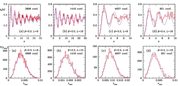
The picture in fig. 1.3, taken from [56], “provides direct evidence for the conjecture” above. Simulations were in 2-colour quenched QCD using the staggered Dirac operator and the comparison was done with χGSE15_{predictions in [57].}

Nowadays the fact that RMT may be used to describe the low energy spectra of QCD in the ε-regime is widely accepted, no matter that a real proof showing how RMT descends directly from QCD is still lacking. In this work we will not fill this gap (deriving low energy

13_{In the same paper the sum rules very verified for an instanton liquid model with the same symmetries.} 14_{The same Schwinger time approach was used in [15] to derive pq-χPT starting from stochastic QCD-like}

theory.

15_{Two colour QCD has an anti-unitary symmetry, its universality class may be χGSE or χGOE according}

(26)

Figure 1.3: QCD spectrum (upper line) and first eigenvalue distribution (lower) from lattice

sim-ulations and RMT predictions at different gauge couplings β and lattice volume L4_{. Picture taken}

from [56].

properties from microscopical QCD is really an ambitious task!), but we will prove the existence of a mathematical link with the well accepted χPT.

1.3.3 An example: chGUE

In order to understand how RMT works it may be instructive to show an explicit com-putation as an example; we compute here the spectral correlation function for the chGUE with Nf dynamical fermions like in eq. (1.49). For simplicity we show the computation for

zero topological charge as it was shown for the first time in [58]. The starting point is that any complex matrix T can be diagonalised according to T = V · Λ · W , with V ∈ U (N ),

W ∈ U (N )/U (1)N _{and Λ is a positive definite diagonal matrix with entries λ}

1, . . . , λN.

The measure transforms according to

dT = dµ(U ) dµ(W )Y i dλi Y k<l (λ2 k− λ2l)2 Y k λk. (1.50)

The measures over the unitary matrices dµ(U ), dµ(W ) are Haar measures and the integra-tion gives a trivial contribuintegra-tion since these angular degrees of freedom decouple from the rest of integral.

The N-eigenvalue distribution, also called joint probability density function (jpdf) is given by: ρN(λ1, . . . , λN) = Y k<l (λ2k− λ2l)2 N Y k=1  λk Nf Y f (m2f+ λ2k)   Exp " −2σN N X k=1 λ2k # . (1.51)

(27)

The spectral density function (or any k-point correlation function) can be obtained in-tegrating the jpdf over the remaining N − 1 (N − k) eigenvalues. The technical tool used to solve this integration is provided by the orthogonal polynomials [44]: one defines a scalar product in a function space, in this case:

< f, g >= Z dλ2 Nf Y f (λ2_{+ m}2 f)e−2σN λ 2 f (λ) g(λ). (1.52)

Orthogonal polynomials are obtained performing Gram-Schmidt orthogonalisation to the monomials λ2j_{, j ∈ N. The term}Q

k<l(λ2k− λ2l) is written as a Vandermonde determinant

and this determinant is expanded using the Cramer’s rule, but instead of writing λ2j_k one can consider any monic Pj(λ2k). All the terms involving integrated variables can be integrated

using the orthogonalisation relation < Pk, Ps >= rkδk,s. The result is a sum of Pk · Pk.

This sum can be performed through the Christoffel-Darboux formula. For mf = 0 the

polynomials are known16_{, they can be written in terms of Laguerre polynomials L}b

a and the

result for the spectral density function is:

ρ1(λ) = 2σN N ! (N + Nf− 1)! (2σN λ2₎Nf+1/2_Exp£_{−2σN λ}2¤ _(1.53) × ³ LNf N −1(2σN λ2)L Nf+1 N −1 (2σN λ2) − L Nf N (2σN λ2)L Nf+1 N −2 (2σN λ2) ´

Rather than in the quantity above, we are interested in its microscopic limit ρs, that

is N → ∞ limit keeping x = 2N λ constant. The reason for this interest lies in the fact that this limit is not sensitive to the particular choice of the weight function (restricted to a broad class of function) [52, 53, 54] and, obviously, is the one that is believed to describe QCD spectrum. The quantity to be kept fixed, σ N λ, strongly reminds the quantity Σ V λ in the Leutwyler-Smilga sum rule (1.21), where σ plays the role of the chiral condensate Σ and the number of eigenvalues N is related to the volume V . The microscopic limit of (1.53) can be obtained using the limit:

lim N →∞ 1 NαL α N ³ y N ´ = y−α/2_J α(2√y) (1.54)

where J is a Bessel function of the first kind. The result is

ρs(x) = σx ³ J2 Nf ³√ 2σx´− JNf+1 ³√ 2σx´JNf+1 ³√ 2σx´´. (1.55) The same result was obtained later in [60] starting from χPT and was confirmed through lattice simulations in [61]. The explicit result for the k-point correlation function can be found in [52].

The mf 6= 0 explicit solution can be read off from [54, 59]. Looking at eq. (1.51), and

considering that z2_{+ m}2

f = (z + imf)(z − imf), one can see that any flavour can be treated

16_{They are also known for m}

(28)

as an additional imaginary eigenvalue (modulo some easy to calculate mass-dependent pref-actor). After this remark we see that the microscopic limit has to be considered scaling the quark masses keeping m · N fixed. The analogous of this condition in χPT is that we are considering only quantities depending on the masses scaling like ε0_{, see sect. 1.1.3.}

1.3.4 Non Hermitian chiral RMT

RMTs may be used to describe non Hermitian theories too. We consider here only the case relevant to the purposes of this work, that is the chiral case used to describe low energy properties of QCD with a chemical potential (see [62] for a review). The latter is a theory whose Dirac operator is no more Hermitian, and it can be approached with the very same idea used in the Hermitian cases; an equivalent of the “heuristic” substitution of eq. (1.47) may be provided: ÃÃ 0 iDLR[A] + µ iDRL[A] + µ 0 ! , eSY M[A] ! → (DRM T, w(DRM T)) (1.56)

where this time DRM T is a non-Hermitian matrix.

Two different matrix structures have been introduced for DRM T, the first by Stephanov

[8] which consists of adding a Hermitian constant term (miming the chemical potential) to the standard anti-Hermitian random matrix part (Dirac operator), in formulas:

Ã 0 iDLR[A] + µ iDRL[A] + µ 0 ! → Ã 0 i T + µ i T†_{+ µ} ₀ ! . (1.57)

The other model was introduced by Osborn [9] and consists of two independent random matrix parts, one Hermitian and one anti-Hermitian:

Ã 0 iDLR[A] + µ iDRL[A] + µ 0 ! → Ã 0 i T + µ W i T†_{+ µ W}† ₀ ! . (1.58)

In both models the quantity µ is a dimensionless parameter (< 1) playing the role of the chemical potential. The usual choice for the random matrix weight function is the gaussian one.

Despite the fact that Osborn’s model is a two matrix model and that doubling the number of variables may seem to be increasing the complexity of calculations this is not always the case, there are quantities, like the spectral density function [9], whose computation in this framework is much easier than in the other one [63]. On the other side Stephanov’s model is more efficient in other computations (like the study of QCD phase diagrams, e.g. see [64]). Every time computations (or simulations) have been performed in the two models they were in agreement in the thermodynamic limit ([65, 9, 63, 66]). These two models are completely equivalent and in chapter 4 we will give a mathematical proof of it.

(29)

The partition functions for the two models are (N+≥ N−)

Z = Z dT e−σN T r[T T†_] Nf Y f =1 Det " mf1N+ iT + µ1N− iT†_{+ µ1} N− mf1N− # (1.59)

(the off diagonal parts are N+×N−matrices, and the identity matrix 1N−has to be intended

like the biggest identity matrix fitting in this rectangular) for Stephanov’s model and

Z = Z dT dW e−σN T r[T T†_{+W W}†_] Nf Y f =1 Det " mf1N+ iT + µW iT†_{+ µW}† _m f1N− # (1.60)

for Osborn’s one.

We briefly mention the way used by Osborn to solve his model, it is not different con-ceptually from the one sketched in sect. 1.3.3 for the Hermitian model. The starting point is to note that the blocks of the Dirac operator can be simultaneously “triangularised”17

iT + µW = U (X + R)V

iT†+ µW† = V†(X + R)U† (1.61)

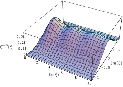
and that the upper triangular parts V and R are irrelevant both to the Jacobian of this triangularisation and to the argument of the integration. As a consequence it is possible to express the integrals in terms of the (diagonal) elements of X and Y , or even better, just of the complex (diagonal) elements of X · Y . Once obtained for the N -eigenvalues distribution an analogous of eq. (1.51) in order to obtain the k-point function one integrates the remaining N −k complex variables through the complex-orthogonal polynomials method [67, 68, 69]. Conceptually it is not different from the real one already encountered in the previous section, the only difference lies in the fact that the integration defining the scalar product is over the whole complex plane. An explicit solution can be written in terms of Laguerre polynomials for finite N and its N -infinite limit in terms of Bessel functions. Showing a picture of the typical density function is more clarifying than writing the explicit expression (for that we refer to [9, 62]), see fig. 1.4.

In the previous section we have pointed that the N → ∞ limit can be written only when the mass changes with N like N−1_{. An analogous of this scaling property exists for}

the “chemical potential” too: N · µ2_{has to be kept fixed. This is usually called weak}

non-hermiticity limit, in order to distinguish it from the strong one where µ2 _{stays finite (see}

[70] for an overview on the topic). The weak non-hermiticity limit is the RMT equivalent of the power counting (1.42) in χPT.

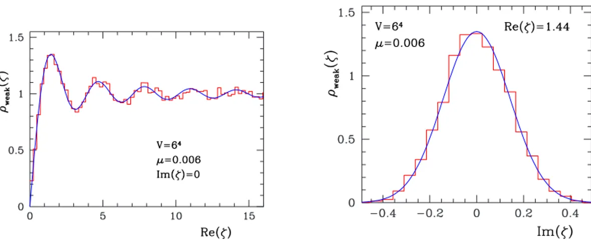
The quenched spectrum predicted by this model18 _{has been checked with the one}

ob-tained from lattice simulations [72, 73] showing a good agreement between the data (see fig.

17_{The block are not square matrices due to the topological charge.}

18_{Strictly speaking the model was not this one, it was an older eigenvalues-model introduced by Akemann}

[68] having the same m · N → 0 as Osborn’s one. This model was not introduced starting from a matrix model.

(30)

0 2 4 6 8 10 -1 -0.5 0 0.5 1 0 0.1 0.2 0.3 0 2 4 6 8 10 Re(ξ) Im(ξ) ρν=0 s (ξ)

Figure 1.4: The quenched spectral density for non-zero chemical potential for zero topological charge. Picture taken from [62].

1.5).

What we have shown up to this point is the non-Hermitian chUE, but exactly like UE and chUE, non-Hermitian chiral RMT (sometimes referred to as χR2MT) has a orthogonal and symplectic partner too, whether one considers random matrices with real or quaternionic entries. These two models are particularly interesting since they describe QCD-like theories that can be simulated on the lattice. In [74] the predictions for the symplectic ensemble [69, 71] have been successfully compared with the lattice data coming from 2-colour QCD with staggered fermions at non-zero chemical potential.

1.3.5 Isospin chemical potential RMT

As in QCD the chemical potential matrix may be chosen not proportional to the identity. In general we can define the Dirac operator for a quark with mass mf and chemical potential

µf, it is given by [75]: iDf+ mf ≡ Ã mf1N+ iA + µfB iA†_{+ µ} fB† mf1N− ! , (1.62)

the partition function is:

Zpq = *_n f Y f Det [iDf+ mf] + (1.63) = Z dA dB e−σN T r[AA†_+BB†_] nf Y f Det " mf1N+ iA + µfB iA†_{+ µ} fB† mf1N− #

(31)

1.4. PARTIALLY QUENCHED QCD AND SUPERANALYSIS

Figure 1.5: Density of small Dirac eigenvalues of a 64 _{lattice at non-zero chemical potential, cut}

along the real axis (left) and parallel to the imaginary axis at the first maximum (right). The histogram represents lattice data, and the solid curve is theoretical prediction. Picture taken from [72].

where A and B are complex N+× N− random matrices with Gaussian weights, and, as in

eq. (1.49) the measures dA and dB are the flat measure in the independent entries of the matrices.

This model was introduced and solved for isospin chemical potential19_{for real case in [66]}

(it follows as a particular case of [9]) and imaginary20_{one in [75]. These models are defined}

following Osborn’s prescription [9]: the chemical potential term is a coupling between two random matrices; this is just an apparent complication indeed this introduction makes the model simpler: for two different chemical potentials one can go to an eigenvalue basis and use bi-orthogonal polynomials.

The properties making these two isospin theories interesting have been already sum-marised in section 1.2, an example of the results obtained is the Fπ-depending deformation

of the two point correlation function in fig 1.2.

The issue of universality is more subtle here because the matrices A and B will couple after changing variables. We refer to [75] for a more detailed discussion.

1.4 Partially quenched QCD and superanalysis

We will introduce here an important instrument for deriving the properties of the spectrum of an operator: the resolvent method. This is a general method that can be applied both to QCD and to RMT, though in the latter case it is inconvenient compared to the simpler orthogonal polynomial method. It leads to the introduction of a QCD-like theory with

19_{The chemical potential values are coupled in +µ and −µ.} 20_{In this case the solution given holds for N}

Effective theories of finite volume QCD

University of Pisa

Graduate Course in Physics

School of Graduate Studies in Basic Sciences “Galileo Galilei”

Brunel University West London

Department of Mathematical Sciences

Ph.D. thesis:

“E

FFECTIVE THEORIES

OF FINITE VOLUME

QCD”

Candidate:

Francesco Basile

Supervisors:

Prof. G. Akemann

, Brunel University

Abstract

Contents

Chapter 1

Introduction

A

1.1

Chiral Perturbation Theory

1.1.1

The chiral Lagrangian

1.1.2

Finite volume χPT and the ² regime

1.1.3

Chiral Perturbation Theory at O(ε

)

1.1.4

Chiral Perturbation Theory at O(ε

)

1.2

Non-zero chemical potential

1.3

Random Matrix Theory

1.3.1

A brief introduction to RMT

1.3.2

Chiral Random Matrix Theory

1.3.3

An example: chGUE

1.3.4

Non Hermitian chiral RMT

1.3.5

Isospin chemical potential RMT

1.4

Partially quenched QCD and superanalysis

₎

₎