The information content of M3 for future inflation in the euro area

(1)

The Information Content of M3

for Future Inflation in the Euro Area

By

Carmine Trecroci and Juan Luis Vega

C o n t e n t s : I. Introduction. - II. Investigating the Leading Indicator Properties of M3 in a Money Demand VAR System. - III. Leading Indicator Properties of M3 within an Extended Framework. - IV. Encompassing Rival Models. - V. Conclusions.

I. Introduction

T

here are good theoretical reasons - namely the claim that inflation is ultimately a monetary phenomenon - for underlying the

specialness

of monetary aggregates among the set of variables which are closely monitored by central banks. This relationship between money growth and inflation is present in almost every well-articulated economic model, thereby warranting, on its own, that money be given a prominent role in the conduct of monetary policy.

At a more practical level, economic theory also suggests a number of possibilities for implementing a prominent role for money within a monetary policy strategy aimed at price stability. Firstly, monetary aggregates may play a nominal-anchor role, whereby the announcement of a reference for money growth well into the future help economic agents to form expectations about prices. This function entails quite a few practical requirements: (i) a relationship between money and prices must exist, be reasonably stable (predictable) and be invariant to central bank's own actions (i.e., be structural in the sense of being immune to the Lucas critique);

(ii)

the announcement must be credible, implying commitment on the part of the central bank and requiring in turn

Remark: This research was carried out while the first author was at the ECB as part of

the Research Graduate Programme run by the Directorate General Research, and a Re- search Fellow for the University of Glasgow, Department of Economics. We wish to thank I. Angeloni, J. Darby, V. Gaspar, S. Gerlach, J. Malley, A. Muscatelli, R. Mac- Donald, A. H. Meltzer, R. Sandilands, E Smets, E Spinelli, J. Stock, L. E. O. Svens- son, S. Wren-Lewis and U. Woitek for comments on earlier drafts. This work has also benefited from comments of members of the ECB Working Group on Econometric Mod- elling as well as seminar participants at the ECB, the Universities of Glasgow, Brescia, Bari and Strathclyde. The usual disclaimer applies.

(2)

Trecroci/Vega: The Information Content of M3 23 that the m o n e y stock is controllable at some time horizon by means o f the instruments available to the central bank (typically, a short-term interest rate). F o r the euro area, there exists some empirical e v i d e n c e that broad m o n e y M3 m a y not be controllable at short-term horizons, precluding a pure m o n e t a r y targeting strategy. H o w e v e r , available em- pirical e v i d e n c e also points to both (i) and (ii) being fulfilled at medi- u m - t e r m horizons by M3 (see C o e n e n and Vega 2001 and the references therein). This observation was indeed the main empirical basis for the selection o f this aggregate when the first m e d i u m - t e r m reference value for M3 m o n e y growth was a n n o u n c e d by the G o v e r n i n g Council o f the E u r o p e a n Central Bank in D e c e m b e r 1998.1

M o n e y m a y also play a role within the strategy as an information variable to be included within the set o f indicators which are regularly r e v i e w e d in the assessment o f the outlook for, and risks to, price stability. This function entails one practical requirement, n a m e l y that past and current m o n e t a r y d e v e l o p m e n t s contain valuable information about future prices, i.e., m o n e y being a leading indicator for inflation. 2

F r o m an empirical viewpoint, the investigation o f leading indicator properties o f m o n e y can be c o n d u c t e d by following two different (but not incompatible) strategies. On the one hand, a structural model o f the e c o n o m y can be estimated and, subsequently, the indicator properties o f m o n e y can be directly inferred from the restricted r e d u c e d f o r m o f the model. Alternatively, the indicator properties o f m o n e t a r y aggregates can be investigated straight from the unrestricted r e d u c e d form o f the m o d e l itself by means, for instance, o f w e l l - k n o w n G r a n g e r non- causality tests. T h e latter is the most c o m m o n approach in the literature but a n u m b e r o f serious concerns need to be borne in mind.

First, the c o n c e p t o f G r a n g e r causality refers to the entire universe o f information (the c o m p l e t e v e c t o r o f variables which characterizes an

l See ECB (1999). Issing et al. (2001) discuss the analytical foundations of the monetary policy strategy of the ECB.

2 At the conceptual level, the two roles for money - nominal anchor and leading indi- cator - need to be distinguished. The first is about whether knowledge of future mone- tary developments (the central bank announcement) help economic agents to predict inflation. The second is about whether past monetary developments help predict infla- tion, which is neither necessary nor sufficient for the first. Indeed, as shown in Sims (1972), the necessary and sufficient condition for the first is the existence of Granger causality from prices to money. This direction of causality is implied by the results reported in Coenen and Vega (2001). Also note that this view contrasts with the starting point in EstreUa and Mishkin (1997), who maintain that in all potential uses of monetary aggregates "it is necessary first and foremost that the aggregates have some values as information variables".

(3)

24 W e l t w i r t s c h a f t l i c h e s A r c h i v 2002, Vol. 138 (1)

economy) and, therefore, is intrinsically not operational. On the other hand, practical applications are necessarily confined to limited information sets (sometimes quite limited due to the lack of degrees of free- dom frequently available to the applied researcher). In this context, there is no guarantee that inference does not change with the information set under consideration. 3 This observation strongly warns against conclusions drawn from reduced forms that are unlikely to be derived from a minimally well-specified structural model. In this respect, Woodford (1994: 101) noted - as Granger (1988) did too - that this problem may be particularly acute when dealing with policy-related variables: "... the mere fact that an indicator is found not to enter significantly in an inflation forecasting regression does not necessarily mean that" the central bank "... should be advised not to pay any attention to that variable. For the absence of forecasting power might simply imply that the variable is already being used..." by the central bank "in making policy, and in approximately the right way..."

And second, identifying which characteristics of the transmission mechanism account for stylized facts documented via the estimation of a reduced form is most crucial if any empirical finding concerning indicator properties of money were to be used in policy. Otherwise, when structural interpretations are absent, one would need to conclude with Woodford (1994: 102): "...the mere fact that an indicator is found to be useful in forecasting inflation does not tell much about the desirability of a policy that involves feedback from that indicator ... the ability of the indicator to signal the underlying sources of inflationary pressures that one wants to respond to may be impaired by the very fact that the monetary authority responds to it."

With these limitations in mind, the paper proceeds as follows. First, in Section II leading indicator properties of broad money M3 are analyzed by conducting standard tests that money does not Granger-cause prices in the context of a cointegrated VAR system that has recently been proposed to investigate money demand in the euro area. In Sec- tion III, we extend this empirical framework to look into the recent claim that - in the context of a P-star model - the real money gap (i.e., the gap between current real balances and long-run equilibrium real balances) has substantial predictive power for future inflation in the euro area. Finally, in Section IV we conduct a number of encompassing tests to compare the model developed in the previous section with

3 By contrast, cointegration is a property which is invariant to expansions of the information set.

(4)

Trecroci/Vega: The Information Content of M3 25 a competing structural model of inflation where no explicit role is given to monetary developments. In Section V, some tentative conclusions are drawn.

Our results illustrate the claim above that inference about Granger non-causality may vary with the information set at hand and confirm the findings that a significant positive association exists between the real money gap and future inflation up to five to six quarters ahead, reaching a maximum at the three-to-four quarter horizon. It is also shown that, although the extended P-star model outperforms the structural model in terms of out-of-sample forecast accuracy at horizons above two quarters, the hypothesis that no useful information is contained in rival evidence can be rejected at standard confidence levels. We conclude that each model appears to have strengths of its own: both of them incorporate some information which turns out to be relevant to explain GDP inflation at different horizons; both of them, however, also fail to provide, on an individual basis, a complete account of inflation developments in the euro area.

II. Investigating the Leading Indicator Properties of M3 in a Money Demand VAR System

Following Coenen and Vega (2001) [CV henceforth], let Z ' = ( m - p , ~, y, R s, R t) = ( m - p, :~, X ' ) be a vector of CI(1,1) variables consisting of real holdings of M3, (m - p), the inflation rate (as measured by the annualized quarterly changes in the GDP deflator, :~ = 4Ap), real GDP, y, and the short- (R s) and long-term (R l) interest rates. Consider the following VAR model:

k

Z t = ~ Ji)Zt_ i -FV t

(2.1)

i=l

and its VECM representation:

k-I

A Z t = ~ Ai) Azt_i + I " A ' Z t _ 1 + V t (2.2)

i=l

with 1" and A (5, r) full-rank matrices of loading coefficients and cointegrating relationships, respectively.

Model (2.2) with lag length k = 2 and cointegration rank r = 3 was estimated in CV. In the present context, leading indicator properties of broad money M3 can be investigated by conducting tests that money

(5)

26 Weltwirtschaftliches Archiv 2002, Vol. 138 (1)

does not Granger-cause prices, following the results in Toda and Phillips (1993, 1994a, 1994b). We define the following partitioned matrices:

mt - Pt 1

z,=!

/;

~ S t )

G = F2 and

r3

(A~I A[~ A~

Ai)= [A~] Ai~)

2 A~)3

~A~ A~)2 A~

I A1 )

A = A 2 .

~,a3 )

i=1 ... k - I ; (2.3)

Toda and Phillips (1993,1994a, 1994b) suggest some operational pro- cedures for conducting Granger causality tests that are applicable in the case of testing the causal effects of one variable on another group of variables and vice versa. In particular, three sequential causality Wald- type tests are recommended:

if H2 ts rejected, test H*

(P1)

Test H i \otherwise," test H•

if H~ is rejected, test H*

(P2)

Test H~ \otherwise, test H~

l ifHl is rejected, reject the null*

/ if both are rejected, test

/ H~! ifr

> 1,

or reject the

(P3)

Test HI*

otherwise, test ~ null if r = 1 otherwise,

H~ and H~

\ accept the null of non-

\ causality

where the different hypotheses are defined as follows (see Toda and Phillips (1993) for the asymptotic distributions of the corresponding Wald tests):

H*: All . . . A~l 1 = 0 and

I'2A ~

= 0 (short- and long-run causality)

H_~: All . . . A~T 1 = 0 (short-run causality)

H~': A1 = 0 (long-run exclusion)

H~': F 2 = 0 (weak exogeneity)

(6)

Trecroci/Vega: The Information Content of M3 27 The estimation of model (2.2) over the sample period 1980:Q1- 1998:Q4 yields the following results (p-values in brackets): H*: 222 = 0.251 (0.882); H~*: ~ = 0.069 (0.793); H~': ~3 = 12.72 (0.005); H~: ~3 = 26.43 (0.000); n~'t: ~ = 0.251 (0.617).

Therefore, on the basis of the Toda and Phillips tests conducted above, the null hypothesis that M3 money does not Granger-cause GDP prices within the information set at hand cannot be rejected at standard confidence levels. This inference appears to be robust to the chosen sample period. When the VAR is estimated recursively over the sample 1993:Q1 - 1998:Q4, the maximal test statistics for the hypotheses H*, H• and H~'t are: 0.477, 0.268 and 0.937, respectively. All of them are well below the corresponding Z z critical values. 4 The same results hold when the estimation sample starts in 1985, dropping the first five years from the analysis.

One weakness of the Phillips-Toda tests conducted above is the fact that they rely on pre-tests for unit roots and cointegration. Accurate de- termination of the number of unit roots and cointegration rank in small samples may be problematic, leading to pre-test biases in Granger causality tests conditioned on the estimation of these parameters (see Yama- da and Toda 1998). Against this background, we investigate in the following whether the failure to reject Granger non-causality of m on p could be attributed to mis-specifications of the cointegration rank and/or the degree of integration of the variables included in the CV money demand system.

To this end, we follow Toda and Yamamoto (1995) 5. These authors show how levels VARs can be estimated and general restriction be tested even if the time series involved are integrated or cointegrated of an arbitrary order. Firstly, a usual lag selection procedure can be applied to determine the lag length (k*) in the VAR. Secondly, a (k* + dmax) th-order VAR can be estimated, where dma x is the maximal order of integration suspected to occur among the variables in the system (typically 1 or 2). Thirdly, disregarding the last dmax lagged terms, general restrictions on the first k* coefficient matrices can be tested for using standard (asymptotic) inference.

In Table 1 (left panel) the suggestions in Toda and Yamamoto (1995) are used to test for Granger non-causality of m on p in VARs com-

4 It should be noted that the use o f x 2 critical values in this recursive context biases results towards rejection of non-causality, since no allowance is made for the endogenous search. In this sense, the conservative nature of the exercise should provide a strong indication that the conclusion on non-Granger causality is firmly grounded.

(7)

Table 1: Tests for Granger Non-Causality of M3 on Prices in the VAR( k )

Granger non-causality tests for Wald tests for M I : (m,p,y, s, l) M2: H0:M2 vs Hi: M1

( m - p , y, s, I, p)

I(2) model I(1) model I(1) model I(2) model I(1) model dmax = 2 dmax = 1 dmax = 1 dmax = 2 dmax = 1

(1) (2) (3) (4) (5) i i k = l 0.110 0.970 0.384 9.109 19.490 (0.740) (0.325) (0.535) (0.105) (0.109) k = 2 0.579 0.793 0.958 13.255 9.837 (0.749) (0.673) (0.619) (0.151 ) (0.364) k = 3 1.102 0.633 1.066 19.607 20.599 (0.777) (0.889) (0.785) (0.106) (0.245)

Note." The VARs include two set of variables: Z l = (m, p, y, R s, R t) and Z 2 = (m-p, Ap, y, R s, Rt). The maximal order of integration is presumed to be 2 (1(2) model) or 1 (I(1) model) in Z l and 1 (I(1) model) in Z 2. Hence, columns 1 and 2 refer to specification in Z 1 = (m, p, y, R s, R t) under alternative hypotheses on the maximal degree of integration among the variables comprising the system: d~nax = 2 (col. 1) or drnax = l (col. 2). Column 3 refers to specification in Z 2 = (m-p, Ap, y, R s, R z)

under the hypothesis dmax = 1. The right panel reports tests for model reduction from M1 to M2. Finally, the V~,R's lag length are set to k = 2 in the second row. Howev- er, possible mis-specifications of k are accounted for by reporting also results for k* + 1 and k * - 1.

prising two set of variables: Z t = (m, p, y, R s, R l) and 2 2 = (m - p , Ap,

y, R s, Rl). The maximal order of integration is presumed to be 2 (I (2) model) or 1 (I(1) model) in Z t and 1 (I(1) model) in Z 2, allowing for the possibility of nominal variables being I (2) but constraining real variables to be, at most, I(1). This is consistent with the findings in CV but encompasses models in which both nominal and real variables are assumed to be I(1). Hence, columns 1 and 2 in Table 1 refer to specification in Z I = (m, p, y, R s, R l) under alternative hypotheses on the maximal degree of integration among the variables comprising the system: dmax = 2 in col. 1 or dmax = 1 in col. 2. Column 3 refers to specification in Z 2= ( m - p, Ap, y, R s, R t) under the hypothesis dma x = 1. The right panel of Table 1 reports tests for model reduction from M 1 to M2; this is a test for long-run homogeneity of money and prices. Final- ly, consistent with the evidence from both sequential F-tests for lag exclusion and information criteria, the VAR's lag length are also set to k = 2. However, possible mis-specifications of k are accounted for by reporting also results for k* + 1 and k* - 1. The complete set of re-

(8)

Trecroci/Vega: T h e Information C o n t e n t o f M3 29

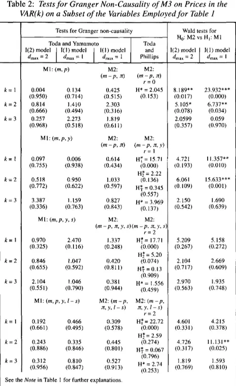
Table 2: Tests f o r Granger Non-Causality o f M3 on Prices in the

VAR(k) on a Subset o f the Variables Employed f o r Table 1

Tests for Granger non-causality Toda and Yamamoto Toda I(2) m o d e l [ l(1)model [ l(1)model and

dma x = 2 dma x --- I dma x = 1 Phillips MI: (m, p) M2: M2: ( m - p , ;r) (mr-P~.rr) , 0.004 0.134 0.425 H* = 2.045 (0.950) (0.714) (0.515) (0.153) 0.814 1.410 2.303 (0.666) (0.494) (0.316) 0.257 2.273 1.819 (0.968) (0.518) (0.611) MI : (m, p, y) M2: M2: (m - p, ~t) (m r ~ l , y) 0.097 0.006 0.614 HT = 15.71 (0,755) (0.938) (0.434) (0.000) H~' = 2.22 0,518 0.950 1.033 (0.136) (0.772) (0.622) (0.597) H~ - 0 345 (0-55'7) 3.387 1.159 0.827 H* = 3.969 (0.336) (0.763) (0.843) (0.137) MI: ( m , p , y , s) M2: M2: (m - p , Jr, y, s)(m - p , ~, y, s'~ r = 2 0.970 2.470 1.337 H~'= 17.71 (0.325) (0.116) (0.248) (0.000) n~' = 5.20 0.846 1.047 0.420 (0.074) (0.655) (0.592) (0.811) H~-= 0.13 (0.909) 2.104 1.046 0.381 H* - 1 556 (0.551) (0.790) (0.944) (0-459) MI: ( m , p , y , l - s) M2: ( m - p , M2: ( m - p , ~ , y , l - s ) & y , l - s ) r = 2 0.192 0.466 0.309 H~'= 22.72 (0.661) (0.495) (0.578) (0.000) H~ = 2.59 0.243 0.335 0.445 (0.274) (0.886) (0.846) (0.801) H~- - 0 067 12 (0779"6) 0.3 0.810 0.527 . , ~ ~, (0.956) (0.847) (0.913) ~0.~;3~" See the Note in Table 1 for further explanations.

Wald tests for H0:M2 VSHl:M1 8.189"* 23.932*** (0.017) (0.000) 5.105" 6.737** (0.078) (0.034) 2.0599 0.059 (0.357) (0.970) 4.72I 11.357"* (0.193) (0.010) 6.061 15.633"** (0.109) (0.001) 2.150 1.690 (0.542) (0.639) 5.209 5.158 (0.267) (0.272) 2.104 2.669 (0.717) (0.609) 2.970 1.935 (0.563) (0.748) 4.601 4.215 (0.331) (0.378) 4.726 11.131'* (0.317) (0.025) 1.819 1.593 (0.769) (0.810) I(2) model ] I(1) model

(9)

suits in the table should permit to assess the robustness of the conclusions based on the Phillips-Toda tests conducted above to different as-

sumptions on maximal order of integration

(dmax)

and the VAR lag

length (k*).

Table 2 reproduces the analysis for different subsets of the variables in the systems: (a) Z 1 = (m, p) and Z 2 = (m - p , Ap); (b) Z 1 = (m, p, y) a n d Z 2 = ( m - p , Ap, y); (c) 1 Zc = (m, p, y, R s) and Z 2 = ( m - p , A p , y, RS);

and (d) Z 1 = (m, p, y, R t - R s) and Z ~ = ( m - p, A p , y, R t - RS). The struc- ture of the table is the same as that of Table 1 except for the inclusion of the corresponding Phillips-Toda tests in column 4.

A number of conclusions can be drawn from the analysis in this section. Firstly, there is little empirical evidence for rejecting Grang- er non-causality of m on p within the information set used in CV. Both the Phillips-Toda tests and the Toda-Yamamoto tests fail to reject Granger non-causality of m on p at standard confidence levels. Sec- ondly, this conclusion, which is stable throughout the sample period, appears to be robust to a number of plausible assumptions concerning: (i) the maximal degree of integration of the variables in the

system; (ii) the lag length selected for the VAR; and, ( i i i ) the imposi-

tion or not of the long-run homogeneity of m and p, though the long- run homogeneity hypothesis cannot be rejected at standard confidence levels. Finally, the results in Table 2 also suggest that the conclusion above is invariant to the reduction of the information set employed in CV.

III. Leading Indicator Properties of M3 within an Extended Framework

1. A P - s t a r M o d e l o f I n f l a t i o n i n t h e E u r o A r e a An attempt to analyze leading indicator properties of M3 within a more 'structural' framework is made in a recent paper by Gerlach and Svens- son (2000) [GS henceforth]. They find that the real money gap (i.e., the gap between current real balances and long-run equilibrium real balances) has substantial predictive power for future inflation in the euro area. They conclude that the real money gap should be an important indicator for the Eurosystem. GS estimate the following P-star type model for the inflation rate: 6

6 See Groeneveld (1998) and the references therein for an overview of the P-star model and for empirical evidence on its relevance for various euro area countries.

(10)

Trecroci/Vega: The Information Content of M3 31

J'ft = a~t_l + Otm (tht_l - th*_l) + Oty (Yt_l - Yt*_l) + F.t ( 3 . 1 a )

~ t - I = (1 - a~) ~t + C~3r ~t-1 (3.1b) ~t = exp (~o + rl t) (3.1c) rh t - ( m - P ) t = ko + k y Y t - ki ( R [ - R t ) (3.1d) A ~ l t = (~0 - f~l [ l ~ l - k 0 - ky y + k i ( R l - RS)]t_l -- I~2 ('71~t -- ~ t ) + ~ 3 A ? n t - 1 "t- U t ( 3 . 1 e ) P * - m t - ko - ky y * + ki ( R l - R~) * (3.1f) rh t - rh* - ( m - P)t - ( m - P * ) t ~ - (t~ -- P * ) = ( m - p ) t - k * - k y y * ; k * = [ k o - k i ( R t - R ' ) * ] , (3.1g) where z(, ~, rfi, and y* stand for inflation expectations, central bank's inflation objective, real money balances and potential output, respectively. Equation (3. la) nests the Phillips curve and price gap models of inflation, and (3.1b) specifies how inflation expectations are formed. Equation (3. lc) assumes that the monetary authority's inflation objective can be described within the available sample by a deterministic exponential t r e n d ] This equation implements at a practical level the be- lief that the decline in the inflation rate observed during the sample in the euro area is largely a reflection of the fall in the average (implicit) inflation objectives of national central banks due to their growing commitment to lower inflation. Equations(3.1 d) and (3.1 e) are the postulated long- and short-run money demand functions. Equatiom (3.10 defines the equilibrium price level (p*) as the price level that would prevail for a given level of the money stock when the remaining variables are at their equilibrium levels. This is computed by inversion of the long-run money demand (3. ld). Finally, (3. lg) defines the real money gap as the negative of the price gap.

The long-run equilibrium of the model is in turn defined by the following conditions:

y t = Y t * ; p t = P t * ; (l~lt..~-l~lt~); ( R [ - R t ) = ( R t - R S ) * ;

Y'gt = ~ t + l = ;7~t+l 9 (3.2)

GS estimate the model above in two stages. First, the long-run income elasticity of money demand (ky) is estimated using cointegration tech- niques. That provides for an estimate of the real money gap according to (3.1g). And second, equations (3.1a + 3.1b), (3.1c) and (3.1e) are estimated using: (i) OLS; (ii) weighted non-linear least squares system estimates; and, (iii) system estimates imposing the constraint that the

(11)

32 W e l t w i r t s c h a f t l i c h e s A r c h i v 2002, Vol. 138 (I)

inflation objective is 1.5 percent in 1998:Q4. Focusing on the equation for ~r, the following estimates (standard errors in parentheses) resulted from (iii):

rc t = 0.415 ;gt- 0.585 ~rt_ l + 0.163 (rh-rh*)t_l

( - ) (0.089) (0.074)

+ 0.021 (y -- Y * ) t - I + /~t, (3.3)

(0.094)

which can trivially be expressed as:

'7"t't -- ~ t - 1 ~ mffrt = - 0.415 (.7"t't_ 1 -- .7~t)

+ 0.163 (rh - rh*)t_ t + 0.021 (y -Y*)t-t + fit. (3.4) Equation (3.4) provides empirical support for the so-called P-star model. It identifies three sources of dis-equilibrium which cause inflation to move from its current level: (i) inflation expectations are not consistent with the inflation objective; (ii) the price level is not at its equilibrium level; or, (iii) output is not at its potential level. 8

2. E x t e n d i n g t h e A n a l y s i s

In this section, we build on the work by GS but introduce a number of modifications to their model to account for some of the empirical findings in CV.

In the context of the analysis in Section II, the presence of (~h - rh*) in (3.3) and (3.4) can be interpreted as implying that there is Granger causality of money M3 on prices when the information set employed in CV is augmented to include potential output, on the one hand, and a measure of the monetary policy objectives, on the other. 9 As shown in

8 Although the output gap is not significant at standard confidence levels in (3.3), Ger- lach and Svenson (2000) provide some evidence that the output gap may contain valuable information for predicting future information over and above that already contained in the real money gap.

9 It may be worth noting that the real money gap can be trivially decomposed as (rh - n~*)t - (rh - rh*)t_ 1 + A(rh - rh*)t. Therefore, (3.3) or (3.4) may be re-parameter- ized in terms of the two r.h.s variables in the identity, the second of which could in turn be interpreted - a c c o r d i n g to the analysis in G S - as the deviations of money growth from the reference value. It follows that, provided due account is taken of the prevailing liquidity situation as measured by the level gap (rh - r n * ) t _ l , the information content of

A(rh - rh*)t is identical to that of (rh - n~*)t, contradicting the conclusion in GS that deviations of money growth from the reference value has limited predictive content for future inflation. A valid claim, however, is that, when interpreting monetary developments in relation to the reference value, one needs necessarily to take into account the prevailing liquidity situation, since money growth above/below the reference value may well coexist with negative/positive real money gaps.

(12)

Granger (1988), explicit consideration of the latter (imperfect as it may be in the present context) may be particularly important when dealing with policy-related variables in the context of testing for Granger non- causality. It also implies that weak exogeneity of prices for the parameters of long-run money demand can be rejected within the augmented information set. To see the latter, notice that the money gap, (rh - rh*), and the error correction term given by deviations of real money holdings from the long-run money demand (3.4):

- - ( R t - R t ) , e c m t =- rh t k o ky Y t + ki l s

are trivially linked by the following identity:

e c m t ~ ( t h - t h * ) t - ky ( y - Y * ) t + ki [( R I - g s ) t - ( R I - RS)*] 9 The interpretation above would call for augmenting the system estimated in CV to include both a measure of the monetary authority's inflation objective and potential output. However, extension of the Johan- sen type of analysis is hardly feasible in practice (even if these extra variables were assumed to be strongly exogenous for the parameters of interest). Instead, we proceed as follows throughout this section.

First, we consider the system estimates of the three cointegration relationships found in CV within the application of the Johansen procedure to the VAR model consisting of real money holdings, real income, short- and long-term interest rates, inflation and an unrestricted constant. These system estimates do not depend to any extent on weak exogeneity assumptions, though they are not far from those obtained in CV from the long-run solution of a conditional ADL model. For the sample up to 1998:Q4, the results are:

e c m l t =- ( m - P ) t - 1.158 Y t + 1.278 ~ - c

(0.037) (0.189)

e c m 2 t - - ( R l - R S ) t - ( R t - R S ) * e c m 3 t - ( R s - ~ ) t - ( R s - ~r)* .

As noted in CV, whilst the parameter measuring the interest rate semi- elasticity of long-run money demand cannot be identified without further restrictions from the system analysis, the first cointegrating vector above permits to identify unambiguously the long-run income elasticity and - assuming that both interest rates enter the long-run money demand as a spread - the semi-elasticity of money demand with respect to inflation. Estimates of these two parameters are needed for the cal- culation of the real money gap when the inflation rate is added to the

(13)

r.h.s, variables o f (3. ld), following the specification for long-run money demand in CV. 1~

Next, following a general-to-specific approach, we estimate a p a r -

s i m o n i o u s I(0) VAR for A Z t conditional on AZt_l, e c m l t _ l , ecm2t_l, ecm3t_l. Focusing on the equation for it, the resulting estimates (after less significant variables are excluded) are as follows:

Aa"t" t = 0.45 [(R I - R s) - (R 1 - RS)*]t_l ( 0 . 1 3 ) + 0.54 [(R s - ~) - (R s - J'g)*]t-1 + ~t (3.5) (o.lo) T = 73 (1980:Q4-1998:Q4) R 2 = 0.30 or= 0.88% DW = 1.95 LM (1) = 1.34 (0.252) LM(4) = 1.46 (0.231) LM(1,4) = 0.60 (0.667)

ARCH(4) -- 0.50 (0.734) HET = 0.80 (0.553) NORM = 0.01 (0.997)

RESET = 1.33 (0.252) FOR(24) = 7.36 (0.999) CHOW(24) = 0.31 (0.999)

where (R l - R s ) * and (R s - :r)* stand for the (constant) equilibrium

spread and the (constant) equilibrium short-term interest rate and where LM(i) and LM(1,i) are the Lagrange multiplier F-tests for residual au-

tocorrelation of order

ith

and up to the ith order, respectively, A R C H is

the Engle F-test for autoregressive conditional heteroskedasticity, HET is the White F-test for heteroskedasticity, N O R M is the Doornik and Hansen zZ-test for normality, RESET is the regression specification F- test due to Ramsey, FOR and C H O W are the out-of-sample forecast test and the Chow test for parameter stability over the period 1993:Q1 -

1998:Q4. Figure l a records the time series of fitted and actual values o f A:r and the scaled residuals. Figure lb shows a graphical summary o f results from the recursive estimation of equation (3.5) over the 1990s. From a statistical point o f view, the estimated equation appears well specified, with tests showing no signs of residual autocorrelation, heteroskedasticity or non-normality. The exclusion o f additional dynam-

ics (~'t-1 and

ecmlt_l)

from (3.5) is not rejected either [F(8,63) = 0.88

(0.540)], so that 9t is an innovation relative to the information set at

hand. In particular, the test for excluding e c m l t _ 1 yields F(1,70) = 0.25

(0.617). Furthermore, no major problems are detected when the equation is used for producing one-step ahead forecasts over the last six years o f the sample. In the same vein, when estimated recursively, the parameters in (3.5) turn out to be relatively constant over the recent period. In these estimates due account is taken o f the marked reduction in the ar-

10 See section 2.1 in Coenen and Vega (2001) for a discussion of the specification of long-run money demand.

(14)

Trecroci/Vega: The Information Content of M3

Figure la: Equation 3.5: Fit and Residuals

.02 -.02 1980 1985 - - Residual 2 - o i i I 1980 1985 Dinf Fitted I * i I J i i i I 1990 1995 2000 J , I 1990 1995 2000 J I ~ i i 35

ea-wide weighted average of ex post real interest rates once exchange rate risk premia are no longer incorporated in national interest rates. This has been modeled by a step reduction in the equilibrium short-term real interest rate from 4.6 percent (approximately the weighted average of national ex post real interest rates in the period 1980:Q 1 -1997:Q7) to 3.0 percent as from 1998Q1, four quarters ahead of the introduction of the single currency.11 The equilibrium spread is estimated constant at around 0.60 percent (approximately its sample average value).

11 In Gerlach and Schnabel (2000) a measure of credibility-adjusted equilibrium real interest rate for the euro area is obtained by regressing the weighted ex post real rate on the average rate of depreciation of the nominal exchange rate against the Deutsche mark. The intercept of that regression could be claimed to be interpretable as the equilibrium real rate that would prevail assuming no depreciation vis-h-vis the DM. The resulting estimate is 3.55 percent, with a standard error of 0.96 percent.

(15)

36

W e t t w i r t s c h a f t l i c h e s A r c h i v 2002, Vol. 138 (1)

Figure lb:

/ J i i I 1990 1995 .0055 ~ - - : .005 .0045 1990 1995 . 0 2 f , ~ - - R c s l S t c p

-~

] , , 1990 1995 - ~ 5 % - - N d n C H O W s 1990 1995

Equation 3.5: Recursive Estimates

9 - - real r o t e , , , , I /i J i i [ i i i i I 2000 1990 1995 2000

.01 f

,--,o.ov~ /

0 / ,/1[

f',/

.... ,-.~ Vv ly,

2000 1990 1995 2000 2000 1990 1995 2000

!I ...

. 7 - - 5 % - - N u p C H O W s 2000 1990 1995 2000 T h e s p e c i f i c a t i o n in (3.5) is s i m i l a r to that in T z a v a l i s a n d W i c k e n s ( 1 9 9 6 ) f o r the U n i t e d States 9 12 It s h o w s that b o t h the s p r e a d a n d the (ex post) real s h o r t - t e r m interest rate help p r e d i c t f u t u r e G D P i n f l a t i o n in the e u r o area, t h o u g h the l o w R 2 s u g g e s t s that little i n f l a t i o n v a r i a b i l - ity is i n d e e d e x p l a i n e d . M o r e o v e r , as the c o e f f i c i e n t s o f the s p r e a d a n d the s h o r t - t e r m rate are n o t s i g n i f i c a n t l y d i f f e r e n t in (3.5), the e q u a t i o n c a n be r e - p a r a m e t e r i z e d in t e r m s o f the l o n g - t e r m real rate alone, indi- 12 Tzavalis and Wickens (1996) review the theoretical basis for using the term spread to forecast inflation. They show for the United States that the Mishkin (1990) type of forecasting equation relating a measure of inflation n-periods ahead to the spread between the n-period and the one-period interest rates performs poorly when compared to a specification in which both the spread and the real one-period interest rate are included. They conclude that the real interest rate seems to contain far more information about future inflation than the slope of the yield curve.

(16)

Trecroci/Vega: The Information Content of M3 37 cating in turn that the most of the information about future inflation is contained in the level of the nominal long-term interest rate. This empirical finding would be consistent with relatively stable e x a n t e real interest rates and small and/or not too volatile term and inflation risk premia.

As a final step, we augmented the parsimonious I(0) VAR with the additional terms (Jrt_ t - ~t) and (y - Y*)t-t appearing in GS specification (3.4), since - as shown above - the money gap (rh - rh*)t_ t can be trivially expressed as a linear combination of the already included long- run relationships. For comparison purposes, we then map the I(0) system

AZt/AZt-1,

e c m l t - 1 , e c m 2 t - 1 , e c m 3 t - l , ('71~t-I -- Y~t) and (y - Y*)t-I into an

I(0) system comprising the real money gap instead of e c m l t _ t. Focus- ing again on the equation for ~r, the general specification encompasses specifications (3.4) and (3.5), and can be written (omitting the terms

A Zt _I for the sake of simplicity) as follows:

Agl(t = - Oo (9t't-I - ~ t ) + 01 (/~ - ?/~*)t-1 + 02 (Y - Y*)t-1

+ 03 [(i 1 - i s) - (i t _ is)*]t_ I

i S - - - -

+ 04 [( t-1 - ~t) ( is ~)*] + Ot (3.6)

where the real money gap is defined as:

(tn - t h * ) / _ 1 -~ ( m - P ) t - 1 - k* - 1 . 1 5 8 Y*-I + 1 . 2 7 8 Yt t

with k* = ko + ki ( R l - RS) *, estimated using the average sample value. Using the exponential trend postulated in GS for ~13 and calculat- ing potential output by means of a Hodrick-Prescott 14 filter with smoothing parameter ~ = 1600, estimation of (3.6) over the sample 1980:Q4- 1998:Q4 provides the following results (standard errors in parentheses):

13 This is here obtained by separate OLS estimation of (3. lc). It must be noticed that this procedure does not guarantee that proper account is taken of measurement errors due to the unobservable nature of ~, which could have been tackled by further extending the system to include (3.1 c). However, the system estimates provide the implausible result that the implicit inflation objective is 0.1 percent at the end of the sample when no restrictions are imposed on (3. lc). On the other hand, when the restriction that the inflation objective at the end of the sample equal 1.5 percent is imposed, little appears to be gained from estimating (3. lc) jointly with the rest of equations in the system. 14 The use of the HP filter to proxy the output gap is popular in applied work (see, for instance, Roberts (1997) in the context of the estimation of a Phillips curve model or Taylor (1999) in the context of monetary policy rules) although it is certainly not ex- empt from criticism (see, for instance, King and Rebelo (1993) or Harvey and Jaeger (1993)). As before, the estimates herein do not take into account the existence of potential measurement errors, nor do they take into account the two-sided nature of the filter, which may cause violations of weak and strong exogeneity assumptions.

(17)

A~rt= - 0.783 ( ~ t - I - - At) at- 0.196 (rh- rh*)t_ 1 (0.106) (0.072)

+ 0.262 (y - Y*)t-1 + 0.249 [(it-I - Ytt) - ( i s - Jr)*] + 9 t

(0.130) (0.073) T = 73 ( 1 9 8 0 : Q 4 - 1998:Q4) L M ( 1 ) = 0.72 (0.399) A R C H ( 4 ) = 0 . 1 4 (0.968) R E S E T = 0.15 (0.904) (3.7) R 2 = 0.45 L M ( 4 ) = 0.85 (0.359) H E T = 0.221 (0.986) F O R ( 2 4 ) = 8.5 (0.999) o = 0 . 7 9 % D W = 1.92 L M ( 1 , 4 ) = 0.68 (0.607) N O R M = 1.23 (0.541) C H O W ( 2 4 ) = 0.31 (0.998)

From a statistical point of view, the estimated equation appears once again well specified, with test statistics showing no signs of residual autocorrelation, heteroskedasticity or non-normality. The exclusion of additional dynamics

(AZe_l

and

ecm2t_ 0

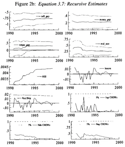
from (3.7) is not rejected either [F(6,63) --- 1.31 (0.315)]. Furthermore, no major problems are detected when the equation is used for producing one-step ahead forecasts over the last six years of the sample. When estimated recursively, the parameters in (3.7) turn out to be relatively constant over the recent period. Figure 2a records the time series of fitted and actual values of A ~ and the scaled residuals. Figure 2b shows a graphical summary of results from the recursive estimation of the equation over the 1990s.

Estimation results tend to give support to GS's claim that the real money gap has substantive predictive power for future inflation in the euro area, as evidenced by the significance of the term (rh-/h*)t_ 1 in

(3.7). Contrary to the predictions of the pure P-star model, (3.7) shows that the real money gap (or the price gap) is not a sufficient statistic for future inflation. This is consistent with the analysis in GS, who augment the basic P-star model with additional terms pertaining to a traditional Phillips curve model of inflation, giving rise to specification (3.1 a + 3. lb). Yet, the presence of additional terms in (3.7) indicates that the extended P-star model given by (3.1a + 3.1b) is badly mis-specified, though estimates do not provide any indication on whether the source of this mis-specification comes from (3.1) - i.e., the postulated extended P-star specification i t s e l f - or, most likely, from (3.2) - i.e., the postulated model for expectations formation. Investigating what structural model may give rise to the stylized facts encountered is far above the modest objectives set for this paper and will need to be addressed in future research.

3. W h a t L e a d i n g I n f o r m a t i o n i n t h e R e a l M o n e y G a p ?

In this section we further investigate the main conclusion in Section III.2 (namely that the real money gap has substantive predictive power

(18)

Figure 2a: Equation 3.7: Fit and Residuals

Dinf Fitted ~ 0 I i I I i i L I L i i I i i * . L I 1980 ! 985 1990 1995 2000 3 - Res dual

-,

?v/v

.2 I 1980 19S5 1990 1995 2000 39

for future inflation in the euro area) b y a n a l y z i n g the correlations at different t i m e h o r i z o n s b e t w e e n ( n - :t)t and the various indicators included in (3.7). Results in this r e s p e c t are reported in Table 3. M o r e precisely, the table shows e s t i m a t e s o f (3.8) b e l o w for f o r e c a s t i n g horizons ranging f r o m h = 1 to h = 8 quarters:

( ~ -

:t),+h_t = ~ (~,-1 - :t,) + ~ (r~- "~*),-1

+ a~3(Y-Y*)t-t + a~4 [(i~-1- ~ t ) - ( i s - r + ~t+h-I (3.8)

15

with Vt+h_ 1 following a M A ( h - 1) process.

15 It should be noted that for h=l, equation (3.8) is just a trivial re-parameterization of equation (3.7). Equation (3.8) is often interpreted as a forecasting equation. See, for instance, Stock and Watson (1999) and Clements and Hendry (1996).

(19)

Figure 2b: Equation 3.7: Recursive Estimates

- - i n f l g l l p .4 " - . . . . -.75 ~ .2 ~ - m o _ n c y ~ a p 1990 1995 2000 1990 1995 2000

:I

"I

9 f - - ~ J ~ " " ~ x - - r e a l r a t e j ~ .25 ~ . . . 1990 1995 2000 1990 1995 2000

00,,

'0I

. . .

00,,f J ~

'

.0,~

i i i i r i , i i , i L i I 1990 1995 2000 1990 1995 2000

;I ...

o,~ ~-,.,.., rx

~ o / ~

~-w- ~ v

~AAL"-'~'~"~

- . O l i - ? , I _ _ ~ , A , I 1990 1995 2000 1990 1995 2000

:I ...

. . . . - 5 % - - N d n C H O W s - 5 % - - N u p C H O W s 1990 1995 2000 1990 1995 2000

The results in Table 3 highlight the significant positive association that exists between the real money gap and future inflation. This significant correlation appears to extend over five to six quarters and reaches a maximum at the three-to-four quarter horizon. Consistent with the findings in Section 111.2, the real money gap does not come out of the analysis in the table as a sufficient statistic for future inflation. The two other gaps included in (3.7) - the output gap and the difference between the real short-term rate and the estimated equilibrium real short-term rate- also appear to contain valuable information over and above that already contained in the real money gap. According to the reported estimates, the correlation between the output gap and future inflation is indeed higher than in the case of the real money gap. It extends over six quarters and reaches a maximum at the five-quarter horizon. The lead-

(20)

Trecroci/Vega: The Information Content of M3 41 Ix# r~ - ! II o II II II II I= "r. II II II II II I I I I i ~ , ~1~ I I i ~ ~ ~ 'ml- o o o'~ I I I ** ,, T~ - ~ ~ O . . O o O < 2 ~ II ..= E = ._= "~ O . = _ + ~ ~ + - - tt~ o o ~ = i o

(21)

ing information contained in the real rates is short-lived, extending over just three quarters. Finally, results in the table also show how forecasting performance deteriorates dramatically as the time horizon increas- es, as evidenced by the sharp reduction in the R 2 of the regressions. None of the indicators analyzed appear to contain information that can be used to forecast inflation at horizons over 6 quarters.

Figure 3 illustrates further the main results above. It shows time series for inflation deviations from "target" together with the various gap indicators entering (3.8). The latter are lagged according to the evidence in Table 3 to allow for a better visual impression of the correlations found.

4. O n t h e R o b u s t n e s s o f t h e R e s u l t s

The empirical results so far obtained illustrate that leading indicator properties of M3 can be detected by augmenting the information set in CV to include potential output and a measure of the monetary authorities' (implicit) inflation objectives. In this extended framework, deviations from the "trend" of GDP inflation are explained as a function of the deviations of real money, real output and real short-term interest rates from their unobserved equilibrium values. All these variables involve measurement problems that we have somewhat obviat- ed by using some ad hoc empirical measures. This certainly introduc- es important caveats to the conclusions reached in the previous sec- tions and, moreover, makes it necessary to get a sense of how sensi- tive results are to changes in our empirical measure of the un-observables.

With a view to analyzing the robustness of the conclusions, estimates of (3.7) are reported in Table 4 for various empirical measures of ~t and y*. In the left panel of the table, R is estimated by OLS using the deterministic exponential trend postulated in GS, whilst a number of measures of potential output are alternatively employed, namely: the one contained in Fagan et al. (2001) 16 and several measures obtained by smoothing real GDP through the application of a standard Hodrick- Prescott (HP) filter with parameter A = 1600, 5000 and 15 000, respectively. In the right panel, the exercise is repeated for fixed y* (construct- ed using the HP filter with & = 1600) and for various HP-based measures of ~t.

16 Potential output is estimated therein from a Cobb-Douglas production function with smoothed Solow residuals.

(22)

0.04 0.03 0.02 0.01 O -0.01 -0.02 -0.03 -0.04 -0.05 1980 0,05

Figure 3:

Inflation Deviations from "Target" and Various Gap Indicators

0.05 0.04 0.03 0.02 0.01 0 -0.01 -0.02 -0.03 -0,04 -0.05

- - inflation (deviations from trend) ~ r e a l money gap (lagged 3 quarters)

--inflation (deviations from trend) - - o u t p u t gap (lagged 5 quarters)

1985 1990 1995

1980 0.05

4 3

--inflation (deviations from trend) ~ r e a l shod-term rates {deviations from equilibrium)

1985 1990 1995 0.04 0.03 0.02 0.01 0 -0,01 -0.02 -0.03 -0.04 -0.05

Trecroci/Vega: The Information Content of M3

(23)

44 W e l t w i r t s c h a f t l i c h e s A r c h i v 2002, Vol. 138 (1) r~ I-4 r t~ t ~ ~ t ~ q: o o " ~ ~ c 5 eq 9 II ~ c 5 c5c5 ~ 5 ~ c 5 r "~" r ~ c 5 c 5 ~ ~ ~ c 5 ~ c5 t'-- t'~ ~5 ~5 ~5 c5 c5 t ~ .o 0 a , - ~ e ~

(24)

Trecroci/Vega: The Information Content of M3 45 A number of conclusions can be drawn from the estimates in Ta- ble 4:

9 The real money gap enters significantly most of the specifications in the table, thereby confirming the leading indicator properties found above. Whilst estimates vary across specifications, this qualitative result appears to be robust to the different empirical measures of potential output employed. It seems also quite, but not totally, robust to the use of different empirical measures of the monetary authority's inflation objective.

9 The significance of the output gap in (3.6) appears to vary crucially with its own empirical measurement. The smoother the filter employed for deriving potential output, the less significant the output gap becomes in (3.6).

9 The reported estimates also show that the real interest rates and (to a lesser extent) the term spread also contain useful information for future inflation over and above that already contained in the real money gap and the output gap. This finding also appears quite robust across specifications.

IV. Encompassing Rival Models

In Section III.2, we estimated a model for GDP inflation which accounted for the most salient features of both GS and CV specifications. The estimated equation (3.7) was thoroughly evaluated against a number of statistical criteria. These included testing for homoskedastic innovation errors and constant parameters as well as testing for no information losses as we (following a general-to-specific approach) move along the reduction process to arrive at our preferred specification. That, in turn, ensures that the estimated model is data-congruent, in the sense that it matches the available evidence. Since "true" models may be expected to be congruent, congruency is an important operational criterion that may help discriminate between empirical models. How- ever, a model which is congruent is not necessarily 'true' 17 and a number of congruent models can be developed in empirical work. More- over, congruent models may not be nested, which complicates com- parisons between competing models.

~7 For instance, a stochastic process may be an innovation relative to a given information set but may be predictable when the information set is augmented, as already shown in Section Ili.2.

(25)

F o l l o w i n g M i z o n and R i c h a r d (1986) and H e n d r y and R i c h a r d (1989), we define a c o n g r u e n t e n c o m p a s s i n g m o d e l as a m o d e l which is c o n g r u e n t and which is able to a c c o u n t for, or explain, the results obtained by rival models. E n c o m p a s s i n g and f o r e c a s t e n c o m p a s s i n g - the criteria used t h r o u g h o u t this section for m o d e l evaluation - are m o r e stringent c o n c e p t s than ' b e t t e r fit' or (when applied in the context o f f o r e c a s t i n g ) ' l o w e r root m e a n square f o r e c a s t e r r o r ' , since it entails that no useful additional i n f o r m a t i o n is c o n t a i n e d in rival e v i d e n c e as well as v a r i a n c e / r o o t m e a n square f o r e c a s t errors d o m i n a n c e . 18

In the p r e s e n t context, one e x a m p l e o f a n o n - n e s t e d c o n g r u e n t m o d - el for G D P inflation can be f o u n d in F a g a n et al. (2001). In their m o d - el, G D P prices are d e t e r m i n e d in the long run by trend unit labor costs, which d e p e n d in turn on potential G D P and the N A I R U . In the short run, G D P inflation is e x p l a i n e d as a function o f c h a n g e s in trend unit labor costs, c h a n g e s in i m p o r t prices and deviations o f real trend unit labor costs f r o m equilibrium. E s t i m a t i o n o f the m o d e l o v e r the s a m p l e 1 9 8 0 : Q 4 - 1 9 9 7 : Q 4 p r o v i d e s the f o l l o w i n g results: A ~ t = 0.021 - 0.776 fft't_ 1 + 0.140 A w * + 0.068 A w * l (0.005) (0.109) (0.043) (0.047) + 0.136 Awt*_ 2 + 0.024 A p m t _ x - 0.274 ( p - w * - O)t_1 (0.045) (0.014) (0.076) T=69 (1980:Q4-1997:Q4) LM(1) = 0.22 (0.641) ARCH(4) = 0.48 (0.750) RESET = 1.55 (0.218) R 2 = 0.52 LM(4) = 0.23 (0.634) HET = 0.38 (0.964) FOR(24) = 16.019 (0.887) (4.1) o= 0.78% DW = 2.02 LM(1,4) = 0.54 (0.709) NORM = 4.12 (0.127) CHOW(24, 37) = 0.535 (0.945) w h e r e w* and p m stand for trend unit labor costs and i m p o r t prices, respectively.

With a v i e w to d i s c r i m i n a t i n g b e t w e e n the t w o c o n t e n d i n g m o d e l s , M i z o n and R i c h a r d ' s (1986) simplification e n c o m p a s s i n g tests (SET) w e r e conducted. Tests for (3.7) and (4.1), respectively, against the minimal nesting m o d e l p r o v i d e d the f o l l o w i n g results ( p - v a l u e s in brackets): F(7,58) = 1.518 (0.179) w h e n the null is (3.7) and F(4,58) = 0.599 (0.665) w h e n the null is (4.1). Therefore, b a s e d on w i t h i n - s a m p l e information, there a p p e a r s to be little to c h o o s e b e t w e e n both models19:

18 Ericsson (1992) reviews a number of measures of forecast performance, including encompassing, parameter constancy and mean square forecast errors. It shows that the two latter are necessary for 'good' forecast performance, but neither (nor both) is sufficient. See also Harvey et al. (1998).

19 Note also that the fits of the two models - as measured by their respective residual standard errors - are close.

(26)

none of the test statistics can reject at standard confidence levels that both models (3.7) and (4.1) are valid simplifications from the minimal nesting model. This inference appears to be stable when the test statistics are computed recursively over the sample 1992:Q1 - 1997:Q4.

We also tested for out-of-sample forecast encompassing, with forecasts under models (3.7) and (4.1) generated by using only lagged information. More precisely, the following equations were estimated recursively over the sample 1992:Q 1-1997:Q4 to produce 24 observa- tions of out-of-sample forecasts at horizons ranging from h = 1 to h = 8 quarters2~

(Ygt+h-1 -- "71~t-1) = ~1 ('7rt-1 -- ~7~t) + ~2 (?n -- g?~*)t-1

"1- ~3 ( Y - Y*)t-I 4" ~4 [ ( / t - I -

A t ) - ( is-

yl~')* ] "1-

~lt'~h-1

(4.2) 2

(a~t+h_l- .71~t_l) = /~h "t- ~h $1.t_ 1 +

i~=l[3himwt~i

2

-t- ~[~h i Apmt_ i

+ flh ( p - - w * -- 0 ) + ~2t+h-1. (4.3)

i=l

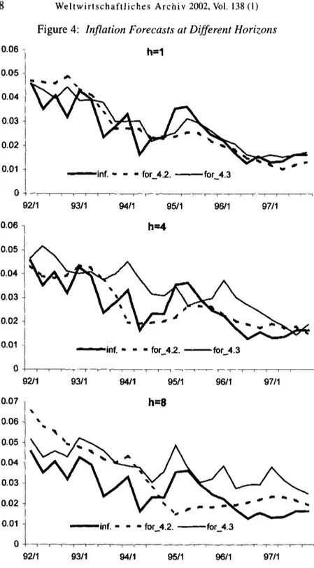
Figure 4 shows the resulting inflation forecasts at horizons of one (top panel), four (middle panel) and eight (bottom panel) quarters. Visual- ly, whilst (4.3) fares comparatively well at the one-quarter horizon, its performance deteriorates as the forecast horizon is extended. Converse- ly, (4.2) appears to outperform (4.3) at the four-quarter horizon, consistent with the finding above that the maximum correlation between the real money gap and future inflation is reached at that horizon. At the eight-quarter horizon, none of the models perform particularly well.

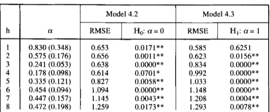
Table 5 reports the corresponding root mean square forecast errors at the one- to eight-quarter forecast horizons together with some tests for forecasting encompassing, zl When compared to the equation

2o In this exercise, the estimates of the different gap terms in (4.2) and (4.3) and, hence, the long-run parameters are based on end-of-sample information. Attempts to allow for recursive estimation of the long-run parameters fail to provide any systematic basis for comparison, giving rise to erratic results that proved to be difficult - if not im- possible - to interpret. This happens despite the lack of convincing statistical evidence about parameter non-constancy, which is rejected by formal tests. Accordingly, we interpret this finding as a reflection of the problems involved in conducting inference on cointegration and in estimating long-run relationships using small samples, rather than a problem of genuine parameter instability. It should be kept in mind, however, that the proposed exercise downplays the uncertainty surrounding inflation forecasts which could have been produced using only the information truly available in real time, as demonstrated in Orphanides and van Norden (2002) in relation to the measurement of the output gap.

(27)

0.06

Figure 4:

Inflation Forecasts at Different Horizons

h=l 0.0,5 0.04 0.03 0.02 0.01 inf. - = = for 4.2. ~ f o r _ 4 . 3 92/1 93/1 9411 95/1 96/1 97/1 0.06 _h=4 0.05 0.04 0.03 0.02 0.01 0

inf. - - = for_4.2, for_4.3

92/1 93/1 9411 95/1 96/1 97/1 0.07 0.06 0.05 0.04 0.03 0.02 0.01 0 h=8 I

inf. = = = for 4.2. for_4.3

(28)

Table 5: Root Mean Square Forecast Errors at the One- to-Eight-Quarter Forecast Horizons (h) and Tests

for Forecasting Encompassing

49 0.830 0.575 0.241 0.178 0.335 0.454 0.447 0.472 N o ~ : ** and Model 4.2 Model 4.3

a R M S E Ho: a = 0 RMSE HI: a = 1

(0.348) (0.176) (0.053) (0.098) (0.121) (0.094) (0.157) (0.198) * indicate significance at 5 0.653 0.0171"* 0.656 0.0011"* 0.638 0.0000"* 0.614 0.0701" 0.827 0.0058** 1.094 0.0000"* 1.145 0.0043** 1.259 0.0173"* 0.585 0.6251 0.623 0.0156"* 0.834 0.0000"* 0.992 0.0000"* 1.033 0.0000"* 1.148 0.0000"* 1.208 0.0004** 1.293 0.0078** and 10 percent confidence levels.

standard errors reported above, the results for h = 1 imply that both models fare particularly well during the period under analysis 1992: Q1 - 1997:Q4. In any event, Chow test statistics do not detect any structural break: Chow (24,41) = 0.508 (0.960) in the case of (3.7) and Chow (24,37) = 0.535 (0.945) in the case of (4.1). As regards forecasting encompassing, the table shows estimates of a (with standard errors consistent to autocorrelation and heteroscedasticity) as well as p-values for the null hypotheses H0: a = 0 and HI: ce = 1 in the regressions:

~ l t = 13~ (L~I t -- ~2t) "]" ~'t,

(4.4)

where ~ and ~ (h = 1 . . . 8) stand for the corresponding forecast errors obtained from (4.2) and (4.3), respectively. Rejection of one of the null hypotheses provides evidence in favor of the hypothesis that the rival model contains information which helps to explain forecast errors from the own model, i.e., (4.2) under H 0 or (4.3) under HI. This situation calls for forecast pooling, whereby better forecasts can be sought by combining the forecasts obtained from both models. As argued in Ericsson (1992), finding such a pooled forecast is primafacie evidence of both individual models being mis-specified.

The evidence in the table points to model (4.2) outperforming model (4.3) at the one- and two-quarter horizons. That reveals that the

(29)

P-star model may not be the best forecasting tool at short-term horizons. 22 Indeed, for h = 1 model (4.2) appears to incorporate little information which is not already contained in model (4.3). Conversely, the out-of-sample forecast record of the P-star model turns out to be comparatively better for all forecast horizons h > 3, though for h > 6 performance is rather poor for both models. More importantly, however, the encompassing hypotheses are rejected at all horizons other than h = 1. We interpret this outcome as an indication that, at those horizons, each model incorporates - though only partially - information which turns out to be relevant to explain inflation developments in the euro area.

V. Conclusions

The information content of M3 broad money for future inflation in the euro area was investigated from a number of perspectives throughout the paper. First, in Section II the leading indicator properties of broad money M3 were analyzed by conducting tests that money does not Granger-cause prices in the context of a cointegrated VAR system that has recently been proposed to investigate money demand in the euro area. The main finding is that there appears to be little empirical support for rejecting at standard confidence levels Granger non-causality of m on p within the information set employed therein. This conclusion is found to be stable throughout the sample and seems to be robust to re- ductions of the information set and to a number of plausible assumptions concerning: (i) the maximal degree of integration of the variables in the system;

(ii)

the lag length selected for the VAR; and

(iii)

the im- position or not of the long-run homogeneity o f m andp, though the long- run homogeneity hypothesis cannot be rejected at standard confidence levels.

We further investigated in Section III the leading indicator properties of broad money M3 by looking at the recent claim that - in the context of a P-star model - the real money gap (i.e., the gap between current real balances and long-run equilibrium real balances) has substantial predictive power for future inflation in the euro area. We show that

22 Indeed, it could be argued that both models are of little practical use at very short horizons, since there exist alternative non-causal statistical devices which typically fare pretty well at those horizons. For instance, if the interest is forecasting GDP inflation in a given quarter, one is likely to do better by using within-the-quarter monthly information in HICP or other price indices which are available ahead of the publication of GDP inflation.

(30)

this empirical finding can be reproduced when the information set employed in Section II is augmented to include variables such as potential output and the monetary authorities' implicit inflation objective. Whilst these variables are not directly observable and, therefore, problems may certainly exist when it comes to measuring, we believe that they must enter any empirical model of inflation which is claimed to be theory- consistent. The results in this section illustrate the claim made in the Introduction that inference about Granger non-causality may vary with the information set at hand and confirm that a significant positive association exists between the real money gap and future inflation up to five-to-six quarters ahead, reaching a maximum at the three-to-four quarter horizon. This stylized fact appears to be quite, though not totally, robust to the use of a number of empirical measures for the two un- observables.

When it comes to providing structural interpretations of these findings, the results are, however, less satisfactory for the P-star model of inflation. We showed, also in Section III, that the real interest rate and (to a lesser extent) the term spread appear to contain information that can be used to forecast inflation developments which are left unex- plained by the P-star model of inflation. This in turn suggests that the treatment of inflation expectations and most possibly the measurement of the monetary policy authorities' implicit inflation objective needs at least to be refined.

Finally, in Section IV we compared the model developed in the previous section with an alternative model for GDP inflation in the euro area with no explicit role assigned to money. In the latter, prices are de- termined in the long run by trend unit labor costs, which depends in turn on potential GDP and the NAIRU. In the short run, GDP inflation is explained as a function of changes in trend unit labor costs, changes in import prices and deviations of real trend unit labor costs from equilibrium. The comparison between the two models was made on the basis of their relative performance in explaining inflation developments in the euro area, both within and out of sample. The evidence in this section points to the P-star model outperforming the rival model at forecast horizons h > 3 and being outperformed by the alternative model at shorter horizons. The encompassing hypothesis (i.e., the hypothesis that no useful information is contained in the rival model) is, however, rejected at all horizons other than h = 1. On the basis of this evidence, we conclude that each model appears to have strengths of its own: both of them incorporate some information which turns out to be relevant to explaining GDP inflation; both of them, however, also fail to provide on

The information content of M3 for future inflation in the euro area