3D position estimation using deep learning

(1)

POLITECNICO DI MILANO

School of Industrial and Information Engineering Department of Electronics, Information and Bioengineering Master of Science Degree in Computer Science and Engineering

3D Position Estimation Using Deep Learning

Internal Supervisor: Prof. Giacomo Boracchi Politecnico di Milano

External Supervisor: Prof. Magnus Boman Royal Institute of Technology

Master Thesis’s by: Filippo Pedrazzini, 879110

(2)

(3)

(4)

(5)

Abstract

The estimation of the 3D position of an object is one of the most critical topics in the computer vision field. Where the final aim is to create automated solutions that can localize and detect objects from images, new high-performing models and algorithms are needed. Due to lack of relevant information in the single 2D images, approximating the 3D position of an object can be considered a complex problem. The single specific task of estimating the 3D position of a soccer ball has been investigated. This thesis describes a method based on two deep learning models: the ball net and the temporal net that can tackle this task. The former is a deep convolutional neural network with the intention to extract meaningful features from the images, while the latter exploits the temporal information to reach a more robust prediction. This solution reaches a better Mean Absolute Error compared to already existing computer vision methods on different conditions and configurations. A new data-driven pipeline has been created to deal with videos and extract the 3D information of an object.

Keywords: Convolutional Neural Network, Deep Learning, Computer Vision, 3D Object

Localization.

(6)

(7)

Sommario

La stima della posizione 3D di un oggetto può essere considerata uno degli aspetti più importanti nell’ambito intelligenza artificiale. Dove l’obiettivo finale è quello di creare soluzioni automatizzate in grado di localizzare e rilevare oggetti dalle immagini, è neces-sario lo sviluppo di nuovi modelli e algoritmi ad alte prestazioni. A causa della mancanza di informazioni rilevanti nelle singole immagini 2D, l’approssimazione della posizione 3D di un oggetto può essere considerato un problema complesso. Il singolo studio relativa-mente alla stima della posizione 3D di una palla da calcio è stata investigata in modo specifico. Questa tesi descrive un metodo basato su due modelli neurali: ball net e

temporal net. La prima è una rete neurale convoluzionale con l’intenzione di estrarre

caratteristiche significative dalle immagini, mentre la seconda sfrutta le informazioni temporali per ottenere una stima più accurata. Questa soluzione raggiunge un errore assoluto medio migliore rispetto ai metodi di computer vision esistenti in condizioni e configurazioni diverse. Una nuova data-driven pipeline è stata creata per gestire video ed estrarre le informazioni 3D di un oggetto.

(8)

(9)

Acknowledgments

I would like to thank professor Boracchi for giving me support during the thesis. I would also like to thank the people at KTH who supported me, most notably my supervisor Magnus Boman and my examiner Henrik Boström.

Moreover, I would like to thank Matteo Presutto for giving me access to his GPU server, making the training of the models possible.

Finally, I want to express my profound gratitude to my family who helped and sup-ported me during these years in every occasion and each decision I took. Thank you for the love that you gave me.

Milan, July 12, 2018

Filippo Pedrazzini

(10)

(11)

List of Figures

1.1 The final pipeline used for the prediction. . . 5

2.1 The pin-hole camera model. . . 9

2.2 The pin-hole camera model with the intrinsic uncertainty in the recon-struction of a 3D point. . . 10

2.3 The Artificial Intelligence (AI) landscape in terms of algorithms fields. . . 12

2.4 The Perceptron architecture. . . 13

2.5 Example of Feed Forward Neural Network with a single hidden layer. . . . 14

2.6 On the left the Sigmoid Activation function and on the right the respective derivative. . . 16

2.7 On the right Rectified Linear Unit (ReLU) activation function and on the left its derivative. . . 17

2.8 The Leaky ReLU activation function and its derivative. . . 17

2.9 Starting from left an example of underfitting, well fitting and overfitting curves. . . 20

2.10 Example of Dropout during training. . . 22

2.11 Example of Convolutional Operation. . . 23

2.12 Example of filter used to detect edges in images. . . 23

2.13 Example of Max Pooling Operation. . . 24

2.14 From left (low) to right (high) an example of features extracted using a Convolutional Neural Networks. . . 24

2.15 The ResNet architecture. . . 25

2.16 Example 1D convolutions; where D is the embedding dimension, W the filter width, and F the number of filters. . . 26

2.17 Example of RNN unrolled. . . 27

2.18 Example of Long Short-Term Memory (LSTM) cell. . . 28

2.19 Example of sample in the ImageNet Dataset . . . 35

2.20 Example of images in the NYU Depth Dataset . . . 37

3.1 Example of an image extracted using Unity engine. . . 41

3.2 Example of a a random trajectory generated using Unity. . . 42 X

(15)

3.3 An illustration of the data generation step . . . 43

3.4 The coordinates system origin . . . 44

3.5 The new origin of the coordinates system . . . 44

3.6 The co-planar points extracted with Unity for the Camera Calibration procedure. . . 46

3.7 The no-coplanar points extracted with Unity for the Camera Calibration procedure. . . 47

3.8 The first recurrent architecture used for training. . . 47

3.9 An example of extracted size feature. . . 49

3.10 The new recurrent architecture used for training. . . 50

3.11 The 1D Convolution architecture. . . 51

3.12 The 1D Convolution architecture for the classification task. . . 53

3.13 Example of input image (814, 1360). . . 58

3.14 Example of filtered image after the first convolutional layer (406, 679). . . 58

3.15 The deisgn network to estimate the (x, y, size) features. . . 59

3.16 The combination of the explained models in a unique single pipeline. . . . 61

4.1 Example of prediction on a test sample. . . 68

4.2 The Neural Network implemented for comparison purposes. . . 69

(16)

List of Tables

3.1 The first structured dataset columns used for training. . . 42 3.2 The new structured dataset columns. . . 49 4.1 The baseline scores using different configurations and number of frames. . 65 4.2 The scores of the first deep approach compared to the baseline method. . 65 4.3 The new deep approaches compared to the baseline . . . 66 4.4 The results of the binary classification task in terms of accuracy. . . 67 4.5 The results of the more general task of estimating the 3D position of the

ball. . . 67 4.6 The final results over the real values and the predictions of the ball net. . 68

(17)

Acronyms

AI Artificial Intelligence.

ANN Artificial Neural Network. BCE Binary Cross Entropy. FPS Frames Per Second.

LSTM Long Short-Term Memory. MAE Mean Absolute Error. MSE Mean Squared Error. ReLU Rectified Linear Unit. RMSE Root Mean Squared Error. RNN Recurrent Neural Network.

(18)

(19)

Chapter 1

Introduction

This chapter has the objective to give an introduction to the problem and purpose of the work, ending up with the description of how the thesis is structured.

1.1 Background

Since the beginning, the objective of computer vision was to build a machine able to simulate the human ability of understanding, processing and extracting high-level fea-tures from images and videos, with the final aim to create automated solutions that could imitate human tasks with a high level of accuracy. The goal is to make computers able to recognize, detect and classify objects without any human assistant. The field has been investigated for a long time due to the exciting aspects of automation and the multiple use cases in which it can be exercised. After years of development in the same direction, where the application of geometric-based solutions has been manipulated, a revolution in the field happened in 2013 [1]; the first deep learning approach came out to solve an object detection task without any assumption on the environment. From that moment on, deep learning has been used to address more and more difficult tasks, creating a worldwide competition for the fastest and most accurate algorithm.

When dealing with soccer statistics a manual solution is still used to gather real-time highlights. The aim for an automatic solution is to reconstruct real-time statistics from soccer videos matches without involving the human labor. At the moment, the mar-ket has different products to achieve a data-driven analysis of games and performances. More specifically, the primary objective of these solutions is to accurately detect each player and the ball in the field to compute some essential highlights about the match. In the case of soccer, highlights are highly correlated with the 3D position of each object in the field. With the ball and players information, a simple analytical method

(20)

2 1.2. PROBLEM

can be used to have aggregated data useful for additional improvements and analysis. A data-driven approach can be used to detect the object position in the image. The first strategies came out years ago following a geometrical computer vision solution: [2], [3], [4], [5], [6], [7] and [8]. All of them shares the same paradigm used to find a final solution:

1. Computing the projection matrix. 2. Detecting the object within the image. 3. Estimating the 3D position of the object.

On the other hand, the deep learning growth led to more performing models that can tackle, and that can be engaged to find more robust and accurate results. The estimation of the object’s position relative to the court system of coordinates requires advanced and robust techniques. This work introduces a solution to accurately predict the 3D position of an object using the union of deep learning strategies.

1.2 Problem

In just a few years, a massive revolution in the computer vision industry took place, mov-ing the research toward the deep learnmov-ing field. Considermov-ing these significant advance-ments, estimating the object coordinates in an image can be seen as a solved problem, but when the goal is to reconstruct the 3D position from a video coming from a single camera, still much work is needed to achieve a good result. From the 2D information, we can reassemble the 3D position of an object under specific requirements; if all the objects lay on the same plane, a comprehensive mapping can be created using the camera matrix; a deep explanation regarding the geometrical problem will take place in the next chapter. In the soccer domain, the players preserve one coordinate equal to zero, which is the requirement needed to reconstruct their position in the court coordinates system. For this reason, the 2D location within the images that can be extracted using state of the art deep learning techniques are enough to build a model able to deliver statistics about the teams. While the players tracking can be easily solved, the estimation of the ball 3D position can be recognized as a more complicated issue. The object size and the physic behaviour make the task more challenging to face, both concerning detection and reconstruction. The presence of the third coordinate makes the 3D prediction more complicated, and the solution cannot just be based on the previously mentioned camera matrix. Camera matrix, projection matrix and camera calibration, they all refer to the same process of computing the model that maps the 3D coordinates system to the cam-era one (2D). In the following chapter, a detailed intuition about the concepts will take place.

(21)

CHAPTER 1. INTRODUCTION 3

[2] and [5] tried to solve the same problem using domain-specific information regarding the soccer field and the physical constraints of the ball. On the other hand, deep learning state of the art techniques were not available ten years ago, and the need to create a more recent and advanced procedure employing new artificial intelligence methods is required. Following the discussion; this work addresses the problem of estimating the 3D loca-tion of an object starting from 2D videos; more specifically, having a sequence of images from a single fixed camera, a data-driven algorithm should predict the 3D position of an object relative to the environment system of coordinates. Given these assumptions, the implicit research question regards the success of the solution.

“Having a single fixed camera is it possible to extract the 3D position of an object accu-rately using a data-driven approach?”

1.3 Goal

The goal of this work is to investigate and create a method that can solve the problem of estimating the 3D coordinates of a soccer ball without any assumption of the court characteristics starting from a video. The combination of deep learning techniques could lead to a significant result concerning accuracy. Due to the lack of meaningful existing solutions, some metric criteria have been created to evaluate the work. A robust solu-tion would mean to create a product or an architecture that can be adapted to other applications. Some steps are required to achieve this result:

1. Collecting data: creating a comprehensive dataset to train and test the designed models.

2. Define a model to solve the task: iterating over the assumptions and configurations a deep learning model should be designed to predict the labels accurately.

3. Tune the parameters: adjusting the hyper-parameters for better performances. 4. Analyzing the results: reflecting over the obtained scores to possible further

im-provements.

1.3.1 Benefits, Ethics and Sustainability

The introduction of a method able to capture the 3D position of an object having as input a sequence of images can be useful for many different applications. Where the requirement is to localize an object in the 3D space having a single camera, the em-ployment of the same paradigm can be lead to a performing estimator. On the other

(22)

4 1.4. METHODOLOGY

hand, when dealing with the specific case of soccer, the introduction of highly accurate performing computer-based solutions can substitute the currently manual work of gath-ering statistics. The need for maintenance and performance assurance is still required, but different expertise is needed to face the task of managing a smart machine.

From a sustainability perspective, many are the domains in which the estimation of the 3D position of an object can bring added value and help improving people life. An example is the Augmented Reality industry where most of the applications address the problem of helping sick people in the daily life creating products that can help them to track and localize objects in the environment. Another example is the autonomous driving cars industry; the core technology has been changed from sensor-based solutions to computer vision methods. The possibility to precisely track people and obstacles is required to have a safe machine.

1.4 Methodology

An empirical approach has been followed to achieve a robust result. Due to the limited number of related works, different implementations have been tested before ending up with a meaningful answer. A quantitative analysis was mandatory to find the most suit-able model. A quantitative data collection was required to train and test the models. On the other hand, the quality of the performances is strictly related to the domain field in which the solution is applied. For this reason, a qualitative analysis associated with the effectiveness of the answer has been discussed toward the obtained results. A single case study has been investigated to validate the effectiveness of the architec-ture, which can not be considered enough to generalize the solution to different domains. The complexity of the problem led to the first decision of splitting the issue into different and simpler tasks:

1. 3D trajectory extraction: the reconstruction of the 3D position of the ball while doing a trajectory (flying).

2. Flying - not flying classification: the binary classification regarding the flying:not-flying position of the ball.

3. Object detection and Size estimation: the detection of the 2D coordinates of the ball as well as the estimation of the size of the object in the 2D images.

The result is the union of two deep learning models ball net and temporal net; the former is a convolutional neural network that has the objective to extract the images informa-tion; while the latter is a shallow network with the intent of extracting the temporal

(23)

CHAPTER 1. INTRODUCTION 5

information for a better prediction. In Figure 1.1 an illustration of the final model. A final Mean Absolute Error (MAE) of 1.3 has been reached using the combination of these two networks in the prediction of the (x, y, z) position of the ball in the soccer environment.

(24)

6 1.5. DELIMITATIONS

Due to lack of data, a synthetic dataset using Unity [9] has been created to simulate a real-case scenario and to test the methods over a meaningful simulation, providing scores relative to the given environment.

This work illustrates the followed path to achieve a performing model. Each step rep-resents a move toward the direction of finding a suitable and robust solution for the problem mentioned above. The design choices are explained progressively in order to deliver to the reader a logical flow of decisions and improvements.

1.5 Delimitations

The main limitation regards the data employed when dealing with this specific task; a synthetic dataset has been used to validate the architecture, but in case of a real dataset the same performances could not have been reached. A secondary limitation regards the generalization of the solution. The work addresses the problem of finding a data-driven approach that could be employed in different domains, but here a single case study has been investigated. Where specific configurations and characteristics regarding the data are not satisfied, the same performances could not be obtained compared to the investigated task.

1.6 Outline

The second chapter gives a detailed intuition of the related works of the field and how the thesis can benefit from the investigation of these methods. The basic concepts are explained to give the reader the possibility to understand all the thesis technologies and phases. Moving on, the third chapter includes the explanation of the empirical method followed to create a robust implementation to solve the explained research question effec-tively. Next, the fourth chapter presents the results obtained using the models designed and explained in chapter three. The fifth chapter illustrates the possible applications and problems of the implemented product. Finally, the sixth chapter concludes answering the research question and possible further improvements.

(25)

Chapter 2

Theoretic Background

The chapter contains the literature study performed to have insight regarding the state of art approaches in the computer vision field and the related papers that tried to address the same research problem. The basic concepts regarding machine learning are explained in order to let the reader understand all the thesis phases.

2.1 Geometrical Concepts

2.2 Prerequisites

2.2.1 Homography

A homography is a 2D projective transformation from one system of coordinates to another. A homography H maps 2D points in homogeneus coordinates according to:

   x0 y0 z0   =    h1 h2 h3 h4 h5 h6 h7 h8 h9       x y z    (2.1)

Homogeneus Coordinates are a useful representation; if we normalize having w = 1

we obtain the unique image coordinates (x, y). For this reason, the homography H (3 × 3

matrix has eight independent degrees of freedom. 2.2.2 The Direct Linear Transformation

Homographies can be computed using the points of two system of coordinates. As

mentioned above a homography has eight degrees of freedom. Each point correspondence

(26)

8 2.2. PREREQUISITES

gives two equations, one each for the x and y coordinates, and for this reason four points are required to compute H.

The direct linear transformation (DLT) is an algorithm for computing H given four

or more mappings. Solving the equation Ah = 0 where A is the matrix containing two rows for each mapping, H can be computed.

         −x1 −y1 −1 0 0 0 x1x01 y1x01 x01 0 0 0 −x₁ −y₁ −1 x₁y0₁ y1y10 y01 −x2 −y2 −1 0 0 0 x2x02 y2x02 x02 0 0 0 −x2 −y2 −1 x2y02 y2y20 y02 ... ... ... ...                            h1 h2 h3 h4 h5 h6 h7 h8 h9                   = 0 (2.2)

2.2.3 The Camera Matrix

The camera matrix can be decomposed as:

P = K[R|T ] (2.3)

• R (3 × 3) in 2.3: is a rotation matrix that describes the orientation of the camera. • T (3 × 1) in 2.3: is 3D translation vector that explains the position of the camera

center.

• K (3 × 3) in 2.3: is the intrinsic calibration matrix that describes the projection properties of the camera.

The intrinsic matrix depends only on the camera properties and is in a general form written as: K =    af 0 cx 0 f cy 0 0 1    (2.4)

• f: is focal length which corresponds to the distance between the image plane and the camera center.

(27)

CHAPTER 2. THEORETIC BACKGROUND 9

With this assumption, the matrix becomes:

K =    f 0 cx 0 f cy 0 0 1    (2.5)

The remaining points are c = [cx, cy] which correspond to the coordinates of the

optical centre, the image point where the optical axis intersects the image plane. These values are often assumed as half the width and height of the image.

2.2.4 From 3D to 2D - The Pin-Hole Camera Model

The pin-hole camera model is the relationship between a point in the 3D space and its projection in the image plane. In Figure 2.1 an illustration.

Figure 2.1. The pin-hole camera model.

The relationship can be expressed as:

ax= P X (2.6)

Where the 3 × 4 matrix P is the camera matrix explained above. Having the in-formation about the projection matrix, that can be easily computed using the Direct Linear Transformation and some known points (3D and 2D), we can transform each 3D point into the 2D representation from the camera perspective.

2.2.5 From 2D to 3D

While a linear mapping can be identified between the 3D to the 2D representation, the problem of transforming a point from the 2D coordinates of the image plane to the 3D

(28)

10 2.2. PREREQUISITES

system of coordinates cannot be easily solved. If we assume the points in the 3D system of coordinates written in terms of homogeneous coordinates (X, Y, Z, K)T _{and let the}

centre of projection be the origin (0, 0, 0, 1)T _{with the image points represented in terms}

of homogeneous coordinates (x, y, z)T_{; the mapping can be represented, as previously}

explained, by a 3 × 4 projection matrix P with the linear system:

   u v w   = P3x4       x y z k       (2.7)

From the 2D information, the 3D reconstruction cannot be performed accurately since each point on the projection plane could lie anywhere on a ray from the camera through the plane. In Figure 2.2 an illustration of the problem from a visual perspective.

Figure 2.2. The pin-hole camera model with the intrinsic uncertainty in the

reconstruction of a 3D point.

Two possible solutions are available to solve the problem:

1. Same Laying Plane: if all the objects belong to the same z plane, the projection matrix can be computed using some of those points constraining the problem to a 2D to 2D mapping in the homogeneus coordinates. Assuming, for example, z = 0; the projection matrix can be computed using the Direct Linear Transformation and the linear mapping will be reduced to:

   u v w   = P3x3    x y t    (2.8)

(29)

2. Distance Between Object and Camera: referring to Figure 2.2, the missing infor-mation necessary to correctly reconstruct the position (x, y, z) given (u, v) is the distance between the 3D point and the camera center 0. If for each 2D point we can gather the value w, which represents the missing information, a complete mapping can be computed without taking care of the fact that all the 3D points should lay on the same plane.

2.3 Deep Learning Prerequisites

The objective of this section is to give an insight into the most meaningful concepts that have been employed during the thesis and that actively contributed to the design of a practical solution.

2.3.1 Introduction

AI has been part of the world history for a long time. Starting from the Turing test [10], the willing to create a smart machine increased over the years. Turing predicted that the first intelligent machine able to beat his experiment would have been invented with the opening of the new century (2000). In 2018, still, a performing solution to solve the test has not been developed. Recently, a new prediction by AI worldwide experts resulted in the delay of almost 30 years compared to Turing opinion. On the other hand, the need for a general purpose machine is not always required. For this reason, the first impressive returns in the AI field came out in the last few years, resulting in an incredible extension regarding investments. The exponential growth concerning the computational power and the generated data made these first solutions available. When dealing with AI, several different fields of expertise are present; each one of them has the objective to simulate the specific human behaviour and reach a certain level of accuracy or abstraction. Here an intuition for each macro-category:

1. Reinforcement Learning: agents capable to self-learn the patterns of a specific environment. They are mostly employed to solve optimization problems when an environment is defined, and certain predefined actions can be performed. Recent advancement brought to the combination of this field to the one of deep learning to deal with complex environments creating a new field known as Deep Reinforcement Learning.

2. Deep Learning: represents the branch of AI that deals with unstructured data (e.g., audio, images, speech, text). The growing computational power gave the oppor-tunity to develop deep models able to better perform and generalize over different complex tasks. The ANN invention was the first move toward the investigation of these new set of models.

(30)

12 2.3. DEEP LEARNING PREREQUISITES

3. Machine Learning: all the algorithms able to learn a pattern in the data minimizing a defined loss function.

In Figure 2.3 the AI landscape and how the different fields are connected and related to each other.

Figure 2.3. The AI landscape in terms of algorithms fields.

The next subsections will take care of explaining the basic deep learning concepts and the algorithms that the work exploited to obtain a final performing pipeline.

2.3.2 ANN

The Perceptron ANN is an AI model able to learn patterns in the data trying to

emulate the human brain. In fact, the human brain is composed of many neurons in-terconnected between each other that process the information and send the transformed signal to the next neuron. The first statistical model has been designed by Rosenblatt with the introduction of the Perceptron [11] in 1957. Even if the model is composed of a single neuron, it represents the basic concept behind the modern neural networks. The objective of this neuron is to learn the mapping between a specific input and a particular output (target). In Figure 2.4 the Perceptron structure is shown, where x[i] represents the input features and y the predicted output.

Each input features x1, x2, x3, . . . xnis multiplied with a single weight wiand the obtained

values are then summed with a bias term (1) to be fed into the single neuron. The sum is then processed using an activation function resulting into the output y equals to +1 if w0+ w1x1+ · · · + wnxn>0, and −1 otherwise, described as g(PNi xiwi). The weights

(31)

Figure 2.4. The Perceptron architecture.

(w0, w1. . . wn) are randomly initialized and learned during the training procedure using

the Hebbian rule [12]; at each observation, the error is computed between the model prediction and the actual value and then the weights updated accordingly to the rule:

wi← wi+ δwi (2.9)

E= ˜y − y (2.10)

δwi = αExi (2.11)

The data pattern is detected minimizing the error function updating the corresponding weights after observing each sample. ˜y represents the actual value and y the Perceptron prediction computed as y = g(PN

i xiwi). α describes the learning rate value, which is

the dimension of the update step. If the problem is linearly separable, the architecture is guaranteed to converge after a certain number of epochs. When dealing with more complex problems where the decision boundary is not a straight line, the need to add more layers and neurons is required. For this reason, the concept of feed forward neural network has been introduced.

Feed Forward Neural Networks A Feed-Forward Neural Network is an ANN which

employs several hidden layers composed of a certain number of neurons. The model learning capabilities are increased due to the presence of a certain amount of neurons each one of them employing non-linear activation functions (h() in Figure 2.5); each layer can be seen as a features transformation step that helps in the identification of

(32)

information able to reduce the defined loss function. In Figure 2.5 an example of Feed Forward Neural Network with a single hidden layer is provided.

Figure 2.5. Example of Feed Forward Neural Network with a single hidden layer.

As in the Perceptron, the task of finding the weights that best solve the problem of finding a pattern between the input and the output is defined. The difference is represented by the used technique to update the weights. As a matter of fact, backpropagation is used to achieve this scope and propagate the error over the different layers to update the weights employing a similar rule as the one of the Perceptron. The update rule is defined as:

wi← wi− α

∂E(θ)

∂wi (2.12)

At each observation, the error is computed, and the derivative obtained with respect to the weights propagated through all the layers of the network. The received value is then subtracted to the current weight wi performing a step in the direction where

the loss function is minimized. Since the weights are updated accordingly to the error derivative, a requirement regarding the activation function regards the differentiability; the non-linear activation functions are chosen taking care of this need.

2.3.3 Error Functions

Based on the problem that the ANN has to solve a different loss function is required. The majority of the tasks can be divided into two substantial categories: regression and classification. The former represents the work of predicting a continuous target value given a specific input features, while the latter represents the estimation of the

(33)

discrete value which the input should belong to. Based on the problem a different loss function is used to deal with the defined task. In case of regression Mean Squared Error (MSE) is used to represents the distance between the prediction and the actual value; while for classification cross entropy is the most suitable to represents the probability to belong to a particular class. Both have been derived considering an assumption on the distribution of the data. In case of regression, the target is normally distributed, while for classification purposes a multinomial distribution represents the distribution of the different classes C. M SE = 1 n n X i=1 (yi− xi)2 (2.13) Eentropy = − n X i=1 X y_k=1C y_i0klog (yk_i) (2.14) 2.3.4 ANN Hyperparameters

Hyperparameters are all the parameters that are not learned intrinsically during the training of the model while minimizing the defined loss function. The decision over these kinds of settings is of crucial importance in the deep learning field, on the other hand, they represent the most challenging task in the design/training of a deep learning model; the number of possible combinations and the need to train over a considerable amount of data makes the problem tough to tackle when hardware requirements are not met. Many methods have been investigated to find those values in a faster way taking care of saving concerning hardware performances. When the employment of a deep neural network is required, some design choices are necessaries to create a model able to solve the defined task. Different parameters are present concerning the architecture structure. The decision over activation functions, weights initialization methods, optimizers is a crucial point when developing the network structure. New techniques have been invented to facilitate the training convergence of the model. Indeed, the convergence of a neural network represents the most challenging task in the training procedure of a deep learning model. Often, due to the complexity of the error surface and the presence of many local optima, the difficulty of reaching the optimal solution is present. New optimizers, weights initialization methods and activation functions have been designed to overcome this problem. Following, a brief description of the most effective ways.

2.3.5 Activation Functions

Sigmoid and Tanh represents the most known activation functions; which have been employed for a long time due to non-linearity characteristics and the easiness in the

(34)

differentiability. At the same time, they cannot be engaged when many layers are in-volved in the network design. Taking Sigmoid as the example, the function is displayed in Figure 2.6 with its derivative.

S(x) = 1

1 + ε−x (2.15)

Figure 2.6. On the left the Sigmoid Activation function and on the right the

respective derivative.

As above mentioned, the weights are updated using back propagation, which means that each layer propagates the error to the previous layer accordingly to the derivative computed with respect to a specific weight. On the other hand, the maximum value of Sigmoid derivative (in Figure 2.6) is obtained when the input is 0 and is represented by a low number (0.25).

Multiplying a low number recursively at each backward step will result in a gradient amount close to zero in the first hidden layers of the network. This behaviour is called

gradient vanishing. The same pattern can be seen when employing Tanh as activation

function; even if the maximum gradient value is 1, most of the times the input will lay in a range of values that are not close to zero. A new activation function has been designed to solve the task: ReLU.

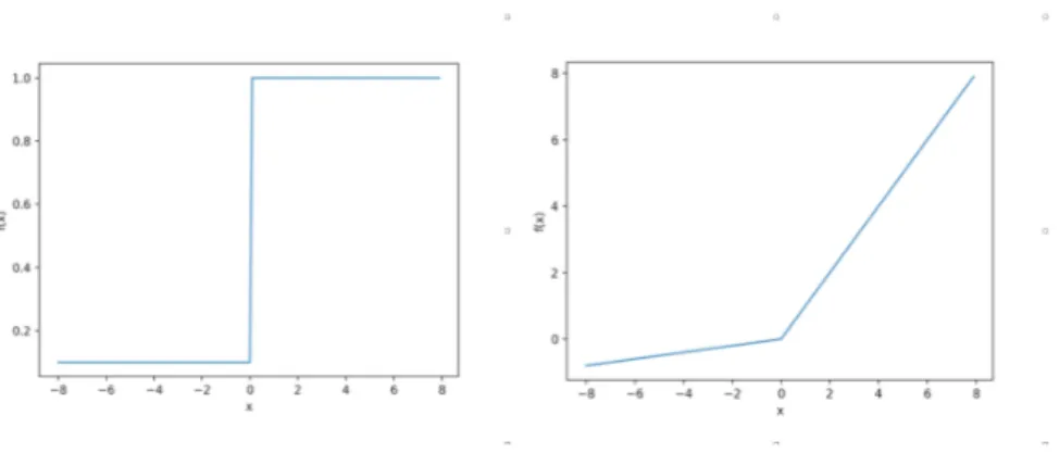
ReLU described as y = max(x, 0), does not suffer from the gradient vanishing issue since the derivative, if the input is greater than zero, is always 1. The gradient can be propagated over the different layers without taking care of the problem of low values in the first hidden layers. In Figure 2.7 ReLU activation function and its derivative.

On the other hand, ReLU suffers from another problem known as dying ReLU which is encountered when the activation function outputs a value that is always zero. Due to the flat characteristic of the activation function, when the input is lower than zero, the activated output will always be zero leading to the death of the neuron. At the moment that a neuron is dead a difficulty in the recovering phase is present since the gradient will

(35)

Figure 2.7. On the right ReLU activation function and on the left its derivative.

always be zero and the optimizer will not alter the weights correlated to that neuron. To solve the problem a bias term initialization should be used or another similar activation function employed; Leaky ReLU described as y = max(x, 0.001) is applied to solve the task. The only difference regards the behaviour of the function for values lower than zero. A small amount (0.001) is multiplied by the input to avoid to stack into a constant zero value causing the death of the neuron. In Figure 2.8 the activation function and its derivative are displayed.

Figure 2.8. The Leaky ReLU activation function and its derivative.

Other activation functions have been designed to improve the convergence of deep learning models (Elu [13], PReLU [14], Swish [15]), but a similar pattern has been exploited compared to ReLU.

2.3.6 Weights Initialization

Weights initialization represents the method used to initialize the weights when the algorithm has not started yet to learn the pattern from the provided data. The starting point is of crucial importance to converge faster and better. Many ways are present to

(36)

deal with this scope. Both simple and more complicated techniques are available; here a brief introduction of the possible most known methods is given.

All zero initialization Initializing all the weights to zero can be considered a mistake

because during backpropagation all the weights will compute the same gradients resulting in the same updates while different weights should learn different patterns to minimize the loss function.

Small Random Numbers A simple solution is to initialize the weights with a random

value close to zero with a Gaussian distribution. Even if the method can be useful in a lot of problems, it does not take into account a crucial aspect: uncalibrated variance. The variance of the randomly initialized weights output grows with the number of inputs (features). Considering z =PN

i xiwi with weights w and inputs x the variance of z is:

V ar(z) = V ar( N X i xiwi) (2.16) = N X i V ar(xiwi) (2.17) = N X i

[E(wi)]2V ar(xi) + E[(xi)]2V ar(wi)+ = V ar(xi)V ar(wi) (2.18)

= N X i V ar(xi)V ar(wi) (2.19) = (nV ar(w))V ar(x) (2.20)

Calibrating the Variance To solve the problem mentioned above, we can normalize

the assigned value with the number of inputs (fan-in) as following (where N represents the standard normal distribution):

W ∼ N√1

n (2.21)

If the objective is to have the variance of z equals to the variance of all its inputs

x, the initizalization of each weights w should be 1/n. With this simple technique

better convergence can be obtained because all the neurons in the network initially have approximately the same output distribution.

Xavier Initializer Glorot and Bengio in [16] proposed a new initialization method

(37)

in the next layer (nj+1), empirically proving a better convergence over complex tasks.

V ar(W ) = 2

nj+ nj+1 (2.22)

2.3.7 Optimizers

The optimizer represents the rule that we use to update the network weights with respect to the obtained derivative. Many different optimizers are present, and a brief intuition for the most famous ones will be lead in the current Subsection.

Gradient Descent Gradient Descent represents the most used optimizer when dealing

with deep learning models; the adopted rule is defined in Paragraph 2.3.2 where the explanation of back propagation has been taken. Three different variants of Gradient Descent are available; the main difference regards the amount of data used to compute a single weights update.

1. Batch Gradient Descent: the entire train set is used to compute the gradient and update the weights.

2. Stochastic Gradient Descent: a single example is employed to compute the gradi-ent.

3. Mini-Batch Gradient Descent: a set of samples is considered to update the weights. In terms of convergence, a difference is present among the different methods. When Stochastic Gradient Descent is employed the convergence could be reached faster due to the more frequent updates (at each seen observation), but a noisy update can be computed; e.g., if the dataset on which we are training the model contains noisy samples when the optimizer will see one of those samples the weights will be updated in a direction that is not the correct one. On the other hand, if a batch is used (Mini-Batch Gradient Descent), a more accurate update is performed due to the lower variance. Even if Mini-Batch Gradient Descent is the most performing solution among the basic methods, it does not perform well when dealing with local minima in more than one dimension.

Momentum Based Optimization Momentum [17] solves the problem mentioned

above pushing the optimizer toward the relevant direction, lowering the number of os-cillations. The result is achieved by adding a value β of the past time step update vector.

(38)

δw_i(t) = −α∂E(θ)

∂wi + βδw

(t−1)

i (2.24)

Another improved version of Momentum Based Optimization is Nesterov Acceller-ated Gradient; the velocity of the updates are changed more responsevely showing im-provements when dealing with Mini-Batch Gradient Descent where the batch is not a small number.

Adaptive Learning Rate One of the problem when dealing with a deep learning

model regards the dimension of the step that is used to updates the weights. If the learning rate is too small the convergence could be too slow; at the same time if the learning rate is too large, the model could never get out from a local minimum. In the last years, some advancements in this direction have been taken designing new outperforming optimizers that change the learning rate accordingly during the training. Adam [18], AdaGrad [19], AdaDelta [20] and RMSProp belong to this category of optimizers.

2.3.8 Overfitting and Underfitting

When dealing with machine learning algorithms two possible obstacles that could be faced are overfitting and underfitting. The former represents the issue of having a model able to learn each pattern in the train data perfectly, but with a low capability to generalize over unseen data, while the latter represents the issue of having a model that is not able to learn the pattern in the data due to the lower feature space represented by the algorithm. In Figure 2.9 an example of underfitting/overfitting models.

Figure 2.9. Starting from left an example of underfitting, well fitting and

overfit-ting curves.

Underfitting can be easily solved incrementing the model complexity (number of layer-s/neurons), while the concept of overfitting can be more challenging to tackle and in the next Subsection, some techniques will be explained.

(39)

2.3.9 Regularization Techniques

When the problem is not difficult to solve, the design of a machine learning model could quickly lead to the creation of a higher feature space that maps correctly the input with the target variable, but it does not generalize well on unseen data. For this reason, there are few techniques to tackle the problem of overfitting.

Weight Decay A first technique is known as weight decay. Indeed, the problem of

overfitting is highly correlated to the values of the weights in the network; higher the weights higher the probability of overfitting. The method consists in adding of a penalty term γ to the loss function E(), constraining the weights to have a lower value:

˜

E() = E() + λγ (2.25) lambda represents the regularization term and determines the amount of penalty

to put into consideration when computing the error function. There are two forms of regularization: L2 and L1 regularization. The former represents the sum of squares of the network parameters in each layer of the network:

γ = 1 2 N X i w2_i (2.26)

The latter penalizes the weights using the sum of the absolute values:

γ =

N

X

i

|w_i| (2.27)

It constrains the weights to be more sparse with respect to the previous method, limiting the model to perform a feature selection step implicitly.

Dropout Another most recent technique to avoid overfitting when dealing with deep

learning models is dropout [21], which forces the network to generalize by dropping some neurons and the corresponding weights during the training procedure. At each forward step, a certain probability of neurons is dropped pushing the algorithm to extract just the most essential features to solve the problem. In Figure 2.10 the visual explanation of the algorithm is provided.

At the testing time, all neurons are used, but the weights are reduced to a factor of p to take into consideration the missing information during training.

2.3.10 2D Convolutional Layers

The networks mentioned above are based on a single type of layer; the dense layer, which is a simple fully connected layer in which each input is connected to all the

(40)

Figure 2.10. Example of Dropout during training.

neurons of the next layer. On the other hand, based on the task to solve, different techniques and layers are available. The 2D Convolutional layer is a particular layer that works well when local patterns in the data are present (e.g., images). Instead of having a set of neurons, the Convolutional layer has a set of filters of arbitrary dimension (width × height × input − channels) that convolve the input to extract spatial features moving with a certain stride from left to right. At each set of features, the product between each element of the filter (kernel) and the input elements is computed, and the results are summed to obtain the value of the current convolution; the linear operation of each convolution is described in equation 2.28 where h represents the filter, y the generated feature map, and x the input. The spatial dimensions of the output feature map are equal to the number of steps made, plus one, accounting for the initial position of the kernel. The depth, instead, is equal to the number of different filters applied in every location. Another possibility in order to keep the dimension of the input over the layers is present. If padding is used, the image is enlarged with zero values in order to have the same number of features as output. In Figure 2.11 an example of Convolutional operation is displayed. y[k, m] =X j X i x[i, j]h[k − i, m − j] (2.28)

When dealing with images the spatial information is of crucial importance and the con-volutional operation can effectively extract the necessary features to create a performing learning model. Object classification and detection are two of the most felt topics in the computer vision field and the need to extract pattern in the images is required when dealing with this kind of objectives. As an example, let’s consider the aim of finding

(41)

Figure 2.11. Example of Convolutional Operation.

the features to recognize a human face. To tackle the same an example is to create some hand-crafted features (filters) that emphasize the facial characteristics and tries to extract the nose, hears mouth . . . features using a specific operation over the images (filters). On the other hand, convolutional layers apply a similar automatic technique. Randomly initialized filters are used to learn different features in the pictures trying to detect the values that best extract the required information to minimize the loss func-tion. Filters are randomly initialized to learn different patterns and reduce the error faster; while minimizing the error the architecture intrinsically learns the necessary and most important features (filters) to solve the task. In Figure 2.12 an example of a filter (hand crafted) used to extract the edges in an image is provided.

Figure 2.12. Example of filter used to detect edges in images.

2.3.11 Pooling Layers

The pooling layer is another layer used when dealing with spatial information to reduce the dimension of the data after convolving the input and maximizing the data gathered using the convolution. The pooling operation aggregates the spatial data applying a precise procedure and moving into the data with a particular stride and kernel size. In Figure 2.13 an example of Max Pooling Layer is presented.

(42)

Figure 2.13. Example of Max Pooling Operation.

2.3.12 Convolutional Neural Networks

Both Convolutional and Pooling layers have been widely used when dealing with image processing. As mentioned-above the opportunity to automatically extract meaningful features from the images without involving the human assistance created a more flexible solution to the problem of classifying and detecting objects in images. Nowadays different deep networks are available to face accurately the problem of classifying and detecting objects. The employment of many layers has been the most significant discovery of the past years; the invention of AlexNet [22] in 2012 can be considered the first achievement. A more substantial number of layers helps in the definition of more hierarchical features; starting from simple filters going deeply to low-level features. In Fugure 2.14 an example of features extracted using a Convolutional Neural network is provided.

Figure 2.14. From left (low) to right (high) an example of features extracted using

a Convolutional Neural Networks.

Designing a network with many layers rises a model that can better learn and gen-eralize over the faced task; on the other hand, some problems concerning propagating the information can be present due to a large number of forwarding passes. For this

(43)

reason, some more recent networks as ResNet [23] overcame this problem by introducing the concept of the residual block, in which each layer is forwarded to the next block of convolutions with a residual sum. The introduction of this technique led to the oppor-tunity to create deeper networks reaching better performances concerning accuracy. In Figure 2.15 an example of ResNet architecture from 2015 is provided.

Figure 2.15. The ResNet architecture.

2.3.13 1D Convolutional Layers

Another type of convolution is the 1D Convolutional layer, which follows the same pat-tern as the 2D one with the difference that the input is a 2D matrix and the applied filters are in a single dimension (the difference concerning formula is described in Equa-tion 2.29). The convoluEqua-tional operaEqua-tion follows the same principle as in the previously explained case, but usually, the applications are different. While for images 2D con-volutions represent the best approach to extract features when dealing with text and audio the input is represented by a 2D matrix and to extract spatial information 1D convolutions represent the most suitable technique; e.g., in the case of text each word is described by a certain number of features called embeddings; for this reason, the input is drawn as a 2D matrix. Convolving a set of words features can solve the defined task effectively. In Figure 2.16 an example of 1D convolution layer applied on a text sequence.

y[k] =X

i

(44)

Figure 2.16. Example 1D convolutions; where D is the embedding dimension, W

(45)

2.3.14 RNN

As seen so far, feed-forward neural networks and convolutional neural networks represent two subsets of possible deep learning models. Based on the application a network can outperform the other, but still, the temporal information has not been taken into account while describing the possible uses of both networks. In fact, another type of network has been invented to extract temporal dependencies: RNN. The output of each hidden layer is passed as input with the next sample instead of being lost in the forward pass. The basic intuition behind RNN outperformed state of the art algorithms when dealing with sequences (e.g., time series, machine translation). The need to extract temporal dependencies in these kinds of applications is required to have high performing models. In Figure 2.17 an unrolled recurrent neural network is displayed, where a single neuron behaviour is shown through the time, and the activated output is forwarded to the same neuron with the input at time t + 1.

Figure 2.17. Example of RNN unrolled.

At the time of writing RNN can be used to learn long-term dependencies applying ReLU activation functions and initializing the weights in a proper way [24]. On the other hand, when RNN has been invented, the gradient vanishing problem was evident when dealing with long-term dependencies due to the fact that Sigmoid and Tanh were mainly used to transform the input (due to the lack of Relu presence in 1997), and

backpropagation algorithm was strictly dependent on the input sequence length. As

explained in Subsection 2.3.5, with this kind of settings, the propagation of the gradient through all the layers of the network resulted in a low gradient value when reaching the first layers of the network. In this case, the time dependency results in a similar format as having several hidden layers. For this reason, to solve the problem mentioned above a new temporal network has been invented to deal with the vanishing of the gradient

problem and deal with long-term dependencies. The new network, known as LSTM

[25], represents a model with cells instead of neurons capable of keeping the information during the sequence using specified gates which employs internal activation functions and weights. This particular configuration allows LSTM to maintain the error trough long periods without occurring in the gradient vanishing problem. In Figure 2.18 an illustration of a LSTM cell is provided.

(46)

Figure 2.18. Example of LSTM cell.

Even if the problem of vanishing gradient problem has been solved using ReLU acti-vation functions, still, LSTM cells are preferred by the research industry when dealing with temporal data due to the capabilities of deciding which information is essential to keep/forget thanks to the presence of the unit gates. Following, a brief explanation of the LSTM cell concerning gates and states.

Forget Gate Here the equation of the first gate of the cell, where xt represents the

input and ht−1 the cell output at the previous time step.

ft= σ(Wfxt+ Wfht−1+ bf) (2.30)

The forget gate has the objective to decide which information should be kept and which instead should be updated taking care of the new input using Sigmoid (σ) acti-vation function.

Internal State The second step is to decide which information we are going to store

in the cell state. The procedure is composed of two phases: first, the input gate layer determines which value will be updated, second, a tanh activation function creates a new candidate that could be added to the state.

it= σ(Wxixt+ Whiht−1+ bi) (2.31)

˜

(47)

The two outputs (it, ˜Ct) are then combined and the new state cell updated

accord-ingly to the formula:

Ct= ft∗ Ct−1+ it∗ ˜Ct (2.33)

Output Gate The final step represents the decision of what the cell is going to output.

The output is based on the cell state Ct filtered using the processed input ot which has

the objective to decide which information of the cell it is essential to output.

ot= σ(Woxt+ Woht−1+ bo) (2.34)

it= ot∗ tanh(ct) (2.35)

Here the basic LSTM has been explained, but to overcome some limitations, new architectures have been designed during the last few years due to speed and convergence problems of LSTM under certain configurations.

2.3.15 Machine Learning Workflow

Each machine learning problem must be faced with a specific pattern. In this Subsection, the explanation of the general workflow of a machine learning project will take place. This prerequisite is essential to understand the taken decisions during the work and follow the used paradigm to obtain a performing result.

1. Problem Definition and Data Collection: the need to collect the right data and define the problem which a data-driven approach should solve is required in the first step.

2. Metric Definition: a formula is represented by the metric used to evaluate the model based on the problem that it has to be solved (e.g., in case of sales predictions MAE can be used to estimate the error of the model).

3. Evaluation Method: after defining the metric to use, the necessity to validate the model is required. Cross-validation is usually used for this task, but when not enough resources are available, and a deep model has been designed, hold-out validation is used.

4. Baseline Definition: a basic method or a state of the art approach should be defined as the baseline to compare and validate the results in case of a positive outcome. 5. Network Design and Hypothesis: based on the problem and metric defined a first

(48)

a hypothesis over the solution is intrinsically made (e.g., taking the same previous example, in case of sales prediction, exploiting the temporal information could increase the performances; a recurrent layer should learn the sequence pattern and outperform a simple linear regression).

6. Model that Overfits: after the definition of the architecture we need to test the learning capabilities of our model on the train set. We have to find the hyper-parameters that make the convergence of the algorithm possible. Increasing the model complexity (features space), adding layers, decreasing the data, they are all steps that can help with this intent.

7. Regularizing the Model: when low train error has been reached the final step is to increase the generalization capabilities of the model enlarging the number of samples, decreasing the model complexity or applying regularization techniques (e.g., weight decay, dropout).

The list represents the step to follow when dealing with a machine learning project. Each of the steps is crucial to find a final performing model.

2.3.16 Model Selection and Hyperparameters Tuning

When dealing with machine learning the necessity to design the most suitable model to tackle the defined problem is required. Each machine learning algorithm has a certain number of hyperparameters which must be defined a priori by the user. These hyper-parameters are not learned from the model itself, and they must be carefully decided during the implementation. In the case of machine learning the amount of these hyper-parameters is not a relevant number; while when a deep neural network is used many are the possible combinations. The number of layers, number of neurons, optimizer, learning rate, dropout and activation function are all parameters that must be defined during the network design. Good hyperparameters could lead the model to converge faster and having better performances. At the same time trying all the possible com-binations of parameters is not scalable concerning time, and a faster solution is often required to decide these values. Moreover, an evaluation scheme is required to prove the reliability of those parameters. Most of the time Cross-validation is used for this task since validating the performances over a set of folds results in a more robust value. Computing mean and variance of the obtained scores can give an idea about the general performances of that particular model with a certain set of hyperparameters.

To investigate and find the best parameters some methods are available:

1. Grid Search: define a range for each parameter and try all the possible combina-tions.

(49)

2. Random Search: a similar range of parameters is defined as in the Grid Search method, but here a random selection is performed instead of trying them all. 3. Bayesian Optimization: a probabilistic model is built between the hyperparameters

and the validation fold. The model is updated based on the obtained results at each interaction to find the optimal parameters configuration. It uses a trade-off between exploration and exploitation to avoid local optima.

4. Evolutionary Strategy: using genetic algorithms optimization technique tries to find the best hyperparameters space minimizing the defined fitness function related to the obtained performances during validation.

All the search methods listed above try to find the best parameters that minimize the val-idation error on a specific set of folds, but even if more advanced approaches as Bayesian optimization and Evolutionary Strategy should converge faster to the optimal solution, the need to iterate and validate on many possible combinations is required, resulting in a super computational expensive procedure in terms of time. Due to hardware limitation and network dimension is not always possible to perform one of these methods to find the required parameters.

Moreover, none of those methods guarantees the success of the searching procedure. Cross-validation is a robust metric to evaluate the performances of a model and there-fore finding the best hyperparameters, but it is not guaranteed that the same settings could perform equally well on the test set. When searching for the most suitable hyper-parameters cross-validating on the train data can lead to a decision of specific values, while the best ones are not among the selected ones due to some differences in the data distribution between train and test or other specific characteristics that the data could have. Train and test may come from a different stream of data, and more generalization is not guaranteed when tuning with Cross-validation on the train set. For this reason, when dealing with substantial deep learning models, a different approach is used. As mentioned above in Subsection 2.3.15 the need to overfit is the first phase after the definition of the network architecture. Training a deep learning model is not a simple task [26], as mentioned above the number of hyperparameters and the complexity in the error surface increase the probability to get stuck in a local optimum. Without the right optimizer and learning rate value, the converge to the global optima is not guaranteed even with a deep network composed of many layers and neurons. For this reason, a ranking among the hyperparameters can be defined. Optimizer and learning rate represents the first two parameters that must be found to overfit when having a certain complexity in the model architecture (assuming a meaningful network design phase based on the task). After the definition of an optimizer, the need to adjust the learning rate is mandatory after each run ((100-500) epochs). Starting with a higher

(50)

learning rate and observing the behaviour of the train loss error, weights are saved, and the learning rate value is then adjusted manually decreasing it every-time a fixed error is obtained. Nowadays, adaptive learning rate optimizers are available to deal with this kind of task (e.g., Adam [18] is the most recent and used optimizer); on the other hand, a fixed starting point is present, and the definition of this value can profoundly affect the convergence. The process of manually change and iterate the learning rate saving the weights at each run is called "babysitting" the model. After the definition of the optimizer and the most suitable learning rate the need to find the other parameters is required. A first big step has been already taken toward the definition of the model hyperparameters; a search approach could be used to find the remaining parameters or going further in the "babysitting" can be still the best option to follow.

The "babysitting" approach is highly scalable concerning time compared to other meth-ods as mentioned earlier and monitoring the results can help in the problem under-standing as well as the definition of a more accurate architecture without the necessity to iterate over many configurations which in most cases are a lousy set of hyperparam-eters.